Supply Chain Management New Perspectives Part 8 pot

Information Gathering and Classification for Collaborative Logistics Decision Making

267
to be of practical use. One solution to this situation is to map the input space into a feature
space of higher dimension and find the optimal hyperplane there. Let z = Ф(x) the
corresponding vector notation in the feature space Z. Being w, a normal vector
(perpendicular to the hyperplane), we find the hyperplane w × z + b = 0, defined by the pair
(w,b) such that we can separate the point x
i
according to the f(x
i
)= sign(w × z
i
+ b), subject to:
y
i
(w × z
i
+ b ) ≥ 0.
In the case that the examples are not linearly separable, a variable penalty can be introduced
into the objective function for mislabeled examples, obtaining an objective function f(x
i
)=
sign(w × z
i
+ b), subject to: y
i
(w × z
i
+ b ) ≥ 1- ξ

i
.
SVM formulations discussed so far require positive and negative examples can be separated
linearly, i.e., the decision limit should be a hyperplane. However, for many data set of real
life, the decision limits are not linear. To cope with linearly non-separable data, the same
formulation and solution technique for the linear case are still in use. Just transform your
data into the original space to another space (usually a much higher dimensional space) for a
linear decision boundary can separate positive and negative examples in the transformed
space, which is called "feature space." The original data space is called the "input space."
Thus, the basic idea is that the map data in the input space X to a feature space F via a
nonlinear mapping Φ,
Φ: X → F (3)
X → Φ (x) (4)
The problem with this approach is the computational power required to transform the input
data explicitly to a feature space. The number of dimensions in the feature space can be
enormous. However, with some useful transformations, a reasonable number of attributes
in the input space
can be achieved.
Fortunately, explicit transformations can be avoided if we realize that the dual
representation, both the construction of the optimal hyperplane in F and the corresponding
function assessment decision/classification, only requires the evaluation of the scalar
product Φ(x)· Φ(z) and the vector Φ(x) is never allocated in its explicit form. This is a crucial
point. Thus, we have a way to calculate the dot product Φ(x)· Φ(z) in the feature space F
using the input vectors xyz, then it would not need to know the feature vector Φ(x) or even
mapping function Φ. In SVM, it's done through the use of "kernel function", which is
referred to as K. K(x,z) equals to Φ(x)· Φ(z) and are exactly the functions for calculating dot
products in the transformed feature space with input vectors x and z. An example of a
kernel function is the polynomial kernel, K(x,z)=<
x,z>
d

, which can replace all dot products
Φ(x)· Φ(z). This strategy of directly using a kernel function to replace the dot products in the
feature space is called "kernel trick." Where would never have to explicitly know what
function Φ is. However, the question remains how to know a kernel function without
making its explicit referral. That is, ensuring that the kernel function is actually represented
by the dot product of the feature space. This question is answered by the Mercer's Theorem
(Cristianini & Shawe-Taylor, 2000).
4.5 Automatic classification of opinion (sentiment analysis)
Today, large amounts of information are available online documents. In an effort to better
organize the information for users, researchers have been actively working the problem of
automatic text categorization. Most of this work has focused on the categorization of

Supply Chain Management - New Perspectives

268
categories, trying to sort the documents according to subject (Holts et al., 2010). However,
recent years have grown rapidly in online discussion groups and sites reviews, where a
crucial feature of the articles published is his way or global opinion on the subject, for
example if a product review spoke positively or negatively (Pang & Lee, 2008). The labeling
of these items with your sentiment would provide added value to readers, in fact, these
labels are part of the appeal and added value of sites like www.rottentomatoes.com, which
labeled the movie that do not contain explicit rating indicators and normalizes the different
rating systems that guide respondents’ sense. It would also be useful in business intelligence
applications and recommender systems, where user input and feedback can be quickly
summarized. On the other hand, there are also potential applications for filtering messages,
for example, one might be able to use the information to recognize the meaning and discard
comments that were not interested in reading. This chapter examines the effectiveness of
applying machine learning techniques for the classification problem of meaning. A
challenging aspect of this problem that seems to distinguish it from the traditional
classification based on themes is that although the topics are often identified by keywords,

the meaning can be expressed more subtly.
An expert system using machine learning for text categorization has a relatively poor
performance compared to other automatic classification applications. Moreover,
differentiating positive from negative text comments is relatively easy for humans,
especially when comparing to the problem of standard text categorization, where issues can
be closely related. There are people whose use specific terms to express strong feelings, so it
might be sufficient to generate a list of terms to classify the texts. Many studies indicate that
it is worth to explore techniques based on domain-specific corpus, instead of relying on
prior knowledge to select the features for feelings and sorting.
5. Case of study: Premium Chilean wine supply chain
For testing the supply chain framework and its assisting information retrieval technology,
we select model the premium Chilean wine supply chain and use Twitter available
comments as unstructured data source for assisting the demand planning and the supply
chain control. This domain is experimentally convenient because there are large collections
online readily available, but they are not labeled. Therefore, there is a need for hand-label
data for supervised learning. The comments were taken automatically from the popular
Twitter platform and categorized into one of three categories in relation to demand growth:
positive, negative, or neutral. For the situation at hand, we assume that an increment of
positive comments implies that demand will increase (at least for the next business cycle).
While neutral comments are considered as not affecting the demand. Comments considered
as advertisement where classify within this category. Finally, negative comments are
considered to affect the demand negatively.
Chile has a long history in winemaking (Visser, 2004). In 1551, a Spanish conqueror
managed to make wine at a location 500 kilometers north of Santiago. During the colonial
period, wine was made for religious purposes. In the 18th and 19th century, rich families in
Chile made wine imitating French Chateaux and thus importing classical grape varieties
and technology from France. The outbreak of Phylloxera in Europe at the end of the 19th
century stimulated the export of quality wines. In the 20th century, wine production slowed
down, as import-substitution policies did not favor exports and wine-makers depended on a
small domestic market. In the 1980s, changes in macroeconomic policies and national law

Information Gathering and Classification for Collaborative Logistics Decision Making

269
joined crucial developments in the domestic and international wine markets, boosting
vineyard area, wine production and exports in the 1980s and the 1990s.
It takes about three years before new vines are in production, so the growth of wine
production is likely to increase at least until 2004, as a result of the accelerating increase of
the planted area in 1999/2000. In international perspective, only China and Australia
surpass Chile regarding the speed of increase in the vineyard area during 1995-2000, with a
57 and 73% respectively.
Despite the fast increase of the vineyard area after 1995, Chile ranks 11th in the world on
this count (ibid.), holding a share of 1.3% in 2001. Spain is first on the list, with a 15.5% share
of the global vineyard area. France (11.9%), Italy (11.5%), Turkey (6.7%), and USA (5.2%)
follow, while Argentina had a 2.6 % share in 2001.
The industry’s main focus is red vines. Important grape varieties are Cabernet Sauvignon
and Merlot. Syrah and Carmenère are relatively new additions to Chilean wine. The planted
area of these four wine grape varieties increased considerably. The Carmenère grapes will
continue to increase in importance during the following years, as this variety disappeared in
Europe (where it comes from), due to the world wars and several plagues. At the moment,
Chilean wine producers aim at expanding Carmenère production, branding it as a typical
Chilean vine, like Shiraz reds for Australia or Malbec for Argentina.
Chile’s wine industry is an example of an effective turnaround from a focus on domestic
towards export markets. Several indicators can be used to sustain this point, e.g. the share of
wine sold abroad; export sales volume, value, and share in global markets; the geographical
diversification and penetration of markets; and the number and location of exporting firms.
The share of Chilean wines sold abroad increased from 7% in 1989 to 63% in 2002. In volume
terms, only 8,000 hectoliters were exported in 1984, a figure rising to 185 thousand in 1988,
and then accelerating throughout the 1990s, so that in 2002, more than 3.5 million hectoliters
of Chilean wine found their way to the world market. This is the fastest growth recorded for

New World wine producers during the period under review (Coelho 2003). With this,
Chile’s share in global wine export volume rose from about zero in 1984 to over 4% in 2000.
Export value rose from a meager 10 million US-dollars (FOB) in 1984, to 145 million US-
dollars (FOB) in 1994 and a dazzling 602 million US-dollars (FOB) in 2002. Premium Chilean
wine supply chain considers national and international suppliers as well as mostly
international customers (Figure 5).
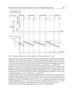
According to the architecture proposed and shown in Figure 3, a total of 1004 Twitter
comments were gathered from January 26, 2011 until March 29, 2011. An example of twitts
comments are shown in Table 1.
Then, a manual classification was performed on a subset of 200 comments, to label them into
positive, negative, or neutral categories, in order to use them as testing and training sets to
be input to the Support Vector Machine devised. The results of the classification process
performed over the entire data set are shown in Table 2.
Given the result in Table 2, the behavior of the demand must be expected to grow. How
much growing in the demand should be expected is matter of a business intelligence system.
These scattered signals gathered in the system we propose, must act jointly with systems at
every level in the logistics chain to prepare each company for the situation ahead. According
to our solution schema, this information should be passed through the highway capacity
framework to the SCOR supply chain model and plan accordingly. Action regarding
selection of transportation routes and modes as well as production, supply, and logistics
processes planning in the supply chain should take place after feedback information is

Supply Chain Management - New Perspectives

270
obtained. Long term planning must take place based on aggregated information, both from
structured and unstructured information.

Grapes growers /
vineyards

Wineries /
processin g
facilities
Irrigation
Technology
Gr ap e
harvesting &
filtration
equ
i
p
m
e
nt
Other
accessories and
equipment
Fert ilizer,
pesticides,
herbicides
Global
distribuition and
supply network
Barrels and
tanks
Bottles Caps & corks
PR &
A dvert isement
Labels Bot t ling

Fig. 5. Premium Chilean wine supply chain.

Date Comment Category
01/26/11 10:47 PM
Tabali Reserva Especial 2008 Syrah

neutral
02/02/11 10:52 PM
So Jr. wants to do study abroad in Chile next
year. My 1st question is "How much wine can
you bring back home?" Me loves Chilean wine.
positive
02/04/11 03:32 PM
Jeez, you could clean windows with these
personalized bottles of chemically-enhanced
Chilean wine.
negative
02/10/11 03:50 PM
Enjoying a Chilean wine this Valentine's Day?
Whether it's red, white, sparkling or still, we
want to hear about it!
positive
Table 1. Examples of twitts about "Chilean wine"

Neutral Positive Negative
Accuracy 19.64% 95.71% NA
Percentage 38% 60% 2%
Table 2. Performance measurements of sentiment classificator.
6. Conclusion
An integrated framework based on SCOR and CDMF by the U.S. Transportation Research

Board for modeling supply chains is proposed. The proposed framework is comprehensive
in terms of considering all the processes taking place in the supply chain for a given product
and at the same time assist by taking into account the transportation system capacity. We
also propose the operation of the supply chain model, obtained with the integrated

Information Gathering and Classification for Collaborative Logistics Decision Making

271
framework, should operate considering both structured data (available mostly in companies
or government agencies databases) and unstructured data (available from web sources such
as social networks). However, the enrichment that unstructured data provides to classical
decision making processes is important but does not eliminates the need for structured data.
Nevertheless, the amount of unstructured data available on the web is increasing by the
minute and its processing requires of powerful technologies of data processing and storage,
becoming available in a continuous basis. Thus, the processing of huge amounts of,
apparently, unrelated data produces rich information at low price, situation that has no
comparison to structured data (or that might be obtained at a very high price). The proposed
integrated framework and information retrieval assisting technology is scalable to supply
chains and applications in fields other than logistics.
8. Appendix








Fig. A1. Collaborative Decision-Making Framework Entry Level (SHRP 2, 2010)

Supply Chain Management - New Perspectives

272

Fig. A2. Collaborative Decision-Making Framework Practitioner Level (SHRP 2, 2010)
9. References
Bishop C. (2006). Pattern Recognition and Machine Learning. Springer.
Coelho, A. (2003), Presentation at an EADI workshop on Clusters and Global Value Chains in the
North and the Third World, organized at the Università del Piemonte Orientale,
Novara, Italy, October 30-31.
Corsten, H., 2001. Einführung in das Supply Chain Management. R. Oldenbourg Verlag,
München.
Cristianini, N. & Shawe-Taylor, J. (2000). Support Vector Machines and other kernel-based
learning methods, Cambridge University Press, 2000.
Duin R. P. W. & Pękalska E. (2006) Object Representation, Sample Size, and Data Set
Complexity, Data Complexity in Pattern Recognition, J. Lakhmi, W. Xindong (Ed.),
Springer London.
Fink E. (2001) Automatic evaluation and selection of problem-solving methods: Theory and
experiments, Journal of Experimental and Theoretical Artificial Intelligence 16(2) (2004),
pp. 73-105.
Holts, A., Riquelme, C. & Alfaro, R. (2010) Automated Text Binary Classification Using
Machine Learning Approach, Proceedings of the Chilean Society of Computer
Science Conference (SCCC), Antofagasta, November 2010, pp. 212-217.
Hvolby, H. & Trienekens, J. (2010). Challenges in business systems integration. Computers in
Industry, 61 (August 2010), pp. 808–812

Information Gathering and Classification for Collaborative Logistics Decision Making

273
Keikha M., Razavian N.Sh., Oroumchian F. & Razi H. S. (2008) Document representation

and quality of text: An analysis. In Survey of Text Mining II: Clustering, Classification,
and Retrieval, Springer-Verlag, London, pp. 135-168.
Lan M., Tan Ch. L., Su J. & Lu Y. (2009), Supervised and traditional term weighting methods
for automatic text categorization, IEEE Transactions on Pattern Analysis and Machine
Intelligence 31, 721-735.
Manning Ch. & Schütze H. (1999), Foundations of statistical natural language processing, The
MIT Press.
NSTPRSC. 2008. Transportation for Tomorrow. National Surface Transportation Policy and
Revenue Study Commission, Transportation Research Board. (2008). Available from

papers.htm
Pang B. & Lee L. (2008), Opinion Mining and Sentiment Analysis, Foundations and Trends in
Information Retrieval, v.2 n.1-2, pp. 1-135.
Qi X. & Davison B. D. (2009) Web page classification: features and algorithms, ACM
Computing Surveys, vol 41 N°2, Article 12.
Röder, A. & Tibken, B (2006). A methodology for modeling inter-company supply
chains and for evaluating a method of integrated product and process
documentation. European Journal of Operational Research, 169 (April 2005), pp.
1010–1029
Salton G. & Buckley Ch. (1988) Term-weighting approaches in automatic text retrieval,
Information Processing and Management: an International Journal 24, no. 5, pp. 513-
523.
Schönsleben, P., 2000. Integrales Logistikmanagement—Planung und Steuerung von
umfassenden Geschäftsprozessen. Springer-Verlag, Berlin.
Sebastiani F. (2002) Machine learning in automated text categorization, ACM Comput.
Surveys 34, no. 1, pp. 1-47.
SHRP 2, 2010. Performance Measurement Framework for Highway Capacity Decision-
Making, Strategic Highway Research Program 2, Transportation Research Board.
(2010). Available from
Sun A., Lim E. P. & Ng W. K. (2002) Web classification using support vector machine. In

Proceedings of the 4th International Workshop on Web Information and Data Management
(WIDM). ACM Press, New York, NY, pp. 96–99.
Supply Chain Council, 2010. Supply-Chain Operations Reference-model—Overview of SCOR
Version 10.0, Pittsburgh. Available from:
Trkman, P, McCormack K., Oliveira M. P. V. & Ladeira M. B., (2010) The Impact of Business
Analytics on Supply Chain Performance. Decision Support Systems, Vol. 49, No. 3,
pp. 318–327.
Tsoumakas G., Katakis I. & Vlahavas I. (2010), Mining multi-label data, Data Mining and
Knowledge Discovery Handbook, 2nd edition, O. Maimon, L. Rokach (Ed.),
Springer.
Vapnik, V. N. (1989). Statistical Learning Theory. Wiley-Interscience.

Supply Chain Management - New Perspectives

274
Visser, E. 2004. A Chilean wine cluster? Governance and upgrading in the phase of
internationalization. (September 2004). ECLAC/GTZ project on “Natural Resource
Based Strategies Development” (GER 99/128)
Williams, T.J. (1992). The Purdue Enterprise Reference Architecture, Instrument Society of
America, Research Triangle Park, USA, 1992.


Supply Chain Management - New Perspectives
276
materials. In general by-pass flows are admissible, e.g. from the source level to customers,
i.e. points of demand (Pods).


Fig. 1. A generic supply chain network
Supply chain management (SCM) is the integration of key business processes among a

network of interdependent suppliers, manufacturers, distribution centers, and retailers in
order to improve the flow of goods, service, and information from original suppliers to final
customers, with the objective of reducing system-wide costs while maintaining required
service levels (Simchi-Levi et al. 2000).
Stadtler (2005) presents a framework for the classification of SCM and advanced planning
issues and targets: there are several commercial software packages available for advanced
planning, the so-called advanced planning systems (APS), incorporating models and
solution algorithms and tools widely discussed by the literature. In particular, Su and Yang
(2010) discuss the importance of enterprise resource planning (ERP) systems for improving
overall SC performance. ERP systems are essential enablers of SCM competences.
Nevertheless there are not yet valuable integrated tools as supporting decisions makers for
planning strategic, tactical and operational issues and activities of a wide and complex
logistic network. In particular, ERP systems and APSs do not support decision making on
the whole system (logistic network) optimization and design. The great complexity of such a
problem forces the managers to accept local optima as sub optimizations renouncing to
identify the best configuration of the whole network. The so-called best configuration
usually corresponds to an admissible solution of minimum logistic cost and/or maximizes
customer’s service levels.
Planning a SC network involves making decisions to cope with long-term strategic
planning, medium-term tactical planning and short-term operational planning as
summarized in Figure 2.
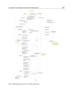
Figure 3 reports main decisions for the strategic planning (e.g. supplier selection, production
facilities location), the tactical planning (master production planning, DCs assignment,
storage capacity determination) and the short time operational planning and scheduling

A Supporting Decision Tool for the Integrated Planning of a Logistic Network
277
(scheduling, multi-facility MRP, vehicle routing) classified in terms of decision typology:
purchase & production decisions, distribution decisions and supply decisions (Manzini and
Bindi, 2009).

Fig. 2. Classification of planning decisions


Fig. 3. Issues and decisions (Manzini and Bindi, 2009)
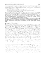
2.1 Strategic planning
The strategic level deals with decisions that have a long-lasting effect on a company (Simchi-
Levi et al. 2004) and supports the design and configuration of a logistic network. The terms
“network design” and “SC network design” are usually synonymous of strategic SC
planning. Melo et al. (2009) classify the literature on strategic planning in accordance with
some typical SC decisions: capacity decisions, inventory decisions, procurement decisions,

Supply Chain Management - New Perspectives
278
production decisions, routing decisions, and the choice of transportation modes. Additional
features of facility locations models in SCM environment are: financial aspects (e.g.
international factors, incentives offered by governments, budget constraints for opening and
closing facilities), risk management (uncertainty in customer demands and costs, reliability
issues, risk pooling in inventory management), and other aspects, e.g. relocation, bill of
material (BOM) integration, and multi period factors. To avoid sub-optimization, these
decisions should be regarded in an integrated perspective (Melo et al. 2009).
As a consequence, the strategic planning usually deals with long-term decisions, single period
modelling, and the so-called location allocation problem (LAP) (Manzini and Bindi, 2009).
The strategic planning can be considered as the design of a “static network”: the aim is the
determination of the best configuration, i.e. the architecture, of the logistic system.
2.2 Tactical planning
The tactical planning deals with medium-term and short-term decisions by a multi-period
modelling. This planning activity defines the best configuration of the multi-echelon
inventory distribution fulfilment system. It generates also the list of deliveries/shipments

between suppliers and customers at different stages of the distribution system. As a
consequence the aim of the tactical planning is the determination of the best configuration
and management of the fulfilment system. The tactical planning is similar to a multi-echelon
and time-dependent capacity constraint material requirement planning (MRP) combined to
a distribution requirement planning (DRP). This planning is multi-product (i.e. multi-
commodity), multi-period and the duration of the planning horizon of time is generally a
few months. Different transportation modes are available. Storage, handling and production
capacities are modelled for each distribution/production center.
2.3 Operational planning
As a result of the application of a multi-period tactical planning to a distribution network,
the logistic manager needs to daily supply products to a large set of customers/consumers,
the so-called points of demand (Pods), by the adoption of a set of different transportation
modes. The operational planning of a SC network deals with the short-term scheduling of
vehicle missions & trips necessary to supply products to the demand points, in presence (or
in absence) of the groupage strategy. This strategy consists in defining groups of Pods that
can be visited by a vehicle in a single trip. Consequently, adopting the groupage strategy the
customers/Pods are grouped in disjunctive pools and a single vehicle serves the members of
each group simultaneously in a multi-stop (multi-visit) trip (route/mission). This is the
well-known vehicle routing problem (VRP), which is a non-deterministic polynomial-time
hard (NP-hard) combinatorial optimization and nonlinear programming problem seeking to
service a number of customers with a fleet of vehicles (Baldacci and Mingozzi 2009, Dantzig
and Ramser 1959). In particular CVRP is the so-called capacitated VRP, where a fixed fleet of
delivery vehicles of uniform capacity must serve known customer demands from a common
depot, e.g. a distribution center CD, at minimum transit cost (Güneri 2007).
In SC planning, given a point in time t, e.g. a day, and a defined depot (e.g. a production
plant, a central distribution center CDC, a regional distribution center RDC), there are many
Pods assigned to that facility as the result of a tactical planning: their demand values are
allocated to that facility in t. For example in presence of a 3-stage and four levels SC made
of production Plants (level 1), CDCs (level 2), RDCs (level 3), customer Pods (level 4), it can

A Supporting Decision Tool for the Integrated Planning of a Logistic Network
279
be necessary to define the daily scheduling of deliveries from the central DCs to the regional
DCs, and the daily scheduling from the RDCs to the customers in presence of fractionable
and/or non fractionable (single-sourcing hypothesis) demand of products, and adopting
and/or non adopting the groupage strategy.
The daily SC planning is a very complex problem and consists in defining the best groups of
customers and the best geographical routings minimizing the global logistic costs in
accordance to different kinds of constraints, e.g. time windows, load capacities, pickup and
delivery sequencing, set-up, etc. Literature presents several models and methods to help the
manager to find good solutions; but they are generally very complex and not effective given
a real instance/application of the transportation problem characterized by a realistic
dimension, e.g. hundreds of Pods and many depots.
3. A framework for an integrated planning
Figure 4 presents the conceptual framework of the proposed integrated planning process.
The proposed automatic tool LD-LogOptimizer has adopted this framework. It is a multi-
step supporting decisions framework for strategic, tactical and operational planning
activities. This is the basis for the development of an automatic tool, named LD-
LogOptimizer. LD-LogOptimizer is illustrated in this chapter and has been applied to a
significant case study as discussed in last sections of this chapter. This tool deals with many
input data and generates a lot of results and system performance as discussed below.


Fig. 4. Framework for an integrated planning of a distribution network
Figure 5 presents the input data to be collected for the implementation of the approach
briefly illustrated in Figure 4. For the generic Pod: geographical location and demand
quantity for each product and each point in time t, e.g. daily demand. For the generic RDC
and CDC: location, fixed operating cost, variable operating (inventory and handling) costs,
maximum admissible capacities (storage and handling). For the generic production plant:
location, fixed operating cost, variable unit costs (also including the production unit cost),

maximum admissible capacities (also including the production capacity), etc.

Supply Chain Management - New Perspectives
280

Fig. 5. Input data for the implementation, logic scheme
3.1 Strategic planning in LD-LogOptimizer
Figure 6 illustrates the strategic planning as modelled and implemented by the proposed
automatic tool LD-LogOptimizer. In particular, given previously illustrated input data, a 3-
stage (4-levels) single-period multi-product mixed integer linear programming (MILP)
model for the location allocation problem (LAP) is defined. Euclidean distances are
generally adopted to model the distances between two locations, e.g. a source and a RDC. A
set of input data on variable and fixed costs and vehicles’ settings has to be introduced
because different transportation modes are available.
The model can be solved as-is (see "strategic model 3S" in Figure 6) or reducing the number
of levels from four to three (i.e. the number of stages to two) by the generation of two
distinct sub-problems: the assignment of Pods demand to RDCs by the execution of a
heuristic rule and the assignment of materials flows to the higher levels of the network
(from RDCs to the sources passing from the CDCs). The in-depth illustration of the
heuristics is not the aim of this chapter. The simplification introduced by the heuristic
approach to problem solving significantly reduces the computational complexity of the
decision problem: the as-is "strategic model 3S" is substituted by the so-called heuristic rule
at the first stage combined with the "strategic model 2S" at the second and third stages. The
as-is problem modelling is for the optimal solution of the LAP; the simplified reduces the
computational time but accept feasible solution very closed to the unknown optimal one.
The strategic planning as reported in Figure 6 generates a large number of output results.
3.2 Tactical planning in LD-LogOptimizer
The tactical planning implemented by LD-LogOptimizer is illustrated in Figure 7. The
dynamic multi-period, multi-product, multi-transportation mode, 3-stage LAP can be solved
as a result of the application of the so-called "pre-setting" process (see Figure 7), i.e. by the

activation of facilities and/or flows and/or transportation modes adopted at the strategic
decisional step, or as an optimization problem without assuming any hypothesis/decision
generated at the previous step. In absence of pre-setting the model is called "tactical model
3S" (see Figure 7). Examples of output data, mainly time based, for the tactical planning are:
inventory levels at production/distribution facilities, material flows, picking/delivery lists
of products at the generic Pod for a point in time t, transportation mode adopted for a
specific product from a supplier level to a point of demand level in t, costs, etc.
3.3 Operational planning in LD-LogOptimizer
Figure 8 illustrates the adopted operational planning for a 3-stage, multi-period, multi-
product, multi- (transportation) -mode. It is a cluster-first and route-second procedure based


A Supporting Decision Tool for the Integrated Planning of a Logistic Network
281

Fig. 6. Strategic planning, LD-LogOptimizer

Supply Chain Management - New Perspectives
282

Fig. 7. Tactical planning, LD-LogOptimizer

A Supporting Decision Tool for the Integrated Planning of a Logistic Network
283


Fig. 8. Operational Planning, LD-LogOptimizer
on the introduction of original similarity indices for clustering of demand points (e.g. Pods
at the first stage RDCs-Pods or RDCs at the second stage CDCs-RDCs) and
sequencing/routing of visits (e.g. Pods) within each cluster of demand points assigned to a

supplier (e.g. an RDC). Examples of output data generated by the tool are: configuration of
clusters, vehicle loading and saturation, vehicle routing, routes, costs, distances, etc.
Figure 9 shows the conceptual framework adopted by LD-LogOptimizer as the integration
of strategic, tactical and operational planning activities.

Supply Chain Management - New Perspectives
284

Fig. 9. LD-LogOptimizer tool for the integrated planning
4. A case study
This case study refers to a 3-stage US distribution system operating in USA and made of:
 3 production plants located in Sacramento (California), Philadelphia (Pennsylvania) and
Topeka (Kansans);
 3 CDCs located in Baltimore (Maryland), Kansas City (Missouri) and Reno (Nevada);
 12 RDCs whose location, capacities and costs are reported in Table 1;
 120 Pods all located in USA;
 the number of time units for the planning period is 20 corresponding to days (20 days
are about one month);
 3 transportation modes are available: truck, train and plane.

A Supporting Decision Tool for the Integrated Planning of a Logistic Network
285


Table 1. Regional distribution centers - RDC
4.1 Strategic planning, case study
Figure 10 shows the main form of the strategic planning in LD-LogOptimizer. It is made of
different sections for input and output data. A quick report guides the user to the full
comprehension of the tool activities. Figure 11 presents the input data including the
geographical map. In particular, on the map yellow flags represent the production plants

(sources), white flags the RDCs, light blue flags the CDCs, green flags the Pods.
Figure 12 shows the results of the application of the strategic planning: the activated nodes
of the network and the activated material flows are visible. For example, RDC1 and RDC6
are closed at the third stage of the system; Pod98 is supplied by RDC3 that supplies also
other points of demand, e.g. Pod99, Pod101, Pod106. The total logistic cost and different
contributions are reported in the quick report.
6 of 12 available RDCs are closed; 1 of 3 available CDCs is activated (open); 1 of 3 available
plants is open. Closed plants are represented in black colour, in blue closed CDCs and in red
closed RDCs. Figure 12 show also the flows of material for a specific product at the first stage.
Figure 13 presents the results of the strategic planning showing also the flows at the third
stage (RDCs-Pods). Similarly Figure 14 shows the flows activated by product P2.
Figure 15 reports the graph of the distribution of costs within the system as the result of the
strategic planning in LD-LogOptimizer: about 21% of the total cost is due to transportation
activities; about 34% to fixed costs (e.g. to open/activate facilities as CDCs and RDCs); about
45% of the total cost is variable (e.g. handling cost).
Table 2 presents the obtained results in terms of KPI. The activated facilities are: 6 of 12
RDCs, 1 of 3 CDCs, 1 of 3 production plants. The total cost refers to the whole planning
period of one year. It is a very expensive cost because it includes all fixed cost contributions
necessary to build the network, i.e. to open/active logistic facilities, and to move materials
from suppliers to demand points.
4.2 Tactical planning, case study
Tactical planning is a time-dependent planning. Consequently, for each product and the
generic point in time t a set of facilities and materials flows are activated in order to ship
products from sources (production plants) to Pods passing through CDC and RDC facilities,
in accordance with capacity constraints, lead time, variable and fixed unit costs, etc.
Id Address Zip City Country
Activation
cost[€]
Handling
variable

cost
[€/load]
Handling
capacity
[load]
Storage
variable
cost
[€/load]
Storage
capacity
[load]
RDC1 425TolandSt 94124 SanFrancisco,California USA 11129000 0.09 1950000 0.05 115000
RDC2 2768WinonaAve 91504 Burbank,California USA 11129000 0.09 1950000 0.05 115000
RDC3 768TaylorStationRd 43230 Columbus,Ohio USA 11129000 0.09 1950000 0.05 115000
RDC4 1890ElmTreeDr 37210 Nashville,Tennessee USA 11129000 0.09 1950000 0.05 115000
RDC5 393TellurideSt 80011 Aurora,Colorado USA 11129000 0.09 1950000 0.05 115000
RDC6 509CarrollSt 11215 Brooklyn,NewYork USA 11129000 0.09 1950000 0.05 115000
RDC7 7 211SLockwoodAve 60638 Chicago,Illinois USA 11129000 0.09 1950000 0.05 115000
RDC8 3640AtlantaIndustrialDrNW 30331 Atlanta,Georgia USA 11129000 0.09 1950000 0.05 115000
RDC9 618WWestSt 21230 Baltimore,Maryland USA 11129000 0.09 1950000 0.05 115000
RDC10 3915SWMoodyA ve 97239 Portland,Oregon USA 11129000 0.09 1950000 0.05 115000
RDC11 2412CommercialSt 72206 LittleRock,Arkansas USA 11129000 0.09 1950000 0.05 115000
RDC12 5518Export
Blvd 31408 Savannah,Georgia USA 11129000 0.09 1950000 0.05 115000

Supply Chain Management - New Perspectives
286

Fig. 10. Strategic planning, LD-LogOptimizer, main form

Fig. 11. Input data for the strategic planning

A Supporting Decision Tool for the Integrated Planning of a Logistic Network
287

Fig. 12. Results, strategic planning


Fig. 13. Product 1, strategic planning. Flows at the first stage.

Supply Chain Management - New Perspectives
288

Fig. 14. Product 2, materials flows. Strategic planning.


Fig. 15. Strategic planning, network cost.
Figure 16 presents the result of the execution of LD-LogOptimizer on the case study object
of the analysis and for the tactical planning. In particular, results in figure refer to the
product named P1. The list of deliveries for the active RDCs to the Pods in the point in time
T1 is also reported: this is the input for the operational planning illustrated in next
subsection. Flows of product P1 between active facilities in T1 are shown.
Figure 17 shows the material flows of another product, P2, for the period of time T1.

A Supporting Decision Tool for the Integrated Planning of a Logistic Network
289

Table 2. Strategic planning, KPI

Fig. 16. Tactical planning, case study
KPIStrategicPlanning Value
Pointsofdemand 120
RDC 12
CDC 3
Plants 3
RDCactivated 6
CDCactivated 1
Plantsactivated 1
TOTALCOST[€] 479196000
RDCcost[€] 98235760
CDCcost[€] 37760600
Plantcost[€] 242053800
3°stagetrasportationcost[€] 42149040
2°stagetrasportationcost[€] 53662470
1°stagetrasportationcost[€] 5334346
Averagen°ofpointsof demandservedbyaregionaldistributioncenter 10.24
Averagen°ofregional
distributioncentersthatserveapointof demand 0.51
Averagen°ofregionaldistributioncentersservedbyacentraldistributioncenter 5.97
Averagen°ofcentraldistributioncentersthatservearegionaldistributioncenter 0.99
Averagen°ofcentraldistributioncentersservedbyaplant 1
Averagen°ofplantsthatserveacentraldistribution center 1
Average
3°stagedistance[km] 835.03
Average2°stagedistance[km] 1175.36
Average1°stagedistance[km] 103.78

Supply Chain Management - New Perspectives
290

Fig. 17. Tactical planning (P2 in T1)
Table 3 presents the obtained results in terms of KPI for the tactical planning. In particular,
the expected costs significantly differ from the strategic planning costs because they refer to
the planning period made of 20 units of time. The activated facilities are: 6 of 12 RDCs, 1 of 3
CDCs, 1 of 3 production plants. An RDC serves about 10-11 Pods.


Table 3. Tactical planning, KPI
KPITac tialPlanning Value
Pointsofdemand 120
RDC 12
CDC 3
Plants 3
RDCactivated 6
CDCactivated 1
Plantsactivated 1
TOTALCOST[€] 19584910
RDCcost[€] 3542925
CDCcost[€] 1197645
Plantcost[€] 9232994
3°stagetrasportationcost[€] 3171216
2°stagetrasportationcost[€] 2227638
1°stagetrasportationcost[€] 212496
Averag en°ofpoi ntsofdeman dservedbyaregionaldistributioncenter 10.26
Averag en°ofregional
distributioncentersthatserveapointofdemand 0.51
Averag en°ofregionaldistributioncentersservedbyacentraldistribution center 5.96

Averag en°ofcentraldistribution centersthatservearegionaldistributioncenter 0.99
Averag en°ofcentraldistribution centersservedbyaplan t 1
Averag en°ofplantsthatserveacentraldistributioncenter 1
Averag e
3°stagedistance[km] 834.07
Averag e2°stagedistance[km] 1174.56
Averag e1°stagedistance[km] 103.78

A Supporting Decision Tool for the Integrated Planning of a Logistic Network
291
4.3 Operational planning, case study
The operational planning can be applied to plan and schedule the vehicle routing at the each
stage of the network and in particular from RDCs to Pods and from CDCs to RDCs. The first
of this stage usually involves trucks as transportation modes; while CDCs-RDCs shipments
can be executed also adopting one of the other available modes (e.g plane and train).
Figure 18 presents a result obtained by the execution of the operational planning on the case
study. A list of clusters is reported and for each cluster it is possible to generate the optimal
route as the minimum Hamiltonian circuit visiting all the members grouped in a cluster.
The route ID 173 is shown. It is made of the following sequence of visits: RDC4, Pod106,
Pod110, Pod111, Pod109, Pod108, Pod107, RDC4. Another detailed route is exemplified in
Figure 19. The groupage strategy can reduces the cost of travelling of about 55% if compared
with direct delivery, i.e. direct shipment from a generic supplier to a point of demand.
Figure 20 exemplifies another route (named ID 109) departing from Chicago and generated
by the operational planning.

Fig. 18. Operational planning, route ID 173