Vibration Analysis and Control New Trends and Developments Part 4 pdf
Bạn đang xem bản rút gọn của tài liệu. Xem và tải ngay bản đầy đủ của tài liệu tại đây (3.54 MB, 25 trang )
Seismic Response Reduction of Eccentric Structures Using Liquid Dampers
65
2
2
0
2
22
2
14
()
14
g
l
gg
S
ω
β
ω
ω
ωω
β
ωω
⎛⎞
+⎜⎟
⎜⎟
⎝⎠
Φ=
⎡⎤
⎛⎞ ⎛⎞
⎢⎥
−⎜ ⎟ + ⎜ ⎟
⎜⎟ ⎜⎟
⎢⎥
⎝⎠ ⎝⎠
⎣⎦
(33)
The parameters of this function are: 5
g
ω
π
=
, 0.5
β
=
,
0
0.01S = .
As mentioned before, two TLCDs and one CTLCD are installed at the top of the building.
The objective of the study is to design the optimum parameters of these dampers that would
maximize the performance function stated earlier. The possible ranges for the design
parameters are fixed as follows:
1.
Mass ratio, μ: The mass ratio is defined as the ratio of the damper mass to the total
building mass. It is assumed that each damper ratio can vary in the range of 0.1 percent
to 1 percent of the building mass. Thus the maximum mass of the damper system
consisting of three dampers could be as high as 3 percent of the building mass.
2.
Frequency tuning ratio, f: The frequency ratio for each damper is defined as the ratio its
own natural frequency to the fundamental frequency of the building structure. Here it
is assumed that this ratio could vary between 0-1.5.
3.
Damping ratio, d: This is a ratio of the damping coefficient to its critical value. It is
assumed that this ratio can vary in the range of 0-10 percent.
4.
Damper positions from the mass center, lx in x axis and ly: in y axis: It is assumed that lx
can vary between –8 and 5 meters and ly can vary between –4 and 3 meters
The optimization process starts with a population of these individuals. For the problem at
hand, 30 individuals were selected to form the population. The probability of crossover and
mutation are 0.95 and 0.05, respectively. The process of iteration is determined to be 300 steps.
The final optimum parameters for the two optimum design criteria are given in Table 2.
Performance Criteria i (f1=0.47769)
TLCD in x direction TLCD in y direction CTLCD
μ
0.008519 0.0095655 0.0014362
f
r
1.2334 0.96607 1.1137
d
r
0.053803 0.061988 0.052886
l
x
-7.38 0.45567 —
l
y
-6.479 -2.2431 —
Table 2. The optimal parameters of liquid dampers
3.4 Seismic analysis in time domain
The parameters of liquid dampers on the 8-story building structure have been optimized in
the previous section and the results are listed in the Table 2. The control results of liquid
dampers on the building are analyzed in time domains in this section. The El Centro, Tianjin
and Qian’an earthquake records are selected to input to the structure as excitations, which
represent different site conditions.
The structural response without liquid dampers subjected to earthquake in x, y and θ
directions are expressed with x
0
, y
0
and θ
0
, respectively. Also, the response with liquid
Vibration Analysis and Control – New Trends and Developments
66
dampers subjected to earthquake in x, y and θ directions are expressed with x, y and θ,
respectively. The response reduction ratio of the structure is defined as
0
0
100%
xx
J
x
−
=×
(34)
The maximum displacements of the structure and response reduction ratios are computed
for three earthquake records and the results listed from Table 3 to Table 5. It can be seen
Story
Number
x
0
(cm)
x
(cm)
J
(%)
y
0
(cm)
y
(cm)
J
(%)
θ
0
(10
-4
Rad)
θ
(10
-4
Rad)
J
(%)
1 0.57 0.53 6.14 1.18 0.99 15.94 1.71 1.56 8.77
2 1.11 1.03 7.24 2.28 1.94 15.12 3.30 3.04 7.88
3 1.77 1.58 10.71 3.43 2.96 13.73 5.02 4.61 8.17
4 2.38 2.04 14.20 4.30 3.76 12.59 6.42 5.87 8.57
5 2.98 2.54 15.01 4.95 4.39 11.34 7.62 6.90 9.45
6 3.48 3.03 12.77 5.64 4.69 16.76 8.50 7.46 12.24
7 4.03 3.67 8.86 6.58 4.89 25.64 10.05 8.63 14.13
8 4.37 4.06 7.00 7.10 5.47 22.98 10.96 9.63 12.14
Table 3. Maximum displacements of the structure (El Centro)
Story
Number
x
0
(cm)
x
(cm)
J
(%)
y
0
(cm)
y
(cm)
J
(%)
θ
0
(10
-4
Rad)
θ
(10
-4
Rad)
J
(%)
1 2.49 1.85 25.64 2.10 1.83 12.57 4.67 4.22 9.64
2 4.91 3.66 25.49 4.05 3.52 13.03 9.14 8.25 9.74
3 7.71 5.78 25.06 6.30 5.48 13.12 14.21 12.73 10.42
4 10.26 7.69 24.98 8.36 7.23 13.59 18.83 16.75 11.05
5 12.77 9.58 24.97 10.36 8.90 14.08 23.21 20.60 11.25
6 14.79 11.09 24.97 11.98 10.27 14.25 26.55 23.56 11.26
7 16.88 12.66 24.96 14.10 12.13 13.91 30.45 27.05 11.17
8 17.98 13.51 24.89 15.22 13.41 11.90 32.44 29.02 10.54
Table 4. Maximum displacements of the structure (Tianjin)
Story
Number
x
0
(cm)
x
(cm)
J
(%)
y
0
(cm)
y
(cm)
J
(%)
θ
0
(10
-4
Rad)
θ
(10
-4
Rad)
J
(%)
1 0.11 0.10 6.91 0.10 0.091 6.93 0.132 0.12 4.10
2 0.19 0.17 6.57 0.19 0.16 16.00 0.25 0.24 1.25
3 0.23 0.21 6.66 0.28 0.22 24.60 0.39 0.38 2.82
4 0.24 0.21 11.48 0.38 0.28 25.86 0.51 0.50 1.45
5 0.29 0.22 23.54 0.48 0.36 24.89 0.63 0.61 1.40
6 0.34 0.26 24.76 0.56 0.43 23.54 0.72 0.70 2.20
7 0.39 0.34 14.17 0.70 0.54 21.70 0.83 0.79 4.45
8 0.43 0.39 8.15 0.77 0.62 19.47 0.93 0.87 5.60
Table 5. Maximum displacements of the structure (Qian’an)
Seismic Response Reduction of Eccentric Structures Using Liquid Dampers
67
Fig. 17. Time history of the displacement on the x direction of top floor (El Centro)
Fig. 18. Time history of the displacement on the
y
direction of top floor (El Centro)
Fig. 19. Time history of the torsional displacement of top floor (El Centro)
Vibration Analysis and Control – New Trends and Developments
68
from the tables that the responses of the structure in each degree of freedom are reduced
with the installation of liquid dampers. However, the reduction ratios are different for the
different earthquake records.
The displacement time history curves of the top story are shown from Fig. 6 to Fig. 8 and
acceleration time history curves in Fig. 17 to Fig. 19 for El Centro earthquake. It can be seen
from these figures that the structural response are reduced in the whole time history.
4. Conclusion
From the theoretical analysis and seismic disasters, it can be concluded that the seismic
response is not only in translational direction, but also in torsional direction. The torsional
components can aggravate the destroy of structures especially for the eccentric structures.
Hence, the control problem of eccentric structures under earthquakes is very important. This
paper focus on the seismic response control of eccentric structures using tuned liquid
dampers. The control performance of Circular Tuned Liquid Column Dampers (CTLCD) to
torsional response of offshore platform structure excited by ground motions is investigated.
Based on the equation of motion for the CTLCD-structure system, the optimal control
parameters of CTLCD are given through some derivations supposing the ground motion is
stochastic process. The influence of systematic parameters on the equivalent damping ratio
of the structures is analyzed with purely torsional vibration and translational-torsional
coupled vibration, respectively. The results show that Circular Tuned Liquid Column
Dampers (CTLCD) is an effective torsional response control device. An 8-story eccentric
steel building, with two TLCDs on the orthogonal direction and one CTLCD on the mass
center of the top story, is analyzed. The optimal parameters of liquid dampers are optimized
by Genetic Algorithm. The structural response with and without liquid dampers under bi-
directional earthquakes are calculated. The results show that the torsionally coupled
response of structures can be effectively suppressed by liquid dampers with optimal
parameters.
5. Acknowledgment
This work was jointly supported by Natural Science Foundation of China (no. 50708016 and
90815026), Special Project of China Earthquake Administration (no. 200808074) and the 111
Project (no. B08014).
6. References
Bugeja, N.; Thambiratnam, D.P. & Brameld G.H. (1999). The Influence of Stiffness and
Strength Eccentricities on the Inelastic Earthquake Response of Asymmetric
Structures, Engineering Structures, Vol. 21,No.9, pp.856–863
Chang, C. C. & Hsu, C. T.(1998). Control Performance of Liquid Column Vibration
Absorbers. Engineering Structures. Vol.20, No.7, pp.580-586
Chang, C. C.(1999). Mass Dampers and Their Optimal Design for Building Vibration
Control. Engineering Structures, Vol.21, No.5, pp.454-463
Seismic Response Reduction of Eccentric Structures Using Liquid Dampers
69
Fujina, Y. & Sun, L. M.(1993). Vibration Control by Multiple Tuned Liquid
Dampers(MTLDs). J. of Structural Engineering, ASCE, Vol.119, No.12,
pp.3482-3502
Gao H. & Kwok K. C. S.(1997). Optimization of Tuned Liquid Column Dampers. Engineering
Structures, Vol.19, No.6, pp. 476-486
Gao, H.; Kwok, K. S. C. & Samali B.(1999). Characteristics Of Multiple Tuned Liquid
Column Dampers In Suppressing Structural Vibration. Engineering Structures,
Vol.21, No.4, pp.316-331
Hitchcock, P. A.; Kwok, K. C. S. & Watkins R. D. (1997). Characteristics Of Liquid Column
Vibration Absorbers (LCVA)-I. Engineering Structures, Vol.19, No.2, pp.126-134
Hitchcock, P. A.; Kwok, K. C. S. & Watkins R. D. (1997). Characteristics Of Liquid Column
Vibration Absorbers (LCVA)-II. Engineering Structures, Vol.19, No.2,
pp.135-144
Hochrainer, M. J.; Adam, C. & Ziegler, F. (2000). Application of Tuned Liquid Column
Dampers for Passive Structural Control, Proc. of 7th International Congress on Sound
and Vibration (ICSV 7), Garmisch-Partenkirchen, Germany, pp.3107-3114
Huo, L.S. & Li H.N. (2001). Parameter Study of TLCD Control System Excited by Multi-
Dimensional Ground Motions. Earthquake Engineering and Engineering Vibration,
Vol.21, No.4, pp.147-153
Jiang, Y. C. & Tang, J. X. (2001). Torsional Response of the Offshore Platform with TMD,
China Ocean Engineering, Vol.15, No.2, pp.309-314
Kareem, A. & Kline, S.(1995). Performance Of Multiple Mass Dampers Under Random
Loading. J. of Structural Engineering, ASCE, Vol.121, No.2, pp.348-361
Kim, H. (2002). Wavelet-based adaptive control of structures under seismic and wind loads.
Notre Dame: The Ohio State University
Li, H.N. & Wang, S.Y. (1992). Torsionally Coupled Stochastic Response Analysis of Irregular
Buildings Excited by Multiple Dimensional Ground Motions. Journal of Building
Structures, Vol.13, No.6, pp.12-20
Liang, S.G. (1996).Experiment Study of Torsionally Structural Vibration Control Using
Circular Tuned Liquid Column Dampers, Special Structures, Vol.13, No.3,
pp. 33-35
Qu, W. L.; Li, Z. Y. & Li, G. Q. (1993). Experimental Study on U Type Water Tank for Tall
Buildings and High-Rise Structures, China Journal of Building Structures, Vol.14,
No.5, pp.37-43
Sakai, F.; Takaeda, S. & Tamake, T. (1989). Tuned Liquid Column Damper — New Type
Device For Suppression Of Building Vibrations. Proc. Int. Conf. On High-rise
Buildings, Nanjing, China, pp.926-931
Wang, Z. M. (1997). Vibration Control of Towering Structures, Shanghai: Press of Tongji
University.
Yan, S. & Li H. N.(1999). Performance of Vibration Control for U Type Water Tank with
Variable Cross Section. Earthquake Engineering and Engineering Vibration, Vol.19,
No.1, pp.197-201
Vibration Analysis and Control – New Trends and Developments
70
Yan, S.; Li, H. N. & Lin, G. (1998). Studies on Control Parameters of Adjustable Tuned
Liquid Column Damper, Earthquake Engineering and Engineering Vibration, Vol18,
No.4, pp. 96-101
4
Active Control of Human-Induced Vibrations
Using a Proof-Mass Actuator
Iván M. Díaz
Universidad de Castilla-La Mancha
Spain
1. Introduction
Advances in structural technologies, including construction materials and design
technologies, have enabled the design of light and slender structures, which have
increased susceptibility to human-induced vibration. This is compounded by the trend
toward open-plan structures with fewer non-structural elements, which have less inherent
damping. Examples of notable vibrations under human-induced excitations have been
reported in floors, footbridges and grandstands, amongst other structures (Bachmann,
1992; Bachmann, 2002; Hanagan et al., 2003a). Such vibrations can cause a serviceability
problem in terms of disturbing the users, but they rarely affect the fatigue behaviour or
safety of structures.
Solutions to overcome human-induced vibration serviceability problems might be: (i)
designing in order to avoid natural frequencies into the habitual pacing rate of walking,
running or dancing, (ii) stiffening the structure in the appropriate direction resulting in
significant design modifications, (iii) increasing the weight of the structure to reduce the
human influence being also necessary a proportional increase of stiffness and (iv) increasing
the damping of the structure by adding vibration absorber devices. The addition of these
devices is usually the easiest way of improving the vibration performance. Traditionally,
passive vibration absorbers, such as tuned mass dampers (TMDs) (Setareh & Hanson, 1992;
Caetano et al., 2010), tuned liquid dampers (Reiterer & Ziegler, 2006) or visco-elastic
dampers, etc., have been employed. However, the performance of passive devices is often of
limited effectiveness if they have to deal with small vibration amplitude (such as those
produced by human loading) or if vibration reduction over several vibration modes is
required since they have to be tuned to a single mode. Semi-active devices, such semi-active
TMDs, have been found to be more robust in case of detuning due to structural changes, but
they exhibit only slightly improved performance over passive TMDs and they still have the
fundamental problem that they are tuned to a single problematic mode (Setareh, 2002;
Occhiuzzi et al., 2008). In these cases, an active vibration control (AVC) system might be
more effective and then, an alternative to traditional passive devices (Hanagan et al., 2003b).
A state-of-the-art review of technologies (passive, semi-active and active) for mitigation of
human-induced vibration can be found in (Nyawako & Reynolds, 2007). Furthermore,
techniques to cancel floor vibrations (especially passive and semi-active techniques) are
reviewed in (Ebrahimpour & Sack, 2005) and the usual adopted solutions to cancel
footbridge vibrations can be found in (FIB, 2005).
Vibration Analysis and Control – New Trends and Developments
72
An AVC system based on direct velocity feedback control (DVFC) with saturation has
been studied analytically and implemented experimentally for the control of human-
induced vibrations via an active mass damper (AMD) (also known as inertial actuator or
proof-mass actuator) on a floor structure (Hanagan & Murray, 1997) and on a footbridge
(Moutinho et al., 2010). This actuator generates inertial forces in the structure without
need for a fixed reference. The velocity output, which is obtained by an integrator circuit
applied to the measured acceleration response, is multiplied by a constant gain and feeds
back to a collocated force actuator. The term collocated means that the actuator and sensor
are located physically at the same point on the structure. The merits of this method are its
robustness to spillover effects due to high-order unmodelled dynamics and that it is
unconditionally stable in the absence of actuator and sensor (integrator circuit) dynamics
(Balas, 1979). Nonetheless, when such dynamics are considered, the stability for high
gains is no longer guaranteed and the system can exhibit limit cycle behaviour, which is
not desirable since it could result in dramatic effects on the system performance and its
components (Díaz & Reynolds, 2010a). Then, DVFC with saturation is not such a desirable
solution. Generally, the actuator and sensor dynamics influence the system dynamics and
have to be considered in the design process of the AVC system. If the interaction between
sensor/actuator and structure dynamics is not taken into account, the AVC system might
exhibit poor stability margins, be sensitive to parameter uncertainties and be ineffective.
A control strategy based on a phase-lag compensator applied to the structure acceleration
(Díaz & Reynolds, 2010b), which is usually the actual magnitude measured, can alleviated
such problems. This compensator accounts for the interaction between the structure and
the actuator and sensor dynamics in such a way that the closed-loop system shows
desirable properties. Such properties are high damping for the fundamental vibration
mode of the structure and high stability margins. Both properties lead to a closed-loop
system robust with respect to stability and performance (Preumont, 1997). This control
law is completed by: (i) a high-pass filter, applied to the output of the phase-lag
compensator, designed to avoid actuator stroke saturation due to low-frequency
components and (ii) a saturation nonlinearity applied to the control signal to avoid
actuator force overloading at any frequency. This methodology will be referred as to
compensated acceleration feedback control (CAFC) from this point onwards.
This chapter presents the practical implementation of an AMD to cancel excessive vertical
vibrations on an in-service office floor and on an in-service footbridge. The AMD consists of
a commercial electrodynamic inertial actuator controlled via CAFC. The remainder of this
chapter is organised as follows. The general control strategy together with the structure and
actuator dynamic model are described in Section 2. The control design procedure is
described in Section 3. Section 4 deals with the experimental implementation of the AVC
system on an in-service open-plan office floor whereas Section 5 deals with the
implementation on an in-service footbridge. Both sections contain the system dynamic
models, the design of CAFC and results to assess the design. Finally, some conclusions are
given in Section 6.
2. Control strategy and system dynamics
The main components of the general control strategy adopted in this work are shown in Fig.
1. The output of the system is the structural acceleration since this is usually the most
convenient quantity to measure. Because it is rarely possible to measure the system state
Active Control of Human-Induced Vibrations Using a Proof-Mass Actuator
73
and due to simplicity reasons, direct output measurement feedback control might be
preferable rather than state-space feedback in practical problems (Chung & Jin, 1998). In this
Fig., G
A
is the transfer function of the actuator, G is of the structure, C
D
is of the direct
compensator and C
F
is of the feedback compensator. The direct one is merely a phase-lead
compensator (high-pass property) designed to avoid actuator stroke saturation for low-
frequency components. It is notable that its influence on the global stability will be small
since only a local phase-lead is introduced. The feedback one is a phase-lag compensator
designed to increase the closed-loop system stability and to make the system more amenable
to the introduction of significant damping by a closed-loop control. The control law is
completed by a nonlinear element f that is assumed to be a saturation nonlinearity to
account for actuator force overloading.
Fig. 1. General control scheme
2.1 Structure dynamics
If the collocated case between the acceleration (output) and the force (input) is considered
and using the modal analysis approach, the transfer function of the structure dynamics can
be represented as an infinitive sum of second-order systems as follows (Preumont, 1997)
()
2
22
1
2
i
i
ii i
s
Gs
ss
χ
ζ
ωω
∞
=
=
++
∑
, (1)
where
ω
=sj
,
ω
is the frequency,
χ
i
,
ζ
i
and
ω
i
are the inverse of the modal mass,
damping ratio and natural frequency associated to the i-th mode, respectively. For practical
application, N vibration modes are considered in the frequency bandwidth of interest. The
transfer function G (1) is thus approximated by a truncated one as follows
(
)
:rt
Reference command
()
:
y
t
Acceleration response
()
:Vt
Control voltage
(
)
:
c
y
t
Compensated acceleration
(
)
:Ft
Actuator force
(
)
0
:Vt
Initial control voltage
(
)
:
p
t
Plant disturbance
(
)
:
c
fy
Nonlinear element
(
)
:
D
Cs
Transfer function of the direct compensator
(
)
:
A
Gs
Transfer function of the AMD
()
:Gs
Transfer function of the structure
()
:
F
Cs
Transfer function of the feedback compensator
(
)
p
t
(
)
Ft
()
0rt =
–
+
(
)
Vt
()
y
t
(
)
c
y
t
+
+
(
)
A
Gs
(
)
Gs
(
)
0
Vt
(
)
F
Cs
(
)
D
Cs
(
)
(
)
c
f
yt
Vibration Analysis and Control – New Trends and Developments
74
()
χ
ζ
ωω
=
++
∑
2
22
1
2
N
i
i
ii i
s
Gs
ss
. (2)
2.2 Proof-mass actuator dynamics
The actuator consists of a reaction (moving) mass attached to a current-carrying coil moving
in a magnetic field created by an array of permanent magnets. The linear behaviour of a
proof-mass actuator can be closely described as a linear third-order model (Reynolds et al.,
2009). That is, a low-pass element is added to a linear second-order system in order to
account for the low-pass property exhibited by these actuators. The cut-off frequency of this
element is not always out of the frequency bandwidth of interest since it is approximately 10
Hz (APS). Such a low-pass behaviour might affect importantly the global stability of the
AVC system. Thus, the actuator is proposed to be modelled by
()
()
()
ζω ω ε
ζ
ωε ζωεω εω
⎛⎞
⎛⎞
==
⎜⎟
⎜⎟
+++
+++ ++
⎝⎠
⎝⎠
22
22
3222
1
2
22
AA
A
AA A
A
AAAAA
Ks Ks
Gs
sss
ss s
(3)
where
> 0
A
K
, and
ζ
A
and
ω
A
are, respectively, the damping ratio and natural frequency
which take into consideration the suspension system and internal damping. The pole at
ε
−
provides the low-pass property.
3. Controller design
The purpose of this section is to show a procedure to design the compensators C
D
and C
F
(see Fig. 1). The design of C
D
is undertaken in the frequency domain and the design of C
F
is
carried out through the root locus technique. The root locus maps the complex linear system
roots of the closed-loop transfer function for control gains from zero (open-loop) to infinity
(Bolton, 1998). In the design of C
F
, it is assumed that the natural frequency of the actuator
ω
A
(see Eq. (3)) is below the first natural frequency of the structure
ω
1
(see Eq. (2))
(Hanagan, 2005).
3.1 Direct compensator
The transfer function between the inertial mass displacement and input voltage to the
actuator can be considered as follows
()
()
=
2
1
A
d
A
Gs
Gs
ms
, (4)
with m
A
being the mass value of the inertial mass. Fig. 2a shows an example of magnitude of
G
d
. The inertial mass displacement at low frequencies should be limited due to stroke
saturation. A transfer function with the following magnitude is defined
()
()
ω
ω
ω
ωωω
≤
≤
⎧
⎪
=
⎨
<
<∞
⎪
⎩
ˆ
0
ˆ
ˆ
d
d
d
Gj
Gj
, (5)
Active Control of Human-Induced Vibrations Using a Proof-Mass Actuator
75
in which d is the maximum allowable stroke for harmonic input per unit voltage and
ω
ˆ
is
the higher frequency that fulfils
(
)
ω
=
d
Gj d
. A high-pass compensator of the form
()
λ
λη
η
+
=
+
,,
D
s
Cs
s
with
η
>
λ
≥ 0, (6)
is applied to the initial control voltage
0
V
and its output is the filtered input V to the
actuator (see Fig. 1). Fig. 2b shows an example of C
D
. The following error function is defined
()
() ()()
(
)
ωλη ω ωλη ω
=−
2
ˆ
,, ,,
dD d
eGjCjGj
, (7)
with
()
ω
ωω
∈ ,
LU
,
ω
ω
<
ˆ
L
,
ω
ω
>
ˆ
U
, and
ω
L
and
ω
U
being, respectively, the lower and
upper value of the frequency range that is considered in the design. The lower frequency
ω
L
must be selected in such a way that the actuator resonance is sufficiently included and the
upper frequency
ω
U
must be chosen so that the structure dynamics that are prone to be
excited are included. Parameters
λ
and
η
of the compensator are obtained by minimising the
error function (7)
()
(
)
(
)
ω
λη ω ω ω
λη
+
∀∈
∈ \
,, , ,
min
,
LU
e
, (8)
with
[
)
λλ
∈
max
0,
,
[
)
ηη
∈
max
0,
,
λ
max
,
η
ε
≤
max
and
λ
max
and
η
max
being, respectively, the
maximum considered value of
λ
and
η
for the optimisation problem (8). Note that
λ
and
η
are delimited by the low-pass property of the actuator
ε
in order to minimise the influence
of C
D
on the global stability properties. By and large, the objective is to fit
(
)()
ω
ω
Dd
C
j
G
j
to
d for
ω
ωω
<<
ˆ
L
and not to affect the dynamics for
ω
ωω
<
<
ˆ
U
(see Fig. 2a). The result is a
high-pass compensator that introduces dynamics mainly in the frequency range
ω
ωω
<<
ˆ
L
in such a way that the global stability is not compromised.
Fig. 2. Effect of the high-pass compensator on the actuator dynamics. a) Magnitude of G
d
and C
D
G
d
. b) Magnitude of C
D
Vibration Analysis and Control – New Trends and Developments
76
3.2 Feedback compensator
To illustrate the selection of the form of the compensator C
F
, the root locus map (s-plane) for
four different cases is shown in Fig. 3. A realistic structure is assumed with two significant
vibration modes. The modal mass and damping ratio for both modes are assumed to be 20
tonnes and 0.03, respectively. The four cases are: a) direct acceleration feedback control
(DAFC) considering two vibration modes at 4 and 10 Hz, respectively; b) DVFC for the same
structure as in a); c) DAFC considering two vibration modes at 7 and 10 Hz, respectively; and
d) DVFC for the same structure as in c). The actuator dynamics (Eq. (3)) is represented by a
pair of high-damped poles, two zeros at the origin and a real pole and the structure is
represented by two zeros at the origin and interlacing low-damped poles and zeros. It is
clearly shown that the resulting root locus has non-collocated system features due to the
influence of the actuator dynamics on the structure dynamics. That is, when the actuator
dynamics are considered, the interlacing pole-zero pattern exhibited by collocated systems is
Fig. 3. Examples of root loci. (×) poles; (ο) zeros
Active Control of Human-Induced Vibrations Using a Proof-Mass Actuator
77
no longer accomplished. On one hand, it is observed that for a structure with a fundamental
frequency of 4 Hz, direct output feedback (DAFC since the actual measurement is the
acceleration) will provide very small relative stability (the distance of the poles to the
imaginary axis in the s-plane) and low damping (Bolton, 1998). However, the inclusion of an
integrator circuit (a pole at the origin for an ideal integrator), which results in DVFC,
improves substantially such properties. On the other hand, for a structure with a higher
fundamental frequency (7 Hz), DAFC provides much better features than DVFC.
Fig. 3 shows the fact that DVFC might not be a good solution and supports the use of CAFC.
It is applied the following phase-lag compensator to the measured acceleration
()
F
s
Cs
s
γ
+
=
with
γ
≥ 0
. (9)
If
γ
= 0
, the control scheme will be DAFC since
(
)
1
F
Cs
=
. If
γ
ε
, which means that the
zero of the compensator does not affect the dominant system dynamics, the control scheme
will then be considered DVFC. Parameter
γ
has to be chosen according to the closed-loop
poles corresponding to the fundamental frequency of the structure in order to: 1) improve
substantially their relative stability, 2) decrease their angles with respect to the negative real
axis to allow increasing damping, and 3) increase the distance to the origin to allow
increasing natural frequency. Note that increasing values both of the frequency and the
damping result in decreasing the settling time of the corresponding dynamics (Bolton, 1998).
The possible values of
γ
that provide the aforementioned features can be bound through
the departure angle at zero gain of the locus corresponding to the fundamental structure
vibration mode. This angle must point to negative values of the real axis. To obtain this
angle, the argument equation of the closed-loop characteristic equation is used. That is, any
point s
1
of a specific trajectory verifies the following equation
()
()
()
π
==
∠
+−∠+ =± + ∈
∑∑
`
11
11
21 with
p
z
n
n
ij
ij
sz sp k k
, (10)
in which n
z
is the number of zeros, n
p
is the number of poles and
(
)
∠+
1 i
sz and
(
)
∠+
1
j
s
p
are the angles of vectors drawn from the zeros and poles, respectively, to point s
1
. The
departure angle can be determined by letting s
1
be a point very close to one of the poles of
the fundamental structure vibration mode. As an example, the dominant dynamics are
considered without the direct compensator. Fig. 4 shows the map of zeros and poles under
the aforementioned conditions. Eq. (10) can be written as follows
()
(
)
(
)
ββββ ααααα π
+
++ − ++++ =± + ∈`
1234 12345
21 with kk. (11)
If it is considered that the damping of the fundamental vibration mode is
ζ
1
0
, the
following assumptions can be done:
β
ββπ
=
=
123
2
and
α
π
5
2
. Therefore, Eq. (11) can
be rewritten as
(
)
βαααα π
−
+++ =± ∈`
41234
2 with kk. (12)
Considering transfer functions (2) and (3), the angles
1
α
,
2
α
and
3
α
are of the following form
Vibration Analysis and Control – New Trends and Developments
78
ςς
ω
ωω
αα α
ς
ως ςως ε
⎛⎞⎛⎞
−−
⎛⎞
⎜⎟⎜⎟
=− =+ =
⎜⎟
⎜⎟⎜⎟
⎝⎠
⎝⎠⎝⎠
22
11 1
12 3
11
atan , atan , and atan
AA
AA A AA A
(13)
Considering transfer functions (2) and (9), the angle
4
β
is obtained as
ω
β
γ
⎛⎞
=
⎜⎟
⎝⎠
1
4
atan
(14)
Then, by imposing a minimum
α
4,min
and a maximum
α
4,max
value of the departure angle
α
4
of the fundamental structure vibration mode, a couple of values of
4
β
can be obtained
(
)
(
)
β παααα β παααα
=− + + + =− + + +
4,min 1 2 3 4,min 4,max 1 2 3 4,max
2 + , 2 +
(15)
in which it is assumed
=
1k . Therefore, the variation interval of
4
β
is derived as follows
(
)
(
)
(
)
44,min 4,max
max 0; , min 2 ;
ββπβ
∈ (16)
and using Eq. (14), the corresponding variation interval of
(
)
γγγ
∈
min max
, is determined. The
final value of
γ
must be chosen so that the attractor properties of the zero are focussed on
the fundamental vibration mode.
Fig. 4. Departure angle of the locus corresponding to the fundamental structure vibration
mode (not to scale). (
×) pole; (ο) zeros
3.3 Stability
Stability is the primary concern in any active control system applied to civil engineering
structures, mainly due to safety and serviceability reasons. The control scheme of Fig. 1,
assuming that the nonlinear element f is a saturation nonlinearity, is analysed in this section.
The nonlinear element can be written as
Imaginary
Real
5
2
π
α
123
,,
2
π
βββ
2
α
1
α
3
α
4
β
4
α
1
s
Active Control of Human-Induced Vibrations Using a Proof-Mass Actuator
79
()
()
() ()
()
()
()
⎧
≤
⎪
=
⎨
>
⎪
⎩
cc c s c
c
sc c sc
Ky t y t V K
fy t
Vsign y t y t V K
(17)
where K
c
is the control gain and V
s
is the maximum allowable control voltage to the actuator
(saturation level). The saturation nonlinearity is introduced to avoid actuator force
saturation and to keep the system safe under any excitation and independently of selection
of control parameters. The stability can be studied using the Describing Function (DF) tool
in its basic form (Slotine & Li, 1991). Firstly, the total transfer function of the linear part (Eqs.
(2), (3), (6) and (9)) is obtained (see Fig .1)
(
)
(
)
(
)
(
)
(
)
TDA F
G
j
C
j
G
j
G
j
C
j
ω
ωωωω
=
. (18)
Then, from the root locus of G
T
, the limit gain
,limitc
K
for which the closed-loop system
becomes unstable is derived. This is the minimum value of the control gain K
c
(see Eq. (17))
for which at least one of the loci intersects the imaginary axis.
Secondly, the DF, denoted by
(
)
ω
,NA , for the nonlinear element is obtained. The DF is the
ratio between the fundamental component of the Fourier series of the nonlinear element
output and a sinusoidal input given by
(
)
(
)
ω
= sinxt A t. If the nonlinearity is hard, odd and
single-valued (the case of saturation nonlinearity), the DF depends only on the input
amplitude
(
)
(
)
ω
=,NA NA, i.e., it is a real function. The DF for a saturation nonlinearity is
(Slotine & Li, 1991)
()
π
≤
⎧
⎪
⎡⎤
=
⎨
⎛⎞
−
−>
⎢⎥
⎜⎟
⎪
⎝⎠
⎢⎥
⎣⎦
⎩
2
2
2
arcsin 1
c
c
KAa
NA
Kaaa
Aa
AA A
(19)
with
=
sc
aVK
(see Eq. (17)). The normalised DF
(
)
c
NA K (19) is plotted in Fig. 5a as a
function of
Aa
. If the input amplitude is in the linear range
(
)
≤
Aa,
(
)
NA is constant and
equal to the control gain
(
)
=
c
NA K.
(
)
NA then decreases as the input amplitude increases
when >Aa. That is, saturation does not occur for small signals and it reduces the ratio of
the output to input as the input increases.
Thirdly, the extended Nyquist criterion using the DF is applied
(
)
(
)
ω
=−1
T
G
j
NA
. (20)
Each solution of Eq. (20) predicts a limit cycle behaviour (self-sustained periodic
undesirable vibration). The total transfer function
(
)
T
G
j
ω
will intersect the real axis at
−
,limit
1
c
K
. With regards to the plot of
(
)
1 NA− , it will start at
1
c
K
−
and go to −∞ as A
increases. Depending on the value of
c
K
, both plots
(
)
T
G
j
ω
and
(
)
1 NA− can intersect.
Fig. 5b illustrates this fact. The conclusion is that: if
,limitcc
KK
<
, the system is
asymptotically stable and goes to zero vibration (no intersection); otherwise, a limit cycle
is predicted (intersection). Such a limit cycle is deduced to be stable by using the limit
cycle stability criterion (Slotine & Li, 1991; Díaz & Reynolds, 2010a). The properties of the
limit cycle, frequency and amplitude, can be obtained by Eq. (20) particularised to the
intersection point.
Vibration Analysis and Control – New Trends and Developments
80
Fig. 5. a) DF for the saturation nonlinearity. b) Nyquist diagram of
(
)
T
G
j
ω
and
()
1 NA−
3.4 Design process
The design process of the control scheme represented in Fig. 1 can be summarised in the
following steps:
Step 1: Identify the actuator G
A
and structure dynamics G.
Step 2: Design the direct compensator (phase-lead) C
D
accounting for the actuator stroke
saturation. This design is carried out following the procedure described in Subsection 3.1.
Step 3: Design the feedback (phase-lag) compensator C
F
to increase the damping and
robustness with respect to stability and performance of the closed-loop system by following
Subsection 3.2.
Step 4: Design the nonlinear element f according to stability and performance. If f is a
saturation nonlinearity, take a saturation value to avoid actuator force overloading and
select a suitable gain K
c
using the root locus method.
4. Implementation on a floor structure
This Section presents the design and practical implementation of an AVC system based on
the procedure presented in Section 3 on an in-service open-plan office floor sited in the
North of England.
4.1 Structure description and modal properties
The test structure is a composite steel-concrete floor in a steel frame office building. A plan
of the floor is shown in Fig. 6a, in which the measurement points used for the experimental
modal analysis (EMA) are indicated. Columns are located along the two sides of the
building (without point numbers) and along the centreline (18-27-end), at every other test
point (TP) location (i.e, 18, 20, 22, etc.). Fig 6b shows a photograph from TP 44 towards TP 28
and Fig. 6c shows a photograph from TP 12 towards TP 01. The EMA of this structure is
explained in detail in (Reynolds et al., 2009). The floor is considered by its occupants to be
quite lively, but not sufficiently lively to attract complaints. Special attention is paid to TP 04
(see Fig. 6a) and its surroundings because it is perceived to be a particularly lively location
Active Control of Human-Induced Vibrations Using a Proof-Mass Actuator
81
on the floor. Because the vibration perception is particularly acute at this point, this is the
candidate for the installation of the AVC system.
Fig. 6. Floor structure. a) Plan of the floor (not to scale); (
×) measurement point used in the
EMA. b) View from TP 44 towards TP 28. c) View from TP 12 to TP 01
A multi-input multi-output modal testing is carried out with four excitation points placed at
TPs 04, 07, 31 and 36 and responses measured at all TPs. The artificial excitation is supplied
by APS Dynamics Model 400 electrodynamic shakers (Fig. 7b) and responses are measured
by QA750 force-balance accelerometers (Fig. 7c). Fig 7a shows a photograph of the
multishaker modal testing carried out. Fig. 8 shows the magnitudes of the point accelerance
FRFs acquired. Interestingly, the highest peak occurs at TP 04 at approximately 6.4 Hz,
which is the point on the structure where the response has been subjectively assessed to be
highest. Parameter estimation is carried out using the multiple reference orthogonal
polynomial algorithm already implemented in ME’scope suite of software. Fig. 9 shows the
estimated vibration modes which are dominant at TP 04.
Vibration Analysis and Control – New Trends and Developments
82
Fig. 7. a) Multishaker modal testing of the floor structure. b) APS Dynamics Model 400
electrodynamic shaker. c) QA750 force-balance accelerometer
Fig. 8. Magnitudes of the point accelerance FRFs at TP 04, 07, 31 and 36
b)
a)
c)
Shaker 1
Shaker 2
Active Control of Human-Induced Vibrations Using a Proof-Mass Actuator
83
Fig. 9. Estimated vibration modes prone to be excited by human walking at TP 04. a)
Vibration mode at 6.37 Hz. b) Vibration mode at 9.19 Hz
4.2 System dynamics
The AVC system is placed at TP 04. The floor dynamics at the AVC location (Eq. (2)) and the
actuator dynamics (Eq. (3)) are identified. Using the modal parameters obtained from the
EMA, the transfer function of the floor is modelled considering three vibration modes 3N
=
in the frequency range of 0–20 Hz
()
52 52 42
222
4.49 10 1.74 10 1 10
2.36 1627 2.09 3341 17.59 7738
sss
Gs
ss ss s s
−−−
⋅⋅⋅
=++
++ ++ + +
(21)
The inertial actuator is an APS Dynamics Model 400 electrodynamic shaker (operated in
inertial mode and driven using voltage mode) with an inertial mass of
30.4 k
g
A
m
=
(APS
Manual). The actuator model is obtained to be
()
2
32
12600
62.16 728.6 6573
A
s
Gs
sss
=
+++
. (22)
The natural frequency of the actuator is estimated as 1.80 Hz and the pole that provides the
low pass property is estimated to be
50.26 rad s
ε
=
(Eq. (3)).
4.3 Controller design
Compensators C
D
and C
F
are obtained following Section 3. Firstly, C
D
is obtained. From
(22), the transfer function G
d
(Eq. (4)) is derived. By assuming a value of 0.05 md
=
, which
is appropriate considering the actual stroke limit of the actuator is 0.075 m, its magnitude
()
ˆ
Gj
ω
(Eq. (5)) is obtained with
ˆ
14.74 rad s
ω
=
. The compensator parameters are thus
derived from the optimisation problem (8) in which it is assumed
1.25 rad s
L
ω
=
,
62.83 rad s
U
ω
=
and
max max
50.26
λ
ηε
=
==
. The control parameters are then found to be
6.87
λ
= and
14.34
η
=
.
Secondly, the feedback compensator C
F
(Eq. (9)) is obtained. Taking into account the
dominant dynamics: G
A
, C
D
and the fundamental floor vibration mode of (21) (the first one
of the three considered mode), and restricting the departure angle of the locus
corresponding to the structure vibration mode as
(
)
4
180, 225 de
g
α
∈ (see Fig. 4), then the
angle corresponding to the zero of the compensator
4
β
can be bounded. It is obtained
Vibration Analysis and Control – New Trends and Developments
84
()
4
10.24,55.24 de
g
β
∈ and consequently
(
)
27.9,223.2
γ
∈ using Eq. (14). A value of
55
γ
=
is chosen since it must be higher than the inferior limit but it should not be so high that the
attractor effect of the zero is focussed on the fundamental vibration mode. The root locus
technique is used here. The root locus of G
T
(Eq. (18)) for CAFC is plotted in Fig. 10. It can be
observed that the linear system might be critically damped for the fundamental floor
vibration mode.
Fig. 10. Root locus of the total transfer function G
T
for CAFC. (×) pole; (ο) zero; (F) floor; (A)
actuator
Finally, the nonlinear element is chosen as a saturation nonlinearity (17) with
1 V
s
V =
,
which is a convenient value to avoid actuator force overloading at any frequency of the
excitation. Therefore, the stability is guaranteed just by taking a safe control gain
,limitcc
KK<
. The limit gain is predicted to be
(
)
2
,limit
44.4 V m s
c
K =
. Values of damping of
the actuator poles smaller than 0.30 are not recommended (Hanagan, 2005). This damping is
reached for
(
)
2
18.6 V m s
c
K =
.
A digital computer is used for the on-line calculation of the control signal V. The system
output is sampled with a period 0.001 st
Δ
= and the control signal is calculated once every
sampling period. Then, the discrete-time control signal is converted into a zero-order-hold
continuous-time signal. Likewise, the continuous transfer functions of the compensators are
converted to discrete transfer function using the zero-order-hold approximation. Note that
the sampled period used is sufficiently small to not consider the delay introduced by the
digital implementation of the control scheme.
4.4 Results
The AVC system is assessed firstly by carrying out several simulations using different
values of the control gain K
c
. MATLAB/Simulink is used for this purpose. The control
scheme shown in Fig. 1 is simulated using the transfer function models of the compensators
given by Eqs. (6) and (9) with the parameters obtained in Section 4.3 and Eqs. (21) and (22)
−
γ
Active Control of Human-Induced Vibrations Using a Proof-Mass Actuator
85
obtained from FRF identifications. The control scheme is perturbed by a real walking
excitation obtained from an instrumented treadmill (Brownjohn et al., 2004) (
()
p
t in Fig. 1).
Table 1 shows the results obtained. Two different pacing frequencies (1.58 and 2.12 Hz) are
used in such a way that the first floor vibration mode might be excited by the third or the
fourth harmonic. The results are compared in terms of the maximum transient vibration
value (MTVV) calculated from the 1 s running RMS acceleration and from the vibration dose
value (VDV) obtained from the total period of the excitation (BS 6472, 2008). The BS 6841 W
b
weighted acceleration is used for both measures (BS 6841, 1987). The results predicted that
the AVC are quite insensitive to the gain value. The reduction in vibration is approximately
60 % for slow walking (1.58 Hz) and 53 % for fast walking (2.12 Hz) in terms of MTVV. The
results in terms of the VDV provide similar reductions as for the MTVV.
Control gain (V/(m/s
2
)) Uncontrolled 5 10 15 20
Walking at 1.58 Hz
MTVV
(1)
(m/s
2
) 0.030 0.0122 0.0115 0.0115 0.0116
Reduction MTVV (%)
⎯
59 62 62 61
VDV
(2)
(m/s
1.75
) 0.063 0.029 0.027 0.027 0.027
Reduction VDV (%)
⎯
55 58 58 57
Walking at 2.12 Hz
MTVV (m/s
2
) 0.033 0.0154 0.0150 0.0156 0.0160
Reduction MTVV (%)
⎯
53 55 53 52
VDV (m/s
1.75
) 0.073 0.034 0.032 0.033 0.033
Reduction VDV (%)
⎯
54 56 55 55
Table 1. Simulation performance assessment for the floor structure using several control
gains and walking excitation.
(1)
Maximum Transient Vibration value defined as the
maximum value of 1s running RMS acceleration.
(2)
Cumulative Vibration Dose Value
Actual walking tests are carried out on the test structure using the same walking excitation
frequencies as in the simulations. The walking path consists of walking from TP 01 to TP 09
and then back from TP 09 to TP 01 (see Fig. 6). A gain of
(
)
2
15 V m s
c
K =
is found to give
good performance so that is used in the experiments. Fig. 11 shows BS 6841 W
b
weighted
response time histories (including the 1s RMS and the cumulative VDV), uncontrolled and
controlled, for a pacing frequency of 1.58 Hz, which is controlled using a metronome set to
95 beats per minute (bpm). The MTVV is reduced from
2
0.031 m s to
2
0.010 m s , a
reduction of 68 %, and the VDV is reduced from
1.75
0.050 m s to
1.75
0.019 m s , a reduction
of 62 %. The same test is carried out for a pacing frequency of 2.12 Hz (127 bpm). The
achieved reduction in terms of the MTVV is now 52 %, from
2
0.033 m s to
2
0.016 m s ,
and in terms of the VDV is 51 %, from
1.75
0.057 m s to
1.75
0.028 m s . The experimental
reductions agreed very well with the numerical predictions (see Table 1).
Continuous whole-day monitoring has been carried out to assess the vibration reduction
achieved by the AVC system. The acceleration is measured from 6:00 am to 6:00 pm during
four working days, two without and two with the AVC system. The R-factor is used to
quantify the vibration reduction. This factor is defined as the ratio between the 1 s running
RMS of the BS 6841 W
b
weighted acceleration response and 0.005 m/s
2
(Wyatt, 1989). Fig. 12
shows the percentage of time during which the R-factor is over 1, 2, 3, 4 and 5. The values
Vibration Analysis and Control – New Trends and Developments
86
Fig. 11. Experimental results on the floor structure. Walking at 1.58 Hz (95 bpm). a)
Uncontrolled
2
MTVV 0.031 m s= and
1.75
VDV 0.050 m s= . b) Controlled
2
MTVV 0.010 m s= and
1.75
VDV 0.019 m s=
Fig. 12. Whole-day monitoring: percentage of time of exceedance of R-factors
Active Control of Human-Induced Vibrations Using a Proof-Mass Actuator
87
shown in the Fig. are the mean values between the two corresponding days. It is observed
that the time for which the R-factor is over 1 is reduced by 60 % and the time for which it is
over 4 is significantly reduced by over 97 %. Note that the second reduction is very
important since an R-factor of 4 is a commonly used vibration limit for a high quality office
floor (Pavic & Willford, 2005). Hence, these results clearly illustrate the effectiveness of the
AVC system designed. In addition, the cumulative VDV is also calculated for the same
exposure to vibration and using the W
b
weighted acceleration. The VDV obtained when the
AVC system is disconnected is
1.75
0.162 m s whereas such a value is
1.75
0.101 m s when
the system is engaged. The reduction achieved is almost 40 %. Note that the VDV is much
more strongly influenced by vibration magnitude than duration (BS 6472, 2008). This fact
results in less vibration reduction in terms of the VDV than using the MTVV.
5. Implementation on a footbridge
This Section presents the design and practical implementation of an AVC system based on
the procedure presented in Section 3 on an in-service footbridge sited in Valladolid (Spain).
5.1 Structure description and modal properties
The test structure, sited in Valladolid (Spain), is a footbridge that creates a pedestrian link
over The Pisuerga River between the Science Museum and the city centre (see Fig. 13). This
bridge, built in 2004, is a 234 m truss structure composed of four spans: three made of
tubular steel beams and one made of white concrete, all of them with a timber walkway. The
main span (Span 3 in Fig. 1), post-tensioning by two external cable systems (transversal and
longitudinal), is 111 m, the second span (Span 2 from this point onwards) is 51 m and the
other two spans are shorter and stiffer (Gómez, 2004). The external cable systems of Span 3
has both aesthetical reasons (the original design by the architect José Rafael Moneo was
based on the form of a fish basket) and structural reasons (making Span 3 stiffer).
Because of its slenderness, this footbridge, especially Span 2, represents a typical lightweight
structure sensitive to dynamic excitations produced by pedestrians. Annoying levels of
vibration are sometime perceived in Span 2. Special attention is paid to the point of maximum
amplitude of the first bending mode (close to mid-span) since the vibration perception is acute
at this point, particularly when runners cross the bridge. Therefore, it is decided to study the
dynamic properties of this span and implement the AVC system at that point.
Fig. 13. General view of the Valladolid Science Museum Footbridge
Science
Museum
Span 2
Span 3,
Main span
Post-tensioning tendons
The Pisuerga River
Vibration Analysis and Control – New Trends and Developments
88
The operational modal analysis of Span 2 is carried out in order to obtain the natural
frequencies, damping ratios and modal shapes of the lower vibration modes. The analysis is
carried out with five roving and two reference accelerometers. Preliminary spectral analyses
and time history recordings indicates that the vertical vibration is considerably higher than
the horizontal one, thus, only vertical response measurements are performed. A
measurement grid of 3 longitudinal lines with 9 equidistant test points is considered,
resulting in 27 test points. Five setups with an acquisition time of 720 seconds and a
sampling frequency of 100 Hz are recorded. Thus, it is expected to successfully identify
vibration modes up to 30 Hz. The modal parameter estimation is carried out using the
ARTeMIS suite of software. In particular, frequency domain methods (Frequency domain
decomposition-FDD, enhanced frequency domain decomposition-EFDD and curve-fit
frequency domain decomposition-CFDD) are used. Table 2 shows the modal parameters
estimated through the modal analysis for the first four vibration modes. Fig. 14 shows the
corresponding estimated modal shapes.
Mode 1 Mode 2 Mode 3 Mode 4
FDD
Frequency (Hz) 3.516 6.250 7.373 9.351
Damping ratio (%)
⎯ ⎯ ⎯ ⎯
EFDD
Frequency (Hz) 3.506 6.278 7.386 9.365
Damping ratio (%) 0.7221 0.4167 0.6571 0.5528
CFDD
Frequency (Hz) 3.508 6.274 7.389 9.367
Damping ratio (%) 0.7984 0.2599 0.4319 0.3869
Table 2. Natural frequencies and damping ratios identified by the operational modal
analysis of the footbridge
1
st
bending mode: 3.5 Hz
1
st
torsional mode: 6.3 Hz
2
nd
bending mode: 7.4 Hz
3
rd
bending mode: 9.4 Hz
Fig. 14. Estimated modal shapes for the footbridge structure