Power Quality Monitoring Analysis and Enhancement Part 4 pptx
Bạn đang xem bản rút gọn của tài liệu. Xem và tải ngay bản đầy đủ của tài liệu tại đây (10.35 MB, 25 trang )
Power Quality Monitoring in a System with Distributed and Renewable Energy Sources
63
PQ
Analyzer
PQ
Analyzer
PQ
Analyzer
~
=
~
=
=
=
~
=
=
~
~
=
=
~
Control
Centre
Relay
Relay
Relay
Relay
GRID
Energy
Container
=
~
PQ
Analyzer
Fig. 2. Power grid with the nodes at which it is possible to combine protection functions
with power quality analysis
2. Integrating power quality analysis and protection relay functions
The main issue in the development of protection relay integrated with power quality
analyser is the necessity to elaborate efficient algorithms for line voltage and current signals
frequency spectrum determination with harmonic and interharmonic content up to 2 kHz.
The mass use of power quality monitoring, postulated in the previous paragraph, demands
that incorporation of power quality analysis functions into protection relay comes at a
negligible additional cost to the end user. The cost of the additional hardware has thus to be
as low as possible with the burden of extra functionality placed on the software.
Modern microprocessor controlled protection relays employ sampling of analogue current
and voltage signals and digital signal processing of the sample sequences to obtain signal
Power Quality – Monitoring, Analysis and Enhancement
64
parameters like RMS, which are then used by protection algorithms. In this respect they are
similar to stand alone power quality analysers that also carry out the calculations of signal
parameters from sample sequences. The availability of fast and high resolution analogue to
digital converters enables cost effective signal front end design suited equally well for
protection relay and power quality analyser.
Signal
separator
Fast
ADC
FIFO
RS232
RS485
ETHERNET
FLASH
EPROM
RAM
USB
DSP
μP
General
purpose
μP
U
n
U
n
,
I
n
f > f
g
f < f
g
User
Interface
ADC
Two-state
inputs
Output
relays
Fig. 3. Block diagram of combined protection relay and power quality analyser
The architecture of combined protection relay and power quality analyser has been shown
in Figure 3. The architectures of power quality analyzer and protection relay are very
similar. They differ only in the transient voltage surge measurement module, which has
been marked by a different colour in Figure 3. While the basic signal parameterization
software implemented in both devices uses Fourier techniques for spectrum determination,
the protection relays contain additionally the protection algorithms software and power
quality analyzers contain more elaborate spectrum analysis and statistical software. Power
quality analyzers also have wider input bandwidth to measure accurately harmonic and
interharmonic content of the signal up to 2 kHz. To merge protection relay and power
quality analyser in a single device in a cost effective way it is necessary to employ advanced
signal processing techniques like oversampling and changing the effective sampling rate in
digital domain.
Power Quality Monitoring in a System with Distributed and Renewable Energy Sources
65
2.1 Harmonic and interharmonic content determination
2.1.1 Introduction
The international standards concerning power quality analysis (EN 50160, EN 61000-4-
7:2002, EN 61000-4-30:2003) define precisely which parameters of line voltage and current
signals are to be measured and the preferred methods of measurement in order to determine
power quality. In compliance with these requirements, for harmonic content determination,
power quality analyzers employ sampling procedures with sampling frequency precisely
synchronized to the exact multiple of line frequency. This is necessary for correct spectrum
determination as is known from Fourier theory (Oppenheim & Schafer, 1998). If the
sampling frequency is not equal to the exact multiple of line frequency, the spectral
components present in the signal are computed with error and moreover false components
appear in the spectrum.
Efficient computation of signal spectrum with the use of FFT transform demands that the
number of samples in the measurement interval be equal to the power of two. With
sampling frequency synchronized to the multiple of line frequency, it is impossible to satisfy
this requirement both in one line period measurement interval – when the measurement
results are used for protection functions, and ten line periods measurement interval when
interharmonic content is determined. This is the reason why some power quality analyzers
available on the market offer interharmonic content measurement over 8 or 16 line periods
interval. Another disadvantage of synchronizing sampling frequency to the line signal
frequency is the inability to associate with each recorded signal waveform sample a precise
moment in time. When the power quality meter is playing also the role of disturbance
recorder, the determination of a precise time of an event is very difficult in such case. A
better method to achieve the number of samples equal to the power of two both in one and
ten line periods, with varying line frequency, is to use constant sampling frequency and
employ digital multirate signal processing techniques.
As the digital multirate signal processing involves a change in the sample rate, the sampling
frequency can be chosen with the aim of simplifying the antialiasing filters that precede the
analog to digital converter. According to the EN 61000-4-7:2002 standard, the signal
bandwidth that has to be accurately reproduced for power quality determination is 2 kHz.
The complexity of the low-pass filter preceding the A/D converter depends significantly on
the distance between the highest harmonic in the signal that has to be passed with negligible
attenuation (in this case the 40-th harmonic) and the frequency equal to the half of the
sampling frequency. When the sampling frequency around 16 kHz is chosen, a simple 3-
pole RC active filter filters can be used.
2.1.2 Multirate digital signal processing in protection relay
In multirate digital signal processing (Oppenheim & Schafer, 1998) it is possible to change
the sampling rate by a rational factor N/M using entirely digital methods. The input signal
sampled with constant frequency f
s
is first interpolated by a factor of N and then decimated
by a factor of M – both these processes are called collectively resampling. The output sequence
consists of samples representing the input signal sampled at an effective frequency f
seff
, where
f
seff
=f
s
⋅(N/M) (1)
The first thing that has to be determined is how many samples are needed to calculate the
spectral components of the signal. For protection purposes, the knowledge of harmonics up
Power Quality – Monitoring, Analysis and Enhancement
66
to 11
th
used to be enough in the past. The increasing use of nonlinear loads (and
competition) has led leading manufacturers of protection relays to develop devices with the
ability to determine the signal spectrum up to 40 or even 50-th harmonic. Thus, taking into
account that the number of samples, for computational reasons, must equal the power of
two, 128 samples per period are needed (Oppenheim & Schafer, 1998). The ideal sampling
frequency is then f
sid
= f
line
· 128 Hz (= 6400 Hz at 50 Hz line frequency). For power quality
analysis, the EN 61000-4-7 standard demands that the measurement interval should equal
ten line periods and the harmonics up to 40
th
(equivalently interharmonics up to 400
th
) have
to be calculated. This gives 1024 as the minimum number of samples over ten line periods
meeting the condition of being equal to the power of two. The ideal sampling frequency f
sid
for interharmonic content determination should be equal to ((f
line
)/10) · 1024 Hz which is
5120 Hz at f
line
= 50 Hz. Knowing the needed effective sampling frequency and the actual
sampling frequency f
s
– which for the rest of the chapter is assumed to be equal to 16 kHz,
the equation (1) can be used to determine interpolation and decimation N, M values. Tables
1 and 2 gather the values of N and M (without common factors) computed from (1) for a
range of line frequencies.
f
line
49.5 49.55 49.6 49.65 49.7 49.75 49.8 49.85 49.9 49.95
N 99 991 248 993 497 199 249 997 499 999
M 250 2500 625 2500 1250 500 625 2500 1250 2500
Table 1. Interpolation and decimation factors protection function
50.0 50.05 50.1 50.15 50.2 50.25 50.3 50.35 50.4 50.45 50.5
2 1001 501 1003 251 201 503 1007 252 1009 101
5 2500 1250 2500 625 500 1250 2500 625 2500 250
Table 1, cont.
f
line
49.5 49.55 49.6 49.65 49.7 49.75 49.8 49.85 49.9 49.95
N 198 991 992 993 994 199 996 997 998 999
M 625 3125 3125 3125 3125 625 3125 3125 3125 3125
Table 2. Interpolation and decimation factors for interharmoncs determination
50.0 50.05 50.1 50.15 50.2 50.25 50.3 50.35 50.4 50.45 50.5
8 1001 1002 1003 1004 201 1006 1007 1008 1009 202
25 3125 3125 3125 3125 625 3125 3125 3125 3125 625
Table 2, cont.
For some line frequencies the values of N and M computed from (1) are very large, e.g. for
f
line
= 49.991 Hz, N = 49991 and M = 125000. The computational complexity of the resampling
procedure depends on how large the values of N and M are.
Power Quality Monitoring in a System with Distributed and Renewable Energy Sources
67
The interpolation process consists in inserting a N-1 number of zero samples between each
original signal sample pair. The resulting sample train corresponds to a signal with the
bandwidth compressed with N ratio and multiplied on a frequency scale N times
(Oppenheim & Schafer, 1998). To recover the original shape of the signal, the samples have
to be passed through a low pass filter with the bandwidth equal to the B/N bandwidth of the
signal prior to interpolation. In time domain the filter interpolates the zero samples that
have been inserted between the original signal samples.
2π π π 2π
2π
2π
2π
X(e
jω
)
2π
2π
2π 2π
π
2π
2π
2π
π
π
π
π
π
π
π
π
π
π
H(e
jω
)
X
HL
(e
jω
)
X
LM
(e
jω
)
X
L
(e
jω
)
X
HLM
(e
jω
)
ω
ω
ω
ω
ω
ω
(
a
)
(
b
)
(
c
)
(
d
)
(
e
)
(f)
Fig. 4. The effect of interpolation and decimation on signal spectrum
The decimation process consists in deleting M-1 samples from each consecutive group of M
samples. The resulting sample train corresponds to a signal prior to the decimation but with
the bandwidth expanded by a factor of M. To prevent the effect of aliasing, the sample
sequence to be decimated has to be passed through a low pass filter with the bandwidth
equal to 2π/M in normalized frequency. The operation of interpolation and decimation on
the bandwidth of the signal has been shown in Figure 4 for N = 2 and M = 3. In this figure
X(e
jω
) is the spectrum of the original signal, X
L
(e
jω
) is the spectrum of the original signal with
zero samples inserted and X
LM
(e
jω
) the spectrum of the original signal with zero samples
inserted and then decimated with the M ratio. As can be seen in Figure 4 c) there is a
frequency aliasing. If the signal after interpolation is passed through a low pass filter with
suitable frequency characteristic H(e
jω
) the effect of frequency aliasing is avoided as shown
in Figure 4 d).
To preserve as much of the bandwidth of the original signal as possible, the low pass filter
used in the resampling process has to have a steep transition between a pass and stop
bands. The complexity of the filter depends heavily on the magnitude of the greater of the
values of N and M. This is one of the many reasons why the values of N and M should be
Power Quality – Monitoring, Analysis and Enhancement
68
chosen as low as possible but at the same time the f
eff
computed from (1) should be as close
as is necessary to the ideal sampling frequency f
sid
.
The accuracy with which f
eff
is to approximate f
sid
could be determined from simulating how
different values of N and M affect the accuracy of spectrum determination. However some
clues about the values of N and M can be obtained from EN 61000-4-7 standard. In chapter
4.4.1 it states that the time interval between the rising edge of the first sample in the
measurement interval (200 ms in 50 Hz systems) and the rising edge of the first sample in
the next measurement interval should equal 10 line periods with relative accuracy not worse
than 0.03%. Therefore, for each line frequency, the values of N and M should be chosen so as
the relative difference E
eff
between the ideal sampling frequency f
sid
, and the effective
sampling frequency f
eff
meets the following condition
()
seff sid
eff
sid
ff
E
f
0.003
⋅
=≤ (2)
The frequency characteristic of the low pass filter used in the resampling procedure depends
on the values of N and M. If a different filter is used for each N, M pair it places a heavy
burden on limited resources of DSP processor system in a protection relay. A solution to this
problem is to fix the value of N and choose M according to the following formula
s
line
Nf
MRound
f
SN
L
⋅
=
⋅
(3)
where L is the number of periods used in the spectrum determination and SN is the number
of the samples in L periods (128 samples per one period for protection functions, 1024
samples per 10 periods for power quality analysis). The Round(x) function gives the integer
closest to x. The low pass filter is then designed with the bandwidth equal to 2π/M
min
where M
min
is the value of M computed from (2) for highest line frequency f
line
.
For power quality analysis when the interharmonics content has to be determined, N=600,
the minimum value of M is 1630 at f
line
= 57.5 Hz, the maximum value of M is 2206 at
f
line
= 42.5 Hz. The maximum absolute value of E
eff
is equal to 0.03% and the effective
sampling frequency is within the range recommended by EN 61000-4-7 standard. As the
error of spectrum determination increases with increasing E
eff
it is sufficient to carry out the
analysis of the accuracy of spectrum determination for line frequency, for which the E
eff
is
largest. The obtained accuracy should then be compared with the accuracy of spectrum
determination when the sampling frequency is synchronized to the multiple of the same line
frequency with the error of 0.03%. For the analysis a signal composed of the fundamental
component, 399 interharmonic with 0.1 amplitude relative to the fundamental, 400
interharmonic with 0.05 amplitude relative to the fundamental and 401 interharmonic with
0.02 amplitude relative to the fundamental should be selected. This is the worst case signal
because on the one hand the error is greatest at the upper limit of the frequency range, and on
the other hand when close interharmonics are present, there is leakeage from the strongest
interharmonic to the others. Figure 5 shows the spectrum of the test signal determined when
the synchronization technique is used and Figure 6 shows the spectrum when the digital
resampling technique is used. In both cases the resulting sample rate is identical.
Power Quality Monitoring in a System with Distributed and Renewable Energy Sources
69
1.E-06
1.E-05
1.E-04
1.E-03
1.E-02
1.E-01
1.E+00
0 50 100 150 200 250 300 350 400 450 500
n
|h(n)/h(11)|
1st harmonic
399th interharmonic
40th harmonic
1.47% of 1st h
401st interharmonic
0.775% of 1st h
Fig. 5. Spectrum of the test signal when synchronization of the sampling frequency to the
multiple of line frequency is used
1.E-05
1.E-04
1.E-03
1.E-02
1.E-01
1.E+00
0 50 100 150 200 250 300 350 400 450 500
n
|h(n)/h(11)|
1st harmonic
399th interharmonic
40th harmonic
1.48% of 1st h
401st interharmonic
0.78% of 1st h
Fig. 6. Spectrum of the test signal when resampling technique is used
Power Quality – Monitoring, Analysis and Enhancement
70
The two spectra are almost identical and they both give the same error in the interharmonic
level determination. The level of 399
th
interharmonic is very close to the true value.
However the level of 40
th
harmonic is almost three times higher than the true value and the
level of 401
st
interharmonic is almost four times higher than the true value. The observed
effect can be explained by leakage of the spectrum from 399
th
interharmonic of relatively
large level to neighbouring interharmonics (Bollen & Gu 2006). The detailed analysis
carried out for the whole range of line frequency and various signal composition shows
that if the error between the ideal sample rate and actual sample rate at the input of
Fourier spectrum computing procedure is the same, both methods give equally accurate
results.
For the protection functions the needed frequency resolution is ten times lower than for
interharmonic levels determination. It suggests, that the values of N and M can be chosen
such that the maximum value of E
eff
< 0.3%. With N=80, the minimum value of M equal to
174 at f
line
= 57.5 Hz, and the maximum value of M equal to 235 at f
line
= 42.5 Hz, the
maximum absolute value of E
eff
is equal to 0.284%. The detailed analysis shows that
harmonics are determined with the accuracy which is better than 1%.
3. New input circuits used for parameters determination of line current and
voltage signals
The measurement of line voltage and current signals for power quality analysis demands
much higher accuracy than is needed for protection purposes. Traditional voltage and
current transducers used in primary circuits of power stations cannot meet the
requirements of increased accuracy and wide measurement bandwidth. New types of
voltage and current transducers are needed with frequency measurement range equal to at
least the 40-th harmonic of fundamental frequency, high dynamic range and very good
linearity. For current measurements Rogowski coils may be used. They have been used for
many years in applications requiring measurements of large current in wide frequency
bandwidth. The traditional technologies used for making such coils were characterized by
large man labour. Research work has been carried out at many laboratories to develop
innovative technologies for Rogowski coil manufacture. These technologies are based on
multilayer PCB.
3.1 Principle of PCB Rogowski coil construction
The principle of Rogowski coil operation is well known
( The basic design consists in
winding a number of turns of a wire on a non-magnetic core, Figure 7.
The role of the core is only to support mechanically the windings. The voltage V(t) induced
at the terminations is expressed by the following equation
()
ddI
Vt nA
dt dt
0
Φ
=− =− ⋅ ⋅ ⋅
μ
(4)
where µ
0
is the magnetic permeability of the vacuum, n is the number of turns, A is the area
of the single turn (referring to Figure 7, A=π·r
2
) and I is the current flowing in the conductor
coming through the coil.
Power Quality Monitoring in a System with Distributed and Renewable Energy Sources
71
Fig. 7. A simplified construction of the Rogowski coil
The most important parameter of the Rogowski coil is its sensitivity S. It is the ratio of the
RMS value of the voltage at coil terminations to the RMS value of the sine current flowing in
the wire going through the centre of the coil. Because of the factor dI/dt in equation (4), the
sensitivity is directly proportional to the frequency of the current signal. In applications of
the Rogowski coil in the power industry sector the sensitivity is given at the fundamental
line frequency 50 Hz or 60 Hz. The sensitivity of the coil which has the shape as shown in
Figure 7, is given by the following formula:
0
2
ef
n
SA
R
μω
=⋅ ⋅⋅
⋅π⋅
(5)
where n is the total number of the turns, ω is the angular pulsation of the sinusoidal current
I, and R is the radius of the coil. The factor A has been replaced with A
ef
because in practice
not every turn has to have the same dimensions. The last factor in the equation (5) shows
that the sensitivity of the coil is directly proportional to the density l of the turns where
l=n/(2·π·R). The PCB design of the Rogowski coil replaces the wire turns by induction coils
printed on multilayer boards. On each layer there is a basic coil in the form of a spiral. The
coils on neighboring layers are connected by vias. The vias can be buried or through. The
buried vias leave more board space for the coil but are much more expensive to
manufacture. A design of the first 4 layers of 16-layer board with buried vias is presented in
Figure 8. Photos of the multilayer board designs with through and buried vias are presented
in Figures 9 a) and 9 b) respectively.
Power Quality – Monitoring, Analysis and Enhancement
72
Fig. 8. Individual layers of the multilayer board with buried vias connecting the coils
Fig. 9. a) Multilayer boards with through vias, b) multilayer boards with buried vias
The multilayered boards are attached to a base board which provides mechanical support
and connects all the boards together electrically. Figure 10 presents some of the base board
designs. The base boards are double sided printed circuit boards and their cost is relatively
small as compared to the cost of multilayer boards with printed coils on them.
Fig. 10. Various designs of the base board
Power Quality Monitoring in a System with Distributed and Renewable Energy Sources
73
There are various methods of fastening the multilayered boards to the base board. The one
that requires least labor is to squeeze the base boards into the slots milled in the base board
as shown in Figure 11 b). Another method uses pins soldered on the one side to the base
board and on the other to the multilayer boards, Figure 11 a).
a) b)
Fig. 11. a) Rogowski coil with pin mounted multilayer boards, b) Rogowski coil with
multilayer boards squeezed into the base board
3.2 Design of the coil
The design of the coil starts with the required dimensions of the coil. They determine the
dimensions of the multilayer boards and the diameter of the base board. Then it should be
determined if the dimensions of the multilayer boards enable to achieve the required coil
sensitivity. The minimal thickness of the single layer of the multilayer board is limited by
the available technology. Therefore the maximal number of the layers per unit
circumference, l
max
, is fixed. Furthermore, the number of the layers in the multilayer boards
is determined by the cost of manufacturing the board. With l bounded by the available
technology, the coil sensitivity, according to the equation (5), can only be increased by
increasing the A
ef
. This in turn means thinner tracks and greater coil resistance. It should be
said that the coil with higher density of the turns l and lower A
ef
is superior to the coil with
lower l and higher A
ef
. This is because the sensitivity of the coil to external magnetic fields
not connected with the measured current increases with increasing A
ef
. If the coil
dimensions are small, the external magnetic fields are more uniform across the coil. The
voltage induced by these fields has equal magnitude but different sign for turns lying on the
opposite sides of the coil and the cancellation takes place. The effective area of the spiral
inductive coil shown in Figure 12 can be computed with the following formula
()
()
()
()
()
()
()
()
()
()
1
0
12 12
12 12
21 21
in
ef
i
ia a a ib b b
Aaaa bbb
nn
=−
=
−+ −+
=−+− −+−
⋅⋅
(6)
where n is the number of the turns in the spiral and a, a1, a2, b, b1 and b2 are the dimensions
of the mosaic as shown in Figure 12.
Power Quality – Monitoring, Analysis and Enhancement
74
a
a1
b
b1
b2
a2
Fig. 12. A simplified printed circuit coil
The upper bound on n in equation (6) is determined by the minimal track thickness.
Practical experience shows that the sensitivity of the coil computed using equations (5) and
(6) is within 10% of the coil sensitivity obtained from the measurement. The design of the
coil is therefore an iterative process. First, given S and l, the value of A
ef
is computed using
equation (5). Then the basic multilayer board is designed using equation (6) and the base
board for holding the necessary number of multilayer boards. The coil is manufactured and
its sensitivity measured. In the second iteration it is usually necessary to modify only the
base board to accommodate slightly smaller or larger number of the multilayer boards.
The PCB technology for Rogowski coils manufacture is characterized by relatively high cost
of materials – multilayer PCB are expensive to manufacture, and low cost of man labor. The
main advantage of multilayer PCB technology manufacture is that the coils have very
repeatable parameters. They can thus be used in applications when exact sensitivity is
necessary like in power quality monitoring.
3.3 Voltage transducers
For voltage measurement in wide frequency bandwidth, reactance dividers, resistive
dividers and air core transformers can be used. The reactance and resistive dividers have
been known for quite a long time and commercial products are available. The resistive
dividers, though most accurate of all the transducers provide a galvanic path between the
measured primary high voltage and secondary low voltage equipment. The work has been
carried out to develop a method to isolate galvanically the resistive divider and preserve at
the same time the wide measurement bandwidth. One such solution is an air core
transformer.
The voltage transducer made as air core transformer must be characterized by low main
inductance which makes it impossible to connect it directly to MV line. In order to limit the
current flowing through primary winding it is necessary to use additional elements
connected in series with primary winding, Figure 13. These can be resistors or capacitors.
The design challenge is to develop an air core transformer with output voltage equal to 200
mV at input current not larger than 1 mA. These conditions result from the necessity to
achieve the necessary accuracy (min. 1%) and permissible power dissipation within the
Power Quality Monitoring in a System with Distributed and Renewable Energy Sources
75
transducer. Because Rogowski coils have no magnetic core, the mutual inductance between
individual multilayer boards of the two coils forming the transformer is very low which
results in low output voltage. The design objectives that are also not easy to achieve are
sufficient isolation between layers and precise and durable boards connection.
F
GND
MEASUREMENT
CIRCUIT
OUT IN
T1
Ro
R
E
Fig. 13. An air core transformer connection in a measurement circuit
Fig. 14. Principle of the air core transformer and its laboratory model
The construction that has been finaly developed at Tele-and Radio Research Institute
consists of alternately placed printed circuit boards forming primary and secondary
transformer windings respectively. Each board is made up of several layers containing
printed coils in the form of spirals. The coils on consecutive layers are conneted in a way
preserving the turns directions. The boards are placed with their centers aligned, Figure 14
and as close to each other as possible thus forming a sandwich with two secondary winding
boards between every primary winding board.
4. References
Ackerman T. ed. (2005) Wind Power in Power Systems, ISBN 0-470-85508-8, John Wiley &
Sons, England
Power Quality – Monitoring, Analysis and Enhancement
76
Bollen, M. H. J. & Gu I. (2006) Signal Processing of Power Quality Disturbances, IEEE Press,
ISBN-13 978-0-471-73168-9, USA
European Standard EN 50160: Voltage characteristics of electricity supplied by public distribution
systems
European Standard EN 61000-4-30:2003: Electromagnetic compatibility (EMC) Part 4-30:
Testing and measurement techniques – Power quality measurement methods
European Standard EN 61000-4-7:2002: Electromagnetic compatibility (EMC) Part 4-7: Testing
and measurement techniques – General guide on harmonics and interharmonics
measurements and instrumentation, for power supply systems and equipment
connected thereto
Gilbert M. (2004) Renewable and efficient electric power systems, ISBN 0-471-28060-7, John Wiley
& Sons, Inc., Hoboken, New Jersey
Oppenheim A.V. & Schafer R.W. (1998) Discrete-Time Signal Processing, 2ed., PH, USA
5
Application of Signal Processing
in Power Quality Monitoring
Zahra Moravej
1
, Mohammad Pazoki
2
and Ali Akbar Abdoos
3
1 2
Electric and computer engineering faculty, Semnan University,
3
Electric and computer engineering faculty, Babol Noshirvani University of Technology
Iran
1. Introduction
The definition of power quality according to the Institute of Electrical and Electronics
Engineers (IEEE) dictionary [159, page 807] is that “power quality is the concept of powering
and grounding sensitive equipment in a matter that is suitable to the operation of that
equipment.”
In recent years, power quality (PQ) has become a significant issue for both utilities and
customers. PQ issues and the resulting problems are the consequences of the increasing use
of solid-state switching devices, non-linear and power electronically switched loads,
unbalanced power systems, lighting controls, computer and data processing equipment, as
well as industrial plant rectifiers and inverters. These electronic-type loads cause quasi-static
harmonic dynamic voltage distortions, inrush, pulse-type current phenomenon with
excessive harmonics, and high distortion. A PQ problem usually involves a variation in the
electric service voltage or current, such as voltage dips and fluctuations, momentary
interruptions, harmonics, and oscillatory transients, causing failure or inoperability of the
power service equipment. Hence, to improve PQ, a fast and reliable detection of
disturbances and sources and causes of such disturbances must be known before any
appropriate mitigating action can be taken.
The algorithms for detection and classification of power quality disturbances (PQDs) are
generally divided into three main steps: (1) generation of PQDs, (2) feature extraction, and
(3) classification of extracted vectors (Uyara et al., 2008; Gaing 2004; Moravej et al., 2010;
Moravej et al., 2011a).
It will be evident that the electricity supply waveform, often thought of as composed of pure
sinusoidal quantities, can suffer a wide variety of disturbances. Mathematical equations and
simulation software such as MATLAB simulink (MATLAB), PSCAD/EMTDC
(PSCAD/EMTDC 1997), ATP (ATPDraw for Windows 1998) are usually used for generation
of PQ events. To make the study of Power Quality problems useful, the various types of
disturbances need to be classified by magnitude and duration. This is especially important
for manufacturers and users of equipment that may be at risk. Manufacturers need to know
what is expected of their equipment, and users, through monitoring, can determine if an
equipment malfunction is due to a disturbance or problems within the equipment itself. Not
surprisingly, standards have been introduced to cover this field. They define the types and
sizes of disturbance, and the tolerance of various types of equipment to the possible
Power Quality – Monitoring, Analysis and Enhancement
78
disturbances that may be encountered. The principal standards in this field are IEC 61000,
EN 50160, and IEEE 1159. Standards are essential for manufacturers and users alike, to
define what is reasonable in terms of disturbances that might occur and what equipment
should withstand. Broad classifications of the disturbances that may occur on a power
system are described as follows.
• Voltage Dips: The major cause of voltage dips on a system is local and remote faults,
inductive loading, and switch on of large loads.
• Voltage surges: The major cause of Voltage surges on a system is Capacitor switching,
Switch off of large loads and Phase faults.
• Overvoltage: The major cause of overvoltage on a system is Load switching, Capacitor
switching, and System voltage regulation.
• Harmonics: The major cause of Harmonics on a system is Industrial furnaces Non-
linear loads Transformers/generators, and Rectifier equipment.
• Power frequency variation: The major cause of Power frequency variation on a system
is Loss of generation and Extreme loading conditions.
• Voltage fluctuation: The major cause of Voltage fluctuation on a system is AC motor
drives, Inter-harmonic current components, and Welding and arc furnaces.
• Rapid voltage change: The major cause of Rapid voltage change on a system is Motor
starting, Transformer tap changing.
• Voltage imbalance: The major cause of Voltage imbalance on a system is unbalanced
loads, and Unbalanced impedances.
• Short and long voltage interruptions: The major cause of Short and long voltage
interruptions on a system are Power system faults, Equipment failures, Control
malfunctions, and CB tripping.
• Undervoltage: The major cause of Undervoltage on a system are Heavy network
loading, Loss of generation, Poor power factor, and Lack of var support.
• Transients: The major cause of Transients on a system are Lightning, Capacitive
switching, Non –linear switching loads, System voltage regulation.
2. Feature extraction
There are several reasons for monitoring power quality. The most important reason is the
economic damage produced by electromagnetic phenomena in critical process loads. Effects
on equipment and process operations can include malfunctions, damage, process disruption
and other anomalies (Baggini 2010; IEEE 1995).
Troubleshooting these problems requires measuring and analyzing power quality and that
leads us to the importance of monitoring instruments in order to localize the problems and
find solutions. The critical stage for any pattern recognition problem is the extraction of
discriminative features from the raw observation data. The combination of several scalar
features forms the feature vector. For the classification of power quality events, the
appropriate characteristics should be extracted. These characteristics should be chosen to
have low computation time and can separate disturbances with high precision. Therefore,
the similarities between these characteristics should be few and the number of them must be
low (Moravej et al., 2010; Moravej et al., 2011a). Digital signal processing, or signal
processing in short, concerns the extraction of features and information from measured
digital signals. A wide variety of signal-processing methods have been developed through
Application of Signal Processing in Power Quality Monitoring
79
the years both from the theoretical point of view and from the application point of view for
a wide range of signals. Some prevalent used signal processing techniques are as follows
(Moravej et al., 2010; Moravej et al., 2011a, 2001b; Heydt et al., 1999; Aiello 2005; Mishra et
al., 2008):
• Fourier transform
• Short time Fourier transform
• Wavelet transform
• Hilbert transform
• Chirp Z transform
• S transform
More frequently, features extracted from the signals are used as the input of a classification
system instead of the signal waveform itself, as this usually leads to a much smaller system
input. Selecting a proper set of features is thus an important step toward successful
classification. It is desirable that the selected set of features may characterize and distinguish
different classes of power system disturbances. This can roughly be described as selecting
features with a large interclass (or between-class) mean distance and a small intraclass (or
within-class) distance. Furthermore, it is desirable that the selected features are uncorrelated
and that the total number of features is small. Other issues that could be taken into account
include mathematical definability, numerical stability, insensitivity to noise, invariability to
affine transformations, and physical interpretability (Bollen & GU 2006). The signal
decomposition and various parametric models of signals, where the extraction of signal
characteristics (or features, attributes) becomes easier in some analysis domain as compared
with directly using signal waveforms in the time domain.
3. Classification
These features can be used as the input of a classification system. For many real-world
problems we may have very little knowledge about the characteristics of events and some
incomplete knowledge of the systems. Hence, learning from data is often a practical way
of analyzing the power system disturbances. Among numerous methodologies of machine
learning, we shall concentrate on a few methods that are commonly used or are
potentially very useful for power system disturbance analysis and diagnostics. These
methods include:
(a) Learning machines using linear discriminates, (b) probability distribution– based
Bayesian classifiers and Neyman–Pearson hypothesis tests, (c) multilayer neural networks,
(d) statistical learning theory–based support vector machines, and (e) rule-based expert
systems. A typical pattern recognition system consists of the following steps: feature
extraction and optimization, selection of classifier topologies (or architecture),
supervised/unsupervised learning, and finally the testing. It is worth noting that for each
particular system some of these steps may be combined or replaced (Bollen & GU 2006).
Mathematically, designing a classifier is equivalent to finding a mapping function between
the input space and the feature space followed by applying some decision rules that map the
feature space onto the decision space. There are many different ways of categorizing the
classifiers. A possible distinction is between statistical-based classifiers (e.g., Bayes,
Neyman–Pearson, SVMs) and non-statistical-based classifiers (e.g., syntactic pattern
recognition methods, expert systems). A classifier can be linear or nonlinear. The mapping
Power Quality – Monitoring, Analysis and Enhancement
80
function can be parametric (e.g., kernel functions) or nonparametric (e.g., K nearest
neighbors) as well. Some frequently used classifiers are listed below:
• Linear machines
• Artificial neural networks
• Bayesian classifiers
• Kernel machines
• Support vector machines
• Rule-based expert systems
• Fuzzy classification systems
4. Signal processing techniques
4.1 Short Time Fourier Transform
The purpose of the signal processing in various applications is to extract useful information
through suitable technique. The non-stationary signals, in time-frequency analysis, need a
tool that transform a signal into time frequency domain (Gu et al., 2000; Rioul & Vetterli
1991).
Fourier transform of
x(t)w(t )−τ is defined Short Time Fourier Transform (STFT). It
relies on the assumption that the non-stationary signal
x(t) can be segmented into sections
confined by a window boundary
w(t) within which it can be treated as the stationary
one.
j
wt
w
X(
j
w, ) x(t)w(t )e
+∞
−
−∞
τ= −τ
(1)
where:
w
w
0t0,tt
w(t)
w(t) 0 t t
<>
=
<<
.
The STFT depicts rime evolution of the signal spectrum by shifted
w(t) in time: w(t - τ) .
The discrete form of STFT can be expressed by following equation:
M1
j
nk
w
k0
X(n,m) x(k)w(k m)e
−
−υ
=
=−
(2)
where:
υ
: an angle between sample, M : number of samples within the window.
The STFT as time-frequency analysis technique depends critically on the choice of the
window. When a window has been selected for the STFT, the frequency resolution is unique
at all frequency (Rioul & Vetterli 1991).
In (Gu et al., 2000) the spectral content as a function of time by using discrete STFT is
obtained. Discrete STFT detects and analyses transients in the voltage disturbances by
suitable selection of window size. Since the STFT has a fixed resolution at all frequency the
interpretation of it terms of harmonics are easier. The band-pass filter outputs from discrete
STFT are well associated with harmonics and are suitable for power system analysis. Also
the STFT method is compared to wavelet in (Gu et al., 2000). The Authors of (Gu et al., 2000)
believes that the choice of these methods depends heavily on particular applications.
Overall it appears more favorable to use discrete STFT than dyadic wavelet and Binary-Tree
Wavelet Filters (BT-WF) for voltage disturbance analysis.
Application of Signal Processing in Power Quality Monitoring
81
4.2 Discrete Wavelet Transform (DWT)
Wavelet-based techniques are powerful mathematical tools for digital signal processing, and
have become more and more popular since the 1980s. It finds applications in different areas
of engineering due to its ability to analyze the local discontinuities of signals. The main
advantages of wavelets is that they have a varying window size, being wide for slow
frequencies and narrow for the fast ones, thus leading to an optimal time–frequency
resolution in all the frequency ranges (Rioul & Vetterli 1991).
The DWT of a signal
x is calculated by passing it through a series of filters. First the
samples are passed through a low pass filter with impulse response
g
resulting in a
convolution of the two:
k
y
[n] (x
g
)[n] x[k]
g
[n k].
∞
=−∞
=∗ = −
(3)
The signal is also decomposed simultaneously using a high-pass filter
h . The outputs
giving the detail coefficients (from the high-pass filter) and approximation coefficients (from
the low-pass). It is important that the two filters are related to each other and they are
known as a quadrature mirror filter. However, since half the frequencies of the signal have
now been removed, half the samples can be discarded according to Nyquist’s rule. The filter
outputs are:
low
k
y
[n] x[k]
g
[2n k]
∞
=−∞
=−
(4)
high
k
y[n] x[k]h[2n1k].
∞
=−∞
=+−
(5)
This decomposition has halved the time resolution since only half of each filter output
characterizes the signal. However, each output has half the frequency band of the input so
the frequency resolution has been doubled. For multi level resolution the decomposition is
repeated to further increase the frequency resolution and the approximation coefficients
decomposed with high and low pass filters. This is represented as a binary tree with nodes
representing a sub-space with different time-frequency localization. The tree is known as a
filter bank (Moravej et al., 2010; Moravej et al., 2011a; Rioul & Vetterli 1991).
4.3 The Discrete S-Transform
The short term Fourier transforms (STFT) is commonly used in time-frequency signal
processing (Stockwell 1991; Stockwell & Mansinha 1996). However, one of its drawbacks is
the fixed width and height of the analyzing window. This causes misinterpretation of signal
components with period longer than the window width; also the finite width limits time
resolution of high-frequency signal components. One solution is to scale the dimensions of
the analyzing window to accommodate a similar number of cycles for each spectral
component, as in wavelets. This leads to the S-transform introduced by Stockwell, Mansinha
and Lowe (Stockwell & Mansinha 1996). Like the STFT, it is a time-localized Fourier
spectrum which maintains the absolute phase of each localized frequency component.
Unlike the STFT, though, the S-transform has a window whose height and width frequency-
varying (Stockwell 1991).
Power Quality – Monitoring, Analysis and Enhancement
82
The S-transform was originally defined with a Gaussian window whose standard deviation
is scaled to be equal to one wavelength of the complex Fourier spectrum. The original
expression of S-transform as presented in (Stockwell 1991; Stockwell & Mansinha 1996) is
()
2
2
tf
i2 ft
2
f
S( ,f) x(t) e e dt.
2
τ−
∞
−
−π
−∞
τ=
π
(6)
The normalizing factor of
f/ 2π in (1) ensures that, when integrated over all
τ
,
()
S,fτ
converges to
()
Xf
, the Fourier transform of
()
xt
() () ()
i2 f
S,f xte dtXf
∞∞
−π
−∞ −∞
τ= =
(7)
It is clear from (2) that
()
xt can be obtained from
()
S,fτ . Therefore, S-transform is invertible.
Let x kT
,
k0,1, ,N1=−
denote a discrete time series, corresponding to
x(t)
, with a time
sampling interval of
T
. The discrete Fourier transform is given by
i2 nk
N1
N
k0
n1
XxkTe
NT N
π
−
−
=
=
(8)
where
N0,1, ,N1=−. In the discrete case, the S-transform is the projection of the vector
defined by the time series xkT
onto a spanning set of vectors. The spanning vectors are not
orthogonal, and the elements of the S-transform are not independent. Each basis vectors (of
the Fourier transform) is divided into N localized vectors by an element-by-element product
with N shifted Gaussians, such that the sum of these N localized vectors is the original basis
vector.
Letting
fn/NT→ and
j
Tτ→
, the discrete version of the S-transform is given in (Stockwell
& Mansinha 1996) as follows:
22
2m
i2 m
j
N1
2
N
n
m0
nmn
SjT, X e e
NT NT
π
π
−
−
=
+
=
(9)
and for the n 0= voice is equal to the constant defined as
N1
m0
1m
S
j
T,0 x( )
NNT
−
=
=
(10)
where
j
,m and n0,1, ,N1=−. Equation (5) puts the constant average of the time series into
the zero frequency voice, thus assuring the inverse is exact for the general time series.
Besides, standard ST suffers from poor energy concentration in the time-frequency domain.
It gives degradation in time resolution at lower frequency and poor frequency resolution at
higher frequency. In (Sahu et al., 2009) a modified Gaussian window has been proposed
which scales with the frequency in an efficient manner to provide improved energy
concentration of the S-transform. In this improved ST scheme the window function has
been considered as the same Gaussian window but, an additional parameter
δ is
introduced into the Gaussian window where its width varies with frequency as follows
(Sahu et al., 2009):
Application of Signal Processing in Power Quality Monitoring
83
(f) .
f
δ
σ= (11)
Hence the generalized ST becomes
22
(t)f
2
j2 ft
2
f
S( ,f, ) x(t) e e dt
2
τ−
−
+∞
−π
δ
−∞
τδ=
πδ
(12)
where the Gaussian window becomes
22
tf
2
2
f
g(t,f, ) e
2
−
δ
δ=
πδ
(13)
and its frequency domain representation is
222
2
2
f
G( ,f, ) e
παδ
−
αδ=
(14)
The adjustable parameter δ represents the number of periods of Fourier sinusoid that are
contained within one standard deviation of the Gaussian window. If δ is too small the
Gaussian window retains very few cycles of the sinusoid. Hence the frequency resolution
degrades at higher frequencies. If δ is too high the window retains more sinusoids within it.
As a result the time resolution degrades at lower frequencies. It indicates that the δ value
should be varied judiciously so that it would give better energy distribution in the time-
frequency plane. The trade off between the time-frequency resolutions can be reduced by
optimally varying the window width with the parameter δ . At lower δ value
(1)δ< the
window widens more with less sinusoids within it, thereby it catches the low frequency
components effectively. At higher δ value
(1)δ> the window width decreases more with
more sinusoids within it, thereby it resolves the high frequency components better. The
parameter δ is varied linearly with frequency within a certain range as given by (Stockwell
1991):
(f) kfδ= (15)
where k is the slope of the linear curve. The discrete version of (6) is used to compute the
discrete IST by taking the advantage of the efficiency of the Fast Fourier Transform (FFT)
and the convolution theorem.
4.4 Hyperbolic S-transform
The S-transform has an advantage that it provides multi-resolution analysis while retaining
the absolute phase of each frequency. But the Gaussian window has no parameter to allow
its width to be adjusted in the time or frequency domain. Hence, the generalized ST which
has a greater control over the window function has been introduced in (Pinnega &
Mansinha 2003). Thus, at high frequencies, where the window is narrow and time resolution
is good in any case, a more symmetrical window should be used. At low frequencies, where
the window is wider and frequency resolution is less critical, a more asymmetrical window
may be used to prevent the event from appearing too far ahead on the S-transform. This
Power Quality – Monitoring, Analysis and Enhancement
84
concept led us to design the “hyperbolic” window
HY
w . The hyperbolic window is a
pseudo-Gaussian, obtained from the generalized window as follows (Pinnega & Mansinha
2003):
()
{}
()
2
2FB2
HY HY HY
HY
FB
HY HY
fX t, , ,
2f
wexp
2
2
−τ−γγλ
=×
πγ +γ
(16)
where
{}
()
() ()
FB FB
2
HY HY HY HY
FB 2 2
HY HY HY HY
FB FB
HY HY HY HY
Xt,,, t t
22
γ+γ γ−γ
τ−
γγ
λ= τ−−
ζ
+τ−−
ζ
+λ
γγ γγ
(17)
In equation (4),
X
is a hyperbola in
()
tτ− which depends upon a backward-taper
parameter
B
HY
γ
a forward-taper parameter
F
HY
γ
(we assume
FB
HY HY
0 <
γ
<
γ
), and a positive
curvature parameter
HY
λ which has units of time. The translation by
ζ
ensures that the peak
of
HY
w occurs at
()
t0τ− = ;
ζ
is defined by
()
2
BF2
HY HY HY
BF
HY HY
4
γ
−
γ
λ
ζ=
γγ
(18)
The output of HST is a N M× matrix with complex values and is called the HS-Matrix whose
rows pertain to frequency and whose columns pertain to time. Important information in
terms of magnitude, phase and frequency can be extracted from the S-matrix.
Feature extraction is done by applying standard statistical techniques to the S-matrix. Many
features such as amplitude, slope (or gradient) of amplitude, time of occurrence, mean,
standard deviation and energy of the transformed signal are widely used for proper
classification. Some extracted features based on S-transform are (Mishra et al., 2008;
Gargoom et al., 2008).
•
Standard deviation of magnitude contour.
•
Energy of the magnitude contour.
•
Standard deviation of the frequency contour.
•
Energy of the of the frequency contour.
•
Standard deviation of phase contour.
4.5 Slantlet Transform
Selesnick in (Selesnick 1999) has proposed new transform method called Slantlet Transform
(SLT) in signal processing application. The SLT primarily based on an improved model of
Discrete Wavelet Transform (DWT) has evolved. The DWT utilize tree structure for
implementation whereas the SLT filter-bank is implemented in type of a parallel structure
with shorter support of component filters.
For better comparison between DWT and SLT, let two-scale orthogonal DWT namely
2
D
(which is proposed by Daubechies) and also the corresponding filter-bank actualized by
SLT. It is potential to implement filters of shorter length whereas satisfying orthogonality
and zero moment conditions (Selesnick 1999; Panda et al., 2002).
Application of Signal Processing in Power Quality Monitoring
85
Recently, the SLT with improved time localization compared to DWT, is applicable in signal
processing and data compression. In (Panda et al., 2002), the SLT used as a tool in making an
effective method for compression of power quality disturbances. Data compression and
reconstruction of impulse, sag, swell, harmonics, interruption, oscillatory transient and
voltage flicker by using two-scale SLT was implemented.
Transforming of input signal by SLT, thresholding of transformed coefficients and
reconstruction by inverse SLT are three main step of proposed method. Input data are
generated using MATLAB code at sampling rate of 3 kHz. The obtained results, in (Panda et
al., 2002), indicate SLT based compressing algorithm achieve better performance compared
to Discrete Cosine Transform (DCT) and DWT.
Power quality events classification system contains SLT and fuzzy logic based classifier
proposed in (Meher 2008). The decomposition level using SLT was selected as 3.five feature
from SLT coefficient are selected as attributes to classification of disturbances. Six power
quality events: sag, swell, interruption, transients, notch and spike are generated by
MATLAB code at a sampling frequency of 5 kHz and up to 10 cycles. Under noisy
conditions the proposed method is evaluated.
In (Hsieh et al., 2010), authors has implemented field programmable gate array (FPGA)-
based hardware realization for identification of electrical power system disturbances. For
each cycles of voltage interruption, sag, swell, harmonics and transient, 2950 points sampled
and examined.
4.6 Hilbert Transform
The Hilbert Transform (HT) is a signal processing method technique which is a linear
operator in the mathematics. The HT of a signal
x(t)
:
H[x(t)]
is defined as (Kschischang
2006):
1 1 x( ) 1 x(t )
H[x(t)] x(t) * d d
tt
+∞ +∞
−∞ −∞
τ−τ
== τ= τ
ππ−τ π τ
(19)
where
τ
is the shifting operator. The HT can be considered as the convolution of x(t) with
the signal
1
tπ
.
Clearly the HT of a signal
x(t) in a time domain is another time domain signal H[x(t)] . The
output of the HT is 90 degree phase shift of the original signal (Shukla et al., 2009).
A pattern recognition system has been proposed in (Jayasree et al., 2010) based on HT. The
envelope of the power quality disturbances are calculated by using HT. The type of the
power quality events is detected by the shape of the envelope. Some statistical information
from the coefficients of HT is used. Means, standard deviation, peak value and energy of the
HT coefficient are employed as input vector of the neural network classifier. Data generation
is done by MATLAB/simulink. Sag, swell, transients, harmonics and voltage fluctuation
along with normal signal were considered in (Jayasree et al., 2010). 500 samples from each
class which were sample at 256 point/cycle with normal frequency 50 Hz. The method of
(Jayasree et al., 2010) shows the HT features less sensitive to noise level.
The combination of EMD and HT are suggested in (Shukla et al., 2009). The HT is applied to
first three IMF extracted from EMD to assess instantaneous amplitude and phase which are
then employed for feature vector construction. The pattern recognition system used PNN
classifier for identification the various power quality events.
Power Quality – Monitoring, Analysis and Enhancement
86
Nine types of power quality disturbances are generated in MATLAB with a sampling
frequency 3.2 kHz. The events are as follows: sag, swell, harmonics, flicker, notch, spike,
transients, sag with harmonics, and swell with harmonics. Moreover, the efficiency of the
method is compared to ST.
4.7 Empirical Mode Decomposition
The Empirical Mode Decomposition (EMD) is as key part of Hilbert-hung transform. The
EMD is a technique for generation Intrinsic Mode Function (IMF) from non-linear and non-
stationary signals.
An IMF which is belonging to a collection of IMF must be satisfied the following conditions
(Huang et al., 1998; Rilling et al., 2003; Flandrin et al., 2004):
1. In the raw signal, the number of extrema and the number of zero-crossing must be
equal (or extremely one number difference)
2. At any point, the mean value of the envelope specified by the local maxima and the
envelope specified by the local minima is zero.
The decomposition procedure of EMD as called “sifting process”. The sifting process is used
to extract IMF. The following steps to generate the IMF for signal
X(t) , should be run:
-
Determination of all extrema of raw signal X(t)
-
Using interpolation of local maxima and minima
-
Calculation
1
m as the mean of upper and lower envelop which are obtained from
previous step
-
Calculation of first component
1
h:
11
hX(t)m=−
-
1
h is treated as the raw date, then, by same process to obtain
1
m,
11
m is also calculated
and
11 1 11
hhm=−
-
The sifting process is repeated k times, until
1k
h is an IMF, that is :
1(k 1) 1k 1k
hmh
−
−=
-
It is considered as the first IMF from the raw data
11k
ch=
-
The first extracted IMF component contains the shortest period variation in the data.
For the stopping of the sifting process, the residual, r , can be defined by
11
X(t) c r−=
.
The residue,
1
r treated as a new raw data and consequently same sifting procedure, as
explained above, is applied. This algorithm can be repeated on
j
r :
n1 n n
rcr
−
−= until all
j
r are obtained. Last
j
r can be calculated when the more IMF cannot be extracted in fact
n
r becomes a monotonic function. Finally, From the above equations it is obtained:
n
ii
i1
X(t) c r
=
=+
.
Therefore, a decomposition of the data into n-EMD modes is obtained (Huang et al., 1998).
In a few paper the EMD is applied for identification of different power quality events. One
of the main reasons is the EMD method is relatively new. The high speed of the EMD is the
most important advantage of the algorithm because all procedure is done in time domain
only.
In (Lu et al., 2005) EMD proposed as a signal processing tool for power quality monitoring.
The EMD has the ability to detect and localize transient features of power disturbances. In
order to evaluate the proposed method, periodical notch, voltage dip, and oscillatory
transient have been investigated. Three calculated IMF,
1
c,
2
cand
3
c , show the ability of
the EMD to extract important features from several types of power quality disturbances. The