Electromagnetic Waves Propagation in Complex Matter Part 2 pdf

The Generalized Solutions of a System of Maxwell’s Equations for the Uniaxial Anisotropic Media 5
which satisfy the equation:
( + k
2
0
)ψ
0
= δ(r). (23)
On the other hand, we can obtain Eqn. (23), after application of the inverse Fourier
transformation from Eqn. (12).
Thus, the general solution of the system of stationary Maxwell’s equations for a
three-dimensional unbounded isotropic media was deduced by means of solely one
fundamental solution ψ
0
. Hence, the solution preserves the same form concerning the
fundamental solution ψ
0
for two-dimensional and one-dimensional problems. The useful
forms of the fundamental solutions are adduced below by means of Fourier transformations:
ψ
0
(x, y, k
z
, ω)=−
i
4
H
(1)
0
(


k
2
0
−k
2
z

x
2
+ y
2
) (two-dimensional case),
ψ
0
(k
x
, y, k
z
, ω)=
exp(ih|y|)
2ih
, h
=

k
2
0
−k
2
x

−k
2
z
−const (one-dimensional case).
2.1 Electrodynamic potentials and Hertz vector
It should be noted that all electrodynamic quantities of isotropic media can be expressed by
function ψ
0
, including the electrodynamic potentials and Hertz vector. By designating the
scalar potential ϕ and vector potential A:
ϕ
= −(ε
0
ε)
−1
ψ
0
∗ρ, A = −μ
0
μψ
0
∗j, (24)
the solution (18) or (20) can be presented in known form by vector potential
E
= −∇ϕ + iωA, H =(μ
0
μ)
−1
∇×A. (25)
It should be noted that physical sense of Lorentz gauge of potentials consists in the charge

conservation law (21), indeed
∇A − iωε
0
εμ
0
μϕ = −μ
0
μψ
0
∗(∇j −iωρ)=0. (26)
Similarly, by designating Hertz vector
Π
=(iωε
0
ε)
−1
j ∗ψ
0
(27)
solution (18) can be written as
E
=(∇∇+ k
2
0
)Π = ∇×∇×Π +(iε
0
εω)
−1
j,
H

= −iε
0
εω ×Π. (28)
It is easy to take notice that the relation between the electrodynamic potentials and Hertz
potential is
A
= −iωε
0
εμ
0
μΠ, ϕ = −∇Π. (29)
7
The Generalized Solutions
of a System of Maxwell’s Equations for the Uniaxial Anisotropic Media
6 Electromagnetic Waves
3. The generalized solutions of Maxwell equations for the uniaxial crystal
The exact analytical solutions of Maxwell’s equations are constructed by means of method
of generalized functions in vector form for unlimited uniaxial crystals (Sautbekov et al.,
2008). The fundamental solutions of a system of Maxwell’s equations for uniaxial crystals
are obtained. The solution of the problem was analyzed in Fourier space and closed form
analytical solutions were derived in Section (3.2), above. Then, when the current distribution
is defined in such a medium, the corresponding radiated electric and magnetic fields can
be calculated anywhere in space. In particular, the solutions for elementary electric dipoles
have been deduced in Section(3.3), and the radiation patterns for Hertz radiator dipole are
represented. The governing equations and radiation pattern in the case of an unbounded
isotropic medium were obtained as a special case. Validity of the solutions have been checked
up on balance of energy by integration of energy flow on sphere.
3.1 Statement of the problem
The electric and magnetic field strengths satisfy system of stationary the Maxwell’s equations
(1), which is possible to be presented in matrix form (4), where

M
=

−iωε
0
ˆ
ε G
0
G
0
iμ
0
μI

,
ˆ
ε
=
⎛
⎝
ε
1
00
0 ε 0
00ε
⎞
⎠
. (30)
The relation between the induction and the intensity of electric field in anisotropic dielectric
mediums is:

D
=
ˆ
εε
0
E.
If we choose a frame in main axes of dielectric tensor, the constitutive equation will be written
as:
D
x
= ε
1
ε
0
E
x
, D
y
= εε
0
E
y
, D
z
= εε
0
E
z
.
The elements of the dielectric permeability tensor

ˆ
ε correspond to a one-axis crystal, moreover
the axis of the crystal is directed along axis x. Moreover, it is required to define the intensities
of the electromagnetic field E, H in the space of generalized function.
3.2 Problem solution
By means of direct Fourier transformation, we write down the system of equations in matrix
form (9). The solution of the problem is reduced to determination of the system of the linear
algebraic equations relative to Fourier-components of the fields, where
˜
U is defined by means
of inverse matrix
˜
M
−1
. By introducing new functions according to
˜
ψ
0
(12) and
˜
ψ
1
=(k
2
n
−
ε
1
ε
k

2
x
−k
2
y
−k
2
z
)
−1
,
˜
ψ
2
=(
ε
1
ε
−1)
˜
ψ
1
˜
ψ
0
(31)
the components of the electromagnetic field after transformations in Fourier space can be
written as follows:
⎧
⎪

⎪
⎨
⎪
⎪
⎩
˜
E
x
=(iεε
0
ω)
−1
(k
2
0
˜
j
x
−k
x
k
˜
j)
˜
ψ
1
,
˜
E
y

=(iεε
0
ω)
−1
(k
2
0
˜
ψ
0
˜
j
y
−k
y
˜
ψ
1
k
˜
j − k
2
0
k
y
˜
ψ
2
k
˜

j
⊥
),
˜
E
z
=(iεε
0
ω)
−1
(k
2
0
˜
ψ
0
˜
j
z
−k
z
˜
ψ
1
k
˜
j − k
2
0
k

z
˜
ψ
2
k
˜
j
⊥
),
(32)
8
Electromagnetic Waves Propagation in Complex Matter
The Generalized Solutions of a System of Maxwell’s Equations for the Uniaxial Anisotropic Media 7
⎧
⎪
⎪
⎪
⎪
⎨
⎪
⎪
⎪
⎪
⎩
˜
H
x
= −i
˜
ψ

0
(k ×
˜
j)
x
,
˜
H
y
= −i(k
z
j
x
˜
ψ
1
−k
x
k
z
˜
ψ
2
k
˜
j
⊥
+ k
x
˜

j
z
˜
ψ
0
),
˜
H
z
= −i(k
x
˜
j
y
˜
ψ
0
+ k
y
˜
j
x
˜
ψ
1
+ k
x
k
y
˜

ψ
2
k
˜
j
⊥
),
(33)
where,
˜
j
=
˜
j
⊥
+
˜
j
0
,
˜
j
0
=(
˜
j
x
,0,0),
˜
j

⊥
=(0,
˜
j
y
,
˜
j
z
), k
2
n
= k
2
0
ε
1
/ε, (34)
that k
n
is the propagation constant along the axis of the crystal (x-axis), and k
0
is the
propagation constant along the y and z axis. It is possible to present the electromagnetic fields
in vector type:
˜
E
= −
i
ε

0
εω

k
2
0
{
˜
j
⊥
˜
ψ
0
+
˜
j
0
˜
ψ
1
+

k
x
k
˜
j
⊥
−k(k
˜

j
⊥
)

˜
ψ
2
}−k(k
˜
j)
˜
ψ
1

, (35)
˜
H
= −ik ×

˜
j
⊥
˜
ψ
0
+
˜
j
0
˜

ψ
1
+ k
x
(k
˜
j
⊥
)
˜
ψ
2

, k
x
= e
x

e
x
k

, (36)
where e
x
is the unit vector along x-axis. Using the property of convolution and by considering
the inverse Fourier transformation it is possible to get the solution of the Maxwell equations
in the form of the sum of two independent solutions:
E
= E

1
+ E
2
, H = H
1
+ H
2
. (37)
The first of them, fields E
1
and H
1
, is defined by one Green function ψ
1
and the density of the
current j
0
along the axis of the crystal:

E
1
=(iε
0
εω)
−1
(∇∇+ k
2
0
)(ψ
1

∗j
0
),
H
1
= −×(ψ
1
∗j
0
),
(38)
where r

=

x
2
ε/ε
1
+ y
2
+ z
2
and
ψ
1
= −
1
4π


ε
ε
1
e
ik
n
r

r

. (39)
The second solution, fields E
2
and H
2
, can be written by using the component of the density
of the current j
⊥
perpendicular to axis x and Green functions ψ
0
, ψ
1
and ψ
2
:
⎧
⎪
⎨
⎪
⎩

E
2
=(iε
0
εω)
−1

k
2
0
(j
⊥
∗ψ
0
+ ∇
⊥
∇j
⊥
∗ψ
2
)+∇∇(j
⊥
∗ψ
1
)

,
H
2
= −∇×


j
⊥
∗ψ
0
−e
x
∂
∂x
∇j
⊥
∗ ψ
2

,
(40)
ψ
2
=(
ε
1
ε
−1)ψ
0
∗ψ
1
, (41)
∇
⊥
≡∇−e

x
∂
∂x
. (42)
We note here that the function ψ
0
(22) is a fundamental solution of the Helmholtz operator for
isotropic medium, while ψ
1
(39) corresponds to the functions ψ
0
for the space deformed along
9
The Generalized Solutions
of a System of Maxwell’s Equations for the Uniaxial Anisotropic Media
8 Electromagnetic Waves
the axis of the crystal. Furthermore, the following useful identities are valid:
F
−1
[
˜
ψ
0
(k
2
0
−k
2
x
)

−1
]=ψ
0
∗F
−1
[(k
2
0
−k
2
x
)
−1
]=
−
i
8πk
0

e
ik
0
x

Ci
(k
0
(r −x)) + i si(k
0
(r −x))


+ e
−ik
0
x

Ci
(k
0
(r + x)) + i si(k
0
(r + x))


,
(43)
F
−1
[
˜
ψ
1
(k
2
0
−k
2
x
)
−1

]=ψ
1
∗F
−1
[(k
2
0
−k
2
x
)
−1
]=−
i
8πk
0

e
ik
0
x

Ci
(k
n
r

−k
0
x)+

i si(k
n
r

−k
0
x)

+ e
−ik
0
x

Ci
(k
n
r

+ k
0
x)+i si(k
n
r

+ k
0
x)


, (44)

F
−1
[
˜
ψ
2
]=F
−1
[
˜
ψ
0
(k
2
0
−k
2
x
)
−1
] − F
−1
[
˜
ψ
1
(k
2
0
−k

2
x
)
−1
]. (45)
Therefore, by also using (44), (45) above we find that the function ψ
2
is given by:
ψ
2
=
1
8πk
0
i

e
ik
0
x

Ci
(k
0
(r −x)) + i si(k
0
(r −x))

+ e
−ik

0
x

Ci
(k
0
(r + x)) + i si(k
0
(r + x))

−
e
ik
0
x

Ci
(k
n
r

−k
0
x)+i si(k
n
r

−k
0
x)


−e
−ik
0
x

Ci
(k
n
r

+ k
0
x)+i si(k
n
r

+ k
0
x)


,
(46)
where integral cosine and integral sine functions are defined by the following formulae:
Ci
(z)=γ + ln(z)+

z
0

cos(t) −1
t
dt,si
(z)=

z
0
sin(t)
t
dt
−
π
2
(47)
and Euler constant γ
= 0, 5772.
Solutions (19), (20) and (22) can be also represented with the help of vector potentials A
0
, A
1
and A
2
as follows:
⎧
⎪
⎪
⎪
⎨
⎪
⎪

⎪
⎩
E
= iω

A
0
+ e
x
(e
x
A
1
)+∇
⊥
∇A
2
+
1
k
2
0
∇∇A
1

,
H
=
1
μμ

0
∇×

A
0
+ e
x
(e
x
A
1
) − e
x
∂
∂x
∇A
2

.
(48)
The vector potentials A
0
, A
1
and A
2
satisfy the following equations:
( + k
2
0

)A
0
= −μμ
0
j
⊥
, (

+ k
2
n
)A
1
= −μμ
0
j, (49)
( + k
2
0
)(

+ k
2
n
)A
2
= −μμ
0
(ε
1

/ε −1) j
⊥
, (50)
where
 is the Laplace operator, the prime in  corresponds a replacement x → x ε/ε
1
.
The solutions of the equations (49), (50) can be written as follows:
A
0
= −μμ
0
·j
⊥
∗ψ
0
, A
1
= −μμ
0
·j ∗ψ
1
, A
2
= −μμ
0
·j
⊥
∗ψ
2

. (51)
10
Electromagnetic Waves Propagation in Complex Matter
The Generalized Solutions of a System of Maxwell’s Equations for the Uniaxial Anisotropic Media 9
3.3 Hertz radiator in one-axis crystals
On the basis of the results obtained above, we shall consider the radiation of the electric
Hertzian dipole in unbounded one-axis crystals. The point dipole moment is given by
p
= np
e
exp(−iωt), (52)
where p
e
is a constant, n is a unit vector parallel to the direction of the dipole moment, and the
current density is defined by means of Dirac delta-function :
j
= −iωpδ(r), p = p
0
+ p
⊥
. (53)
The last formula of current density which follows from the expression of charge density for
the point dipole is given by:
ρ
= −(p∇)δ(r) (54)
and also the charge conservation law (21).
Furthermore, the expression of the radiated electromagnetic field for electric Hertzian dipole
will take the following form, when the direction of the dipole moment p
0
is parallel to the axis

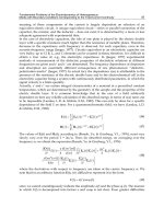
x of the crystal (Fig. 1):

E
1
= −(εε
0
)
−1
(∇∇+ k
2
0
)(ψ
1
p
0
),
H
1
= iω∇×(ψ
1
p
0
).
(55)
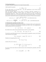
Also, when the direction of the dipole moment is perpendicular to the axis x, we obtain (Fig.
2):
⎧
⎪
⎪
⎨

⎪
⎪
⎩
E
2
= −
1
εε
0

k
2
0

p
⊥
ψ
0
+ ∇
⊥
∇(p
⊥
ψ
2
)

+ ∇∇(p
⊥
ψ
1

)

,
H
2
= −iω∇×

p
⊥
ψ
0
−e
x
∂
∂x
∇(p
⊥
ψ
2
)

(p
0
⊥p
⊥
).
(56)
Moreover, we note that the independent solutions (38) and (40) define the corresponding
polarization of electromagnetic waves. In addition, when ε
1

tends to ε, from (31) it follows
that the potential ψ
2
tends to zero and the well-known expressions of electromagnetic field
followed from formula (38) are obtained :
E
= iω(k
−2
0
∇∇+ 1)A, (57)
H
=(μμ
0
)
−1
∇×A, (58)
where the known vector potential of electromagnetic field for isotropic mediums is defined
from (51) as (24):
A
(r)=
μμ
0
4π

V
j(r

)
exp(ik
0

|r −r

|)
|r − r

|
dV. (59)
The obtained generalized solutions of the Maxwell equations are valid for any values of ε
1
and ε, as well as for sources of the electromagnetic waves, described by discontinuous and
singular functions.
Below as a specific application radiation from a Hertzian dipole in such a medium was
examined and the corresponding radiation patterns were presented.
11
The Generalized Solutions
of a System of Maxwell’s Equations for the Uniaxial Anisotropic Media
10 Electromagnetic Waves
(a) Case ε
1
= 9 (b) View in meridian surface
(c) Case ε
1
= 25 (d) View in meridian surface
Fig. 1. Directivity diagrams, the axis of dipole is parallel to axis of a crystal
It should be note that the pattern in Fig. 1 remains invariable, and independent of r.The
radiation pattern of the Hertzian dipole in isotropic medium is shown in Fig. 3, which of
course possesses rotation symmetry around x-axis.
Furthermore, we note here that the numerical calculation of the above solution of Maxwell
equations satisfies the energy conservation law. Poynting vector
< Π >=

1
2
Re
(E ×
¯
H
)
is necessary to calculate time-averaged energy-flux on spherical surface
Φ
=

s
sph
< Π
r
> dS,
12
Electromagnetic Waves Propagation in Complex Matter
The Generalized Solutions of a System of Maxwell’s Equations for the Uniaxial Anisotropic Media 11
(a) Case at r = 5, ε
1
= 7 (b) View in meridian surface
(c) Case at r = 5, ε
1
= 10 (d) View in meridian surface
Fig. 2. Directivity diagram, the axis of dipole (z) is perpendicular to axis of a crystal
Fig. 3. Directivity diagram of the Hertzian dipole, the isotropic medium (ε = ε
1
= 1)
which is a constant at various values of radius of sphere, where

¯
H is complex conjugate
function.
13
The Generalized Solutions
of a System of Maxwell’s Equations for the Uniaxial Anisotropic Media
12 Electromagnetic Waves
3.4 Directivity diagrams of the magnetic moment of a dipole in one-axis crystals
Exact analytical solution of Maxwell’s equations for radiation of a point magnetic dipole in
uniaxial crystals are obtained. Directivity diagrams of radiation of a point magnetic dipole
are constructed at parallel and perpendicular directions of an axis of a crystal.
On the basis of the obtained results (38) and (40), we will consider radiation of point magnetic
dipole moment in an uniaxial crystal. Let’s define intensity of an electromagnetic field for the
concentrated magnetic dipole at a parallel and perpendicular direction to a crystal axis in the
anisotropic medium and we will construct diagrams of directivity for both cases.
For a point radiator with the oscillating magnetic dipole moment
m
= np
m
e
−iωt
(p
m
= co n st) (60)
the electric current density is defined by using Dirac delta-function:
j
= −(m ×)δ( r). (61)
Components of a current density (61) are:
j
0

= e
x
(m
z
∂
∂y
−m
y
∂
∂z
)δ(r), (62)
j
⊥
= e
y
(m
x
∂
∂z
−m
z
∂
∂x
)δ(r)+e
z
(m
y
∂
∂x
−m

x
∂
∂y
)δ(r). (63)
It is possible to express the magnetic dipole moment m intheformofthesumoftwo
components of magnetic moment:
m
= m
0
+ m
⊥
, m
0
= e
x
m
x
. (64)
Relation between density of an electric current j
⊥
and the magnetic dipole moment m in the
anisotropic medium is defined from (63), in case m
= m
0
:
j
⊥
= m
x
(e

y
∂
∂z
−e
z
∂
∂y
)δ(r), (65)
∇j
⊥
= 0. (66)
3.4.1 The parallel directed magnetic momentum
Taking into account equality (66), from solutions (38) intensities of the electromagnetic field of
the magnetic dipole moment are defined, in the case when the magnetic dipole moment m is
directed parallel to the crystal axis x:

E
= −iμ
0
μω∇×(ψ
0
m
0
),
H
= −∇×∇×(ψ
0
m
0
).

(67)
It is necessary to notice, that expressions (67) correspond to the equations of an
electromagnetic field in isotropic medium (Fig. 4). In Fig. 4, directivity diagrams of magnetic
dipole moment in the case that the magnetic moment is directed in parallel to the crystal axis
are shown. The given directivity diagram coincides with the directivity diagram of a parallel
14
Electromagnetic Waves Propagation in Complex Matter
The Generalized Solutions of a System of Maxwell’s Equations for the Uniaxial Anisotropic Media 13
Fig. 4. Directivity diagram of the magnetic dipole, the isotropic medium (ε = ε
1
= 1)
directed electric dipole in isotropic medium. This diagram looks like a toroid, which axis is
parallel to the dipole axis. Cross-sections of the diagram are a contour on a plane passing
through an axis of the toroid. It has the shape of number ’eight’ ; cross-sections perpendicular
to the axis of the toroid represent circles.
3.4.2 The perpendicular directed magnetic momentum
Relation between density of an electric current j and the magnetic dipole momentum m
⊥
is
defined from expression (61), if it is directed on axis z:
j
= m
z
(e
x
∂
∂y
−e
y
∂

∂x
)δ(r). (68)
For the point magnetic dipole m
⊥
which is perpendicular to crystal axes, by substituting (68)
in solutions (40), we define components of field intensity (Fig. 5, Fig. 6):
⎧
⎪
⎪
⎪
⎪
⎪
⎪
⎪
⎨
⎪
⎪
⎪
⎪
⎪
⎪
⎪
⎩
E
x
= −iμ
0
μωm
z
∂ψ

1
∂y
,
E
y
= iμ
0
μωm
z
∂
∂x

ψ
0
+
∂
2
ψ
2
∂y
2

,
E
z
= iμ
0
μωm
z
∂

3
ψ
2
∂x∂y∂z
,
(69)
⎧
⎪
⎪
⎪
⎪
⎪
⎪
⎪
⎨
⎪
⎪
⎪
⎪
⎪
⎪
⎪
⎩
H
x
= −m
z
∂
2
ψ

0
∂x∂z
,
H
y
= −m
z
∂
2
∂y∂z

ψ
1
+
∂
2
ψ
2
∂x
2

,
H
z
= m
z

∂
2
∂y

2

ψ
1
+
∂
2
ψ
2
∂x
2

+
∂
2
ψ
0
∂x
2

.
(70)
In Figs. 5 and 6, directivity diagrams of the magnetic moment of a dipole perpendicular
a crystal axis at different values of radius are shown, for two (30) values of dielectric
permeability ratio, ε
1
/ε = 9andε
1
/ε = 15 . The magnetic dipole is directed along an axis z (a
15

The Generalized Solutions
of a System of Maxwell’s Equations for the Uniaxial Anisotropic Media
14 Electromagnetic Waves
(a) Case r = 3 (b) View in meridian surface r = 3, ϕ = π/2
(c) Case at r = 9 (d) View in meridian surface r = 9, ϕ = π/2
Fig. 5. Directivity diagram, the axis of magnetic dipole (z) is perpendicular to axis of a crystal
at ε
1
/ε = 9
(a) Case r = 1 (b) View in meridian surface r = 1, ϕ = π/2
(c) Case at r = 5 (d) View in meridian surface r = 5, ϕ = π/2
Fig. 6. Directivity diagram, the axis of magnetic dipole (z) is perpendicular to axis of a crystal
at ε
1
/ε = 15.
crystal axis - along x). As one can see from Fig. 5, that radiation in a direction of the magnetic
moment does not occur, it propagates in a direction along an axis of a crystal.
Validity of solutions has been checked up on performance of the conservation law of energy.
Time-averaged energy flux of energy along a surface of sphere for various values of radius
was calculated for this purpose. Numerical calculations show that energy flux over the above
mentioned spherical surfaces, surrounding the radiating magnetic dipole, remains constant,
which means that energy conservation is preserved with high numerical accuracy.
16
Electromagnetic Waves Propagation in Complex Matter
The Generalized Solutions of a System of Maxwell’s Equations for the Uniaxial Anisotropic Media 15
The obtained generalized solutions of the Maxwell equations are valid for any values of ε
1
and
ε, and also for any kind of sources of the electromagnetic waves, described by discontinuous
and singular functions.

4. Radiation of electric and magnetic dipole antennas in magnetically anisotropic
media
The electric and magnetic field intensities satisfy the system of stationary Maxwell’s equations
(1) which is possible to be presented in matrix form (4), where
M
=

−iωε
0
εIG
0
G
0
iωμ
0
ˆ
μ

,
ˆ
μ
=
⎛
⎝
μ 00
0 μ 0
00μ
1
⎞
⎠

. (71)
M is Maxwell’s operator and μ represents the magnetic permeability.
In magnetically anisotropic media the relation between induction and intensity of the
magnetic field is:
B
= μ
0
ˆ
μH, B
x
= μ
0
μH
x
, B
y
= μ
0
μH
y
, B
z
= μ
0
μ
1
H
z
. (72)
The elements of the magnetic permeability tensor

ˆ
μ are chosen so that the axis of anisotropy
is directed along axis z. It is required to define the intensities of the electromagnetic field E, H
in the space of generalized functions.
4.1 Solution of the problem
By means of direct Fourier transformation we write down the system of the equations in
matrix form (9). The solution of this problem is reduced to the solution of the system, where
˜
U is defined by means of inverse matrix
˜
M
−1
.
By introducing new functions according to
˜
ψ
m
1
=
1
k
2
n
−k
2
x
−k
2
y
−

μ
1
μ
k
2
z
, (73)
˜
ψ
m
2
=

μ
1
μ
−1

˜
ψ
m
1
˜
ψ
0
, (74)
the components of the electromagnetic field after transformations in spectral domain can be
written as follows:
⎧
⎪

⎪
⎪
⎨
⎪
⎪
⎪
⎩
˜
E
x
=(iεε
0
ω)
−1

k
2
0

˜
j
x
˜
ψ
0
+ k
y
(k ×
˜
j)

z
˜
ψ
m
2

−k
x
k
˜
j
˜
ψ
0

,
˜
E
y
=(iεε
0
ω)
−1

k
2
0

˜
j

y
˜
ψ
0
−k
x
(k ×
˜
j)
z
˜
ψ
m
2

−k
y
k
˜
j
˜
ψ
0

,
˜
E
z
=(iεε
0

ω)
−1
(k
2
0
˜
j
z
−k
z
˜
j)
˜
ψ
0
,
(75)
⎧
⎪
⎨
⎪
⎩
˜
H
x
= −i

(k ×
˜
j

)
x
˜
ψ
0
+ k
x
k
z
(k ×
˜
j
)
z
˜
ψ
m
2

,
˜
H
y
= −i

(k ×
˜
j
)
y

˜
ψ
0
+ k
y
k
z
(k ×
˜
j
)
z
˜
ψ
m
2

,
˜
H
z
= −i(k ×
˜
j)
z
˜
ψ
m
1
,

(76)
17
The Generalized Solutions
of a System of Maxwell’s Equations for the Uniaxial Anisotropic Media
16 Electromagnetic Waves

(k ×
˜
j)
z
≡ k
x
˜
j
y
−k
y
˜
j
x

.
It is possible to represent the electromagnetic fields in (75) and (76) in vector form as following
˜
E
=(iεε
0
ω)
−1


k
2
0

˜
j
˜
ψ
0
+ k × e
z
(k ×
˜
j
⊥
)
z
˜
ψ
m
2

−k(k
˜
j)
˜
ψ
0

, (77)

˜
H
= i(e
z
k
z
−k)k
z
(k ×
˜
j
⊥
)
z
˜
ψ
m
2
+ ie
z
(k ×
˜
j
⊥
)
z
(
˜
ψ
0

−
˜
ψ
m
1
) −ik ×
˜
j
˜
ψ
0
, (78)
where
˜
j
=
˜
j
⊥
+
˜
j
0
,
˜
j
0
=(0, 0,
˜
j

z
),
˜
j
⊥
=(
˜
j
x
,
˜
j
y
,0), k
2
0
= ω
2
ε
0
εμμ
0
, k
2
n
= k
2
0
μ
1

μ
.
It should be noted that the following useful formulae follow from (12), (73) and (74):
˜
ψ
0
−
˜
ψ
m
1
=(k
2
0
−k
2
z
)
˜
ψ
m
2
, (79)
˜
ψ
0
−
μ
1
μ

˜
ψ
m
1
=(k
2
x
+ k
2
y
)
˜
ψ
m
2
. (80)
With the help of identity in (79) and (80), the last equation (78) can be represented as
˜
H
= i(k
2
0
e
z
−k
z
k)(k ×
˜
j
⊥

)
z
˜
ψ
m
2
−i(k ×
˜
j)
˜
ψ
0
. (81)
Using the property of convolution (17) and considering inverse Fourier transformation it is
possible to get the solution of the Maxwell equations in form (18).
So, after the inverse Fourier transformations from (77) and (81) we obtain:
E
=(iεε
0
ω)
−1

(k
2
0
+ ∇∇)j ∗ ψ
0
−k
2
0

∇×

e
z
(∇×j
⊥
)
z

∗ ψ
m
2

, (82)
H
=(k
2
0
e
z
+
∂
∂z
∇)(∇×j
⊥
)
z
∗ψ
m
2

−∇×j ∗ψ
0
. (83)
This solution can be written in the form of the sum of two solutions:
E
= E
1
+ E
2
, H = H
1
+ H
2
.
It should be noted that the first of them is the ’isotropic’ solution. It is defined by Green’s
function ψ
0
and the density of the current j
0
directed parallel to axis z (of the anisotropy):

E
1
=(iεε
0
ω)
−1
(∇∇+ k
2
0

)(ψ
0
∗j
0
),
H
1
= −∇×(ψ
0
∗j
0
),
(84)
where ψ
0
is the Green’s function (22). The second solution can be written by using the
component of the density of the current j
⊥
perpendicular to axis z and the Green’s functions
ψ
0
and ψ
m
2
:
⎧
⎪
⎪
⎨
⎪

⎪
⎩
E
2
= −
i
εε
0
ω

(k
2
0
+ ∇∇)j
⊥
∗ψ
0
−k
2
0
∇×

e
z
(∇×j
⊥
)
z

∗ψ

m
2

,
H
2
=(k
2
0
e
z
+
∂
∂z
∇)(∇×j
⊥
)
z
∗ ψ
m
2
−∇×j
⊥
∗ψ
0
,
(85)
18
Electromagnetic Waves Propagation in Complex Matter
The Generalized Solutions of a System of Maxwell’s Equations for the Uniaxial Anisotropic Media 17

ψ
m
1
= F
−1
[
˜
ψ
m
1
]=−
1
4π

μ
μ
1
exp(ik
n
r

)
r

, (86)
ψ
m
2
=(
μ

μ
1
−1)ψ
0
∗ψ
m
1
, (87)
r

=

x
2
+ y
2
+
μ
μ
1
z
2
. (88)
Furthermore, the following transformation is valid similarly to (45):
F
−1
[
˜
ψ
m

2
]=F
−1
[
˜
ψ
0
(k
2
0
−k
2
z
)
−1
] − F
−1
[
˜
ψ
m
1
(k
2
0
−k
2
z
)
−1

].
We find that function ψ
m
2
, Eqn. (87) is given by:
ψ
m
2
= −
i
8πk
0

e
ik
0
z

Ci
(k
0
(r −z)) + isi(k
0
(r −z))

+ e
−ik
0
z


Ci
(k
0
(r + z)) +isi(k
0
(r + z))

−
−
e
ik
0
z

Ci
(k
n
r

−k
0
z)+isi (k
n
r

−k
0
z)

−e

−ik
0
z

Ci
(k
n
r

+ k
0
z)+isi (k
n
r

+ k
0
z)


.
(89)
It should be noted that ψ
2
and ψ
m
2
are similar for magnetic and dielectric crystals.
4.2 Radiation patterns o f Hertzian radiator in magnetically anisotropic media
On the basis of the results obtained above, we consider now numerical results for the radiation

of the electric dipole.
The dipole moment of point electric dipole is given by p , Eqn. (52). It corresponds to the
current density defined by means of the Dirac delta-function (53).
The expression of the electromagnetic field for electric radiator will take the following form
as for isotropic medium, when the direction of the dipole moment is parallel to the axis z
(p = p
0
) (Fig. 7):

E
1
= −(iεε
0
)
−1
(∇∇+ k
2
0
)(ψ
0
p
0
),
H
1
= iω∇×(ψ
0
p
0
).

(90)
Also when the direction of the dipole moment is perpendicular to axis z, we obtain
(p = p
⊥
)
(Fig. 8, Fig. 9):
⎧
⎨
⎩
E
2
=(εε
0
)
−1
(k
2
0
∇×

e
z
(∇×p
⊥
ψ
m
2
)
z


−

k
2
0
+ ∇∇)(p
⊥
ψ
0
)

,
H
2
=(k
2
0
e
z
+
∂
∂z
∇)(∇×p
⊥
ψ
m
2
)
z
−∇×(p

⊥
ψ
0
).
(91)
4.3 Radiation patterns of point ma gnetic dipole in magnetically anisotropic media
On the basis of the obtained results, we consider now radiation of point magnetic dipole
moment. For a point radiator with the oscillating magnetic dipole moment, similarly to the
magnetic dipole case in one-axis crystals, Eqn. (60), the electric current density is defined by
using Dirac’s delta-function, Eqn. (61). It is possible to express the magnetic dipole moment
m in the form of the sum of two components of magnetic moment:
m
= m
0
+ m
⊥
, m
0
= e
z
m
z
. (92)
19
The Generalized Solutions
of a System of Maxwell’s Equations for the Uniaxial Anisotropic Media
18 Electromagnetic Waves
Fig. 7. Directivity diagram. Electric dipole moment is parallel to the axis z (p = p
0
)

(a) Case r = 3 (b) View in meridian surface r = 3, ϕ = π/2
(c) Case r = 9 (d) View in meridian surface r = 9, ϕ = π/2
Fig. 8. Directivity diagram. The axis of electric dipole is perpendicular to axis z (p = p
⊥
),
μ
1
/μ = 9
Components of a current density, Eqn. (61), have the following form:
j
0
= e
z
(m
y
∂
∂x
−m
x
∂
∂y
)δ(r), (93)
and
j
⊥
=

e
x
(m

z
∂
∂y
−m
y
∂
∂z
)+e
y
(m
x
∂
∂z
−m
z
∂
∂x
)

δ
(r). (94)
Case m
= m
0
.
Relation between density of an electric current j
⊥
and the magnetic dipole moment is defined
from (93) in case when the magnetic dipole moment m is directed lengthwise z:
j

⊥
= m
z
(e
x
∂
∂y
−e
y
∂
∂x
)δ(r). (95)
20
Electromagnetic Waves Propagation in Complex Matter
The Generalized Solutions of a System of Maxwell’s Equations for the Uniaxial Anisotropic Media 19
(a) Case r = 1 (b) View in meridian surface r = 1, ϕ = π
(c) Case r = 5 (d) View in meridian surface r = 5, ϕ = π
Fig. 9. Directivity diagram. The axis of electric dipole is perpendicular to axis z (p = p
⊥
),
μ
1
/μ = 15
It should be noted that the following useful formula hold:
∇j
⊥
= 0, j
0
= 0. (96)
Taking into account (96), intensities of the electromagnetic field by the magnetic dipole

moment are defined from the solutions (85) in this case, as following :
⎧
⎪
⎨
⎪
⎩
E
= −iμ
0
μ
1
ωm
0
∇×(e
z
ψ
m
1
),
H
= m
0
ψ
m
1
+ m
0
(
μ
1

μ
−1)
∂
2
∂z
2
ψ
m
1
−m
0
μ
1
μ
∂
∂z
∇ψ
m
1
.
(97)
We have taken advantage of the next formulae which followed from (79) after inverse Fourier
transformation
μ
1
μ
ψ
m
1
= ψ

0
+(
∂
2
∂x
2
+
∂
2
∂y
2
)ψ
m
2
, (98)
ψ
0
= ψ
m
1
+(
∂
2
∂z
2
+ k
2
0
)ψ
m

2
. (99)
Directional diagrams are represented in Fig. 10.
Case m
= m
⊥
.
For the point magnetic dipole moment m
⊥
which is perpendicular to axis z, by substituting
(61) ( or (93) and (94)) in (84) and (85), we define intensities of electromagnetic field as
following (Fig. 11, Fig. 12):
⎧
⎪
⎪
⎨
⎪
⎪
⎩
E
= iμ
0
μω

∂
∂z
{m
⊥
×e
z

μ
1
μ
ψ
m
1
−∇
⊥
(∇×ψ
m
2
m
⊥
)
z
}−e
z
(∇×ψ
0
m
⊥
)
z

,
H
=(k
2
0
e

z
+
∂
∂z
∇)
∂
∂z
∇(m
⊥
ψ
m
2
) −∇×∇×(m
⊥
ψ
0
).
(100)
21
The Generalized Solutions
of a System of Maxwell’s Equations for the Uniaxial Anisotropic Media
20 Electromagnetic Waves
(a) Case μ
1
/μ = 7 (b) View in meridian surface (ϕ = 0)
Fig. 10. Directivity diagram. The axis of magnetic dipole is parallel to axis z (m = m
0
)
(a) Case r = 5 (b) View in meridian surface r = 5, ϕ = π/2
(c) Case r = 10 (d) View in meridian surface r = 10, ϕ = π/2

Fig. 11. Directivity diagram. The axis of magnetic dipole is perpendicular to z, μ
1
/μ = 7
(a) Case r = 5 (b) View in meridian surface r = 6, ϕ = π/2
(c) Case r = 10 (d) View in meridian surface r = 10, ϕ = π/2
Fig. 12. Directivity diagram. The axis of magnetic dipole is perpendicular to z, μ
1
/μ = 15
The numerical calculation of the solution of Maxwell equations satisfies the energy
conservation law. Numerical computation shows that time average value energy flux on a
22
Electromagnetic Waves Propagation in Complex Matter
The Generalized Solutions of a System of Maxwell’s Equations for the Uniaxial Anisotropic Media 21
surface of sphere from a point dipole remains independent from its radius, with very high
accuracy. As shown in the electric dipole directional diagrams, medium becomes isotropic for
such radiator if its moment is directed along anisotropy axis.
The dipole pattern in isotropic media is shown in Fig. 1 and directional diagram itself
possesses the rotation symmetry. However the point magnetic moment does not possess such
property.
When μ
1
approaches μ, the potential ψ
2
tends to zero and the well-known expressions of
electromagnetic field in form (57), (58) and (59) follow from (84) and (85).
The obtained generalized solutions of the Maxwell equations are valid for any values of μ
1
and μ, also near the sources of the electromagnetic waves, described by discontinuous and
singular functions.
5. Conclusion

We were able to solve Maxwell’s equations for uniaxial anisotropic medium actually showing
that the exact general solution in vector form is given by integral convolutions of the
fundamental solutions ψ
0
, ψ
1
and ψ
2
with external arbitrary current density, without using
the scaling procedure to a corresponding vacuum field and the dyadic Green’s functions. In
the particular case of a current density, the radiation field of a dipole is considered in greater
detail. That method may be useful in analytical treatment of corresponding boundary value
problems.
6. Acknowledgment
I wish to thank Professor Panayiotis Frangos, School of Electrical and Computer Engineering,
National Technical University of Athens, Greece, for providing me with the encouragement
to pursue research in this field.
7. References
Alekseyeva, L. A. & Sautbekov, S. S. (1999). Fundamental Solutions of Maxwell’s Equations.
Diff. Uravnenia,Vol. 35, No. 1, 125-127.
Alekseyeva, L. A. & Sautbekov, S. S. (2000). Method of Generalized Functions For Solving
Stationary Boundary Value Proplems For Maxwell’s Equations. Comput. Math. and
Math. Phys., Vol. 40, No. 4, 582-593.
Barkeshli, S. (1993). An efficient asymptotic closed-form dyadic Green’s function for grounded
double-layered anisotropic uniaxial material slabs, J. Electromagnetic Waves and
Applications, Vol. 7, No. 6, 833-856.
Born, M. & Wolf, E. (1999). Principles of Opti cs. Electromagnetic Theory of Propagation, Interference
and Dffraction of Light, 7th ed. Cambridge U. Press, Cambridge.
Bunkin, F.V. (1957). On Radiation in Anisotropic Media. Sov. Phys. JETP Vol. 5, No.2, 277-283.
Chen, H. C. (1983). Theory of Electromagnetic Waves, McGraw-Hill, New York.

Clemmow, P.C. (Jun. 1963a). The theory of electromagnetic waves in a simple anisotropic
medium, Proc. IEE, pp. 101-106, Vol. 110, No. 1, Jun 1963.
Clemmow, P.C. (Jun. 1963b). The resolution of a dipole field in transverse electric and
transverse magnetic waves, Proc. IEE, pp. 107-111, Vol. 110, No. 1, Jun 1963.
23
The Generalized Solutions
of a System of Maxwell’s Equations for the Uniaxial Anisotropic Media
22 Electromagnetic Waves
Cottis, P. G. & Kondylis, G. D. (Feb. 1995). Properties of the dyadic Green’s function for an
unbounded anisotropic medium, IEEE Trans. Ant. Prop., Vol. 43, No. 2, Feb. 1995,
154-161.
Kogelnik, H. & Motz, H. (1963). Electromagnetic Radiation from Sources Embedded in an
Infinite Anisotropic Medium and the Significance of the Poynting Vector, Proc. S ymp.
on Electromagnetic Theory and Antennas, pp. 477-493, 1963, Pergamon Press, New York.
Kong, J. A. (1986). Electromagnetic Wave Theory, The 2nd ed., John Wiley and Sons, New York.
Lee, J. K. & Kong, J. A. (1983). Dyadic Green’s functions for layered anisotropic medium.
Electromagnetics, Vol. 3, 111-130.
Ren, W. (Jan. 1993). Contributions to the Electromagnetic Wave Theory of Bounded
Homogeneous Anisotropic Media. Physical Review E, Vol. 47, No. 1, 664-673.
Sautbekov, S.; Kanymgazieva, I. & Frangos, P. (2008). The generalized solutions of Maxwell
equations for the uniaxial crystal, Journal of Applied Electromagnetism (JAE), Vol. 10,
No. 2, 43-55, ISSN 1392-1215.
Uzunoglu, N. K.; Cottis, P. G. & Fikioris, J. G. (Jan. 1985). Excitation of Electromagnetic Waves
in a Gyroelectric Cylinder, IEEE Trans. Ant. Propa., Vol. AP-33, No. 1, 90-99.
Vladimirov, V. S. (2002). Methods of the theory of generalized functions, Taylor and Francis, ISBN
0-415-27356-0, London.
Weiglhofer, W. S. (Feb. 1990). Dyadic Greens functions for general uniaxial media, IEE Proc.
H., Vol. 137, No. 1, 5-10.
Weiglhofer, W. S. (1993). A dyadic Green’s function representation in electrically gyrotropic
media, AE

¨
U, Vol. 47, No. 3, 125-130.
24
Electromagnetic Waves Propagation in Complex Matter
2
Fundamental Problems of the Electrodynamics
of Heterogeneous Media with Boundary
Conditions Corresponding to
the Total-Current Continuity
N.N. Grinchik
1
, O.P. Korogoda
2
, M.S. Khomich
2
, S.V. Ivanova
3
,
V.I. Terechov
4
and Yu.N. Grinchik
5

1
A.V. Luikov Heat and Mass Transfer Institute
of the National Academy of Science, Minsk,
2
Scientific-Engineering Enterprise “Polimag”, Minsk,
3
National Research Nuclear University "MEPhI", Moscow,

4
Thermal Physics Institute, Novosibirsk,
5
Belarusian State University, Minsk,
1,2,5
Republic of Belarus
3,4
Russian Federation
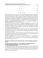
1. Introduction
Let us consider the interface S between two media having different electrophysical
properties. On each of its side the magnetic-field and magnetic-inductance vectors as well as
the electric-field and electric-displacement vectors are finite and continuous; however, at the
surface S they can experience a discontinuity of the first kind. Furthermore, at the interface
there arise induced surface charges σ and surface currents i (whose vectors lie in the plane
tangential to the surface S) under the action of an external electric field.
The existence of a surface charge at the interface S between the two media having different
electrophysical properties is clearly demonstrated by the following example. We will consider
the traverse of a direct current through a flat capacitor filled with two dielectric materials
having relative permittivities ε
1
and ε
2
and electrical conductivities λ
1
and λ
2
. A direct-current
voltage U is applied to the capacitor plates; the total resistance of the capacitor is R (Fig. 1). It is
necessary to calculate the surface electric charge induced by the electric current.
From the electric-charge conservation law follows the constancy of flow in a circuit;

therefore, the following equation is fulfilled:



12
12
/
nn
EEURS


(1)
where
1
n
E and
2
n
E are the normal components of the electric-field vector.
At the interface between the dielectrics, the normal components of the electric-inductance
vector change spasmodically under the action of the electric field by a value equal to the
value of the induced surface charge σ:

Electromagnetic Waves Propagation in Complex Matter

26

12
01 02nn
EE





(2)


Fig. 1. Dielectric media inside a flat capacitor
Solving the system of Eqs. (see Equations 1 and 2), we obtain the expression for σ







011 22
///URS





(3)
It follows from (see Equation 3) that the charge σ is determined by the current and the
multiplier accounting for the properties of the medium. If






11 22
//0
 

 (4)
a surface charge σ is not formed. What is more, recent trends are toward increased use of
micromachines and engines made from plastic materials, where the appearance of a surface
charge is undesirable. For oiling of elements of such machines, it is best to use an oil with a
permittivity
oil

satisfying the relation

12oil



 (5)
This oil makes it possible to decrease the electrization of the moving machine parts made
from dielectric materials. In addition to the charge σ, a contact potential difference arises
always independently of the current.
An electric field interacting with a material is investigated with the use of the Maxwell
equation (1857)

,
total


  jHD

(6)

,0
t


  

B
EB
(7)
where
00
;;
total
t

 

  

D
j
EBHDE
. In this case, at the interface S the above system of
equations is supplemented with the boundary conditions (Monzon, I.; Yonte,T.; Sanchez-
Soto, L., 2003; Eremin,Y. & Wriedt,T., 2002)