Electromagnetic Waves Propagation in Complex Matter Part 9 pptx

Electromagnetic Waves in Contaminated Soils

147



.4 .85 1.3 1.75 2.2
0
0.005
0.01
0.015
0.02
0.025
0.03
0.035
0.04
0.045
0.05
Frequency (GHz)
Amplitude (V/m)




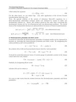
Fig. 14. Experimental frequency-response in water-saturated background soil
cable and the bottom of the receiving antenna. Therefore, it needs to be adjusted for this
difference.
Up to this point, the FDTD travel-time (
t
3

– t
1
) from the feed cable to the tip of the receiving
antenna is computed. The travel time through the receiving antenna (
t
4
– t
3
), which is by
symmetry equal to (
t
2
– t
1
), should be added to (t
3
– t
1
) to find the total travel time between
the feed and receiver cables (
t
4
– t
1
) for the FDTD model. The resulting travel time from the
FDTD simulation can be used for comparison with the experimental results.
The travel time computed from the forward model is
(4500 + 900 - 1000) × 2 psec = 8.8 nsec,
which closely agrees with the one indirectly computed from the experimentally collected
frequency-response data:

(5700 - 1000) × 1.87 psec = 8.6 nsec. The difference is due to the
slight, potential discrepancy between the dielectric constant assigned to the forward model
(used from the results of another work by the authors (Zhan et al., 2007)) and the real values
of the experimentation.
The intensities of the unprocessed received signals from the FDTD simulation (Fig. 13(a))
and experimentation (Fig. 15(a)) agree relatively well, but not perfectly. The reason is the
potential slight discrepancy between the electrical conductivity assigned to the FDTD model
compared to the actual one of the experiment. However, due to the difference between the
necessary processing methods (different filters), the intensity of the processed received
signals for the FDTD simulation (Fig. 13(b)) and the one of the experiment (Fig. 15(b)) do not
agree as closely.
This comparison consists of the incident field for the homogeneous background soil. The
comparison for the total and scattered fields at the presence of any anomalies (e.g., dielectric
objects) will be conducted in the future.

Electromagnetic Waves Propagation in Complex Matter

148



0 2000 4000 6000 8000 10000
-4
-3
-2
-1
0
1
2
3

4
x 10
-3
Time
(
x 2
p
sec
)
Amplitude (V/m)



(a)

0 1000 2000 3000 4000 5000 6000 7000 8000 9000 10000
-2
0
2
4
6
8
10
x 10
-4
Time (x 1.87psec)
Amplitude (V/m)


(b)

Fig. 15. Received signal (
E
z4
) at the top of the receiver in the saturated background, indirectly
computed from the experimental frequency-response: a) Unprocessed, and b) Processed.

Electromagnetic Waves in Contaminated Soils

149
7. Conclusion
A finite difference time domain (FDTD) model was developed for monopole and dipole
antennae. Then, the scattering due to dielectric materials (to simulate DNAPL pools) in soils
was modeled and analyzed. Results of the two simulated cases using the FDTD model
demonstrate strong perturbation by the DNAPL pool on the electric field in the fully water-
saturated sandy soil. In the case of the monopole antenna, the DNAPL pool target is more
visible on the X and Y components of the electric field compared to the major component Z.
The perturbation on the intensity of the electric field (|E|) transmitted by the monopole
antenna is not as strongly visible as in the dipole case. In the dipole case, X and Y
components are those parallel to likely hydraulic-conductivity contrast planes (
e.g., usually
horizontal clay lenses within a thick sand layer), which are potential locations to accumulate
DNAPLs.
Different components of the electric field can selectively be collected using receiving
antennae with different polarizations from the polarization of the transmitting antenna (
e.g.,
a horizontally-polarized receiving monopole antenna and a vertically-polarized transmitting
monopole antenna). Therefore, designing the receiving antenna alignment and polarization
to selectively collect electric field components parallel to a possible DNAPL pool may help
to compensate for a stronger perturbation on the minor components (X and Y) of the electric

field emitted from a Z-polarized monopole antenna. These minor components should be of a
high enough signal to noise ratio.
In the case of the dipole antenna, all three components of the electric field in the fully water-
saturated soil have almost equal detection potential. In both of the above cases, there is a
strong dielectric contrast between the DNAPL pool and the water-saturated soil. However,
different radiation patterns of the dipole antenna compared to the monopole antenna may
make the dipole antenna more desirable for DNAPL detection.
Field problems can be scaled down in size along with scaling up the frequency in non-
dispersive soils to achieve the proper geometry and frequency for simulation purposes. This
linear scaling of frequency and size may not work as well for dispersive soils, since
frequency-dependent dielectric properties of dispersive soils add nonlinearity to the scaling
problem. Other conclusions follow.

Images provided by such simulations show the field distribution that exists throughout
the subsurface (i.e., similar to filling the entire volume with receiver antennae), but the
field can only be observed practically by placing a reasonable number of receiving
antennae at key underground positions with the appropriate polarization. This research
can be used to find the radiation patterns of different antenna types and the interaction
of the radiated field with soil heterogeneities, which leads to a better understanding of
subsurface wave behavior at these key positions and aids the selection of optimum
antenna patterns to cover these key positions.

While the depth of contamination is a problem for surface-reflection methods (e.g.,
GPR), there are no theoretical depth limitations for CWR, except practical drilling
limitations and cost. The separation limitations between transmitting and receiving
antennae used for CWR still exist. However, CWR has the advantage of using a
one-way traveling path (transmission), unlike the two-way traveling path of surface-
reflection GPR. In addition, the strong reflecting air-soil interface in the

Electromagnetic Waves Propagation in Complex Matter

150
surface-reflection GPR technique is eliminated in the CWR technique and replaced
with a better-controlled coupling between the borehole antennae and surrounding
soil.

The perturbation due to the DNAPL target is stronger for the greater dielectric
permittivity contrast between DNAPL pools and highly moist soil, as opposed to
DNAPL plumes with low DNAPL saturation and dryer soils.

The signal to noise ratio of the scattered field by DNAPL pools should be high enough
for measurements. As seen in the figures, the scattered field is comparable to the
incident field. Therefore, if the signal to noise ratio of the incident field is high enough
for measurement, the scattered field will probably have a large enough signal to noise
ratio to be measurable as well.

The results of this forward model with monopole and dipole antennae show that the
field perturbation (scattered = total - incident) for relatively large DNAPL pools at high
enough DNAPL saturation, is of the same order of magnitude as the incident signal.
This proves DNAPL detection using CWR in water-saturated soils feasible. The
simulation tool can also be used as a forward model to develop an inverse scheme for
DNAPL imaging.

Armed with the background data as well as the radiation patterns of different antennae
(via simulations like those in this chapter), the existence of DNAPL pools can be
confirmed with efficient inverse models and judicious placement of receiving antennae
(i.e., pattern of antenna installation) where stronger perturbation and reception by
receiving antennae are expected.
CWR may be a feasible and reasonable method to monitor DNAPL pools in a suitable
environment. This most suitable environment is a medium consisting of a low-loss, low-

heterogeneity porous material. In other media, it is more difficult to distinguish DNAPL
accumulation from geologic variations, which are more complicated due to heterogeneity.
Nevertheless, soil heterogeneity may not pose a crucial problem under water-saturated
conditions since different soils behave similarly at relatively high degrees of water-
saturation and high frequencies (the case is different for low frequencies). Monitoring
DNAPL movement may well be possible or easier in an even less saturated heterogeneous
environment because of the static nature of stratigraphic events and the dynamic nature of
DNAPL flow. Several features of DNAPL pools may help to distinguish them from
stratigraphic events, such as their irregular shapes with sharp lateral boundaries.
Finally, the FDTD model was compared for the incident field due to the monopole case in a
homogeneous water-saturated sandy soil background with the experimental results. The
reasonable agreement between both the travel time and intensity of the unprocessed,
simulated and experimental results validates the FDTD model. The comparison and
validation for the total and scattered fields at the presence of any anomalies (e.g., dielectric
objects) need to be studied in the future.
8. Acknowledgement
This research was supported in part by the Gordon Center for Subsurface Sensing and
Imaging Systems (CenSSIS), under the Engineering Research Centers Program of the
National Science Foundation (NSF: Award Number EEC-9986821).

Electromagnetic Waves in Contaminated Soils

151
The authors would like to express gratitude for financial and scientific support provided by
the Gordon CenSSIS and NSF.
9. References
Ajo-Franklin, J. B., Geller, J. T. & Harris, J. M. (2004). The dielectric properties of granular
media saturated with DNAPL/water mixtures.
Geophysical Research Letters (GRL),
Vol. 31, No. 17, L17501

Anderson, J. & Peltola, J. (1996).
Ground Penetrating Radar as a tool for detecting contaminated
areas: Groundwater Pollution Premier
, CE 4594 Soil and Groundwater Pollution, Civil
Engineering Department, Virginia Tech., Date of Access: Feb/2011, Available from:
< />/gprjp.html#Intro>
Arulanandan, K. (1964). Dielectric method for prediction of porosity of saturated soils.
ASCE
Journal of Geotechnical Engineering
, Vol. 117, No. 2, pp. 319-330
Arulanandan, K. & Smith, S. S. (1973). Electrical dispersion in relation to soil structure.
ASCE Journal of Soil Mechanics and Foundation Div., Vol. 99, No. 12, pp. 1113-
1133
Balanis, C. A. (1989).
Advanced engineering electromagnetic, John Wiley & Sons, New York,
1008p
Belli, K., Rappaport, C., Zhan, H. & Wadia-Fascetti, S. (2009). Effectiveness of 2D and 2.5D
FDTD Ground Penetrating Radar Modelling for Bridge Deck Deterioration
Evaluated by 3D FDTD.
IEEE Transactions on Geoscience and Remote Sensing, Vol. 47,
No. 11, pp. 3656 - 3663.
Belli, K., Rappaport, C. & Wadia-Fascetti, S. (2009a). Forward Time Domain Ground
Penetrating Radar Modelling of Scattering from Anomalies in the Presence of
Steel Reinforcements.
Research in Nondestructive Evaluation, Vol. 20, No. 4, pp.
193 - 214.
Binley, A., Winship, P. & Middleton, R. (2001). High resolution characterization of vadose
zone dynamics using Cross-Borehole Radar.
Water Resource Research, Vol. 37, no. 11,
pp. 2639-2652

Blackhawk Geoservices Inc. (2008).
Integrated geophysical detection of DNAPL source zones,
Final Report, Date of Access: Feb/2011, Available from:
<
Bradford, J. H. & Wu, Y. (2007). Instantaneous spectral analysis; time-frequency mapping
via wavelet matching with application to 3D GPR contaminated site
characterization.
The Leading Edge, Vol. 26, pp. 1018-1023
Brewster, M. L. & Annan, A. P. (1994). GPR monitoring of a controlled DNAPL release, 200
MHz radar.
Geophysics, Vol. 59, No. 8, pp. 1211-1221
Daniels, J. J., Roberts, R. & Vendl, M. (1992). Site studies of Ground Penetrating Radar for
monitoring petroleum product contaminants.
Proceedings of SAGEEP (Symposium of
the Applications of Geophysics to Engineering and Environmental Problems)
, Society of
Engineering Mine Exploration, pp. 597–609

Electromagnetic Waves Propagation in Complex Matter

152
Dobson, M. C., Ulaby, F. T., Hallikainen, M. T. & El-Rayes, M. A. (1985). Microwave
dielectric behavior of wet soil, Part II: Dielectric mixing models.
IEEE Transaction on
Geoscience and Remote Sensing
, GE- 23, No. 1, pp. 35–46
Farid, A. M., Alshawabkeh, A. N. & Rappaport, C. M. (2006). Calibration and Validation of a
Laboratory Experimental Setup for CWR in Sand.
ASTM, Geotechnical Testing
Journal

, Vol. 29, Issue 2, pp. 158-167
Firoozabadi, R., Miller, E., Rappaport, C. & Morgenthaler, A. (2007). A New Inverse Method
for Subsurface Sensing of Object under Randomly Rough Ground Using Scattered
Electromagnetic Field Data.
IEEE Transactions on Geoscience and Remote Sensing, Vol.
45, No. 1, pp. 104-117.
Gandhi, O. (1993). A frequency dependent FDTD (Finite Difference Time Domain)
formulation for general dispersive media.
IEEE Transactions on Microwave Theory
and Techniques
, Vol. 41, pp. 658-665
Geller, J. T., Kowalsky, M. B., Seifert, P. K. & Nihei, K. T. (2000). Acoustic detection of
immiscible liquids in sand.
Geophysical Research Letters, Vol. 27, No. 3, pp. 417-420,
2000
Grant, I. S. & Philips, W. R. (1990).
Electromagnetism, John Wiley & Sons, New York, 525
pp
Grimm, R. & Olhoeft, G. (2004). Cross-hole complex resistivity survey for PCE at the
SRS A-014 outfall.
Proceedings of SAGEEP, Colorado Springs, Colorado, 2004,
pp. 455-464
Hallikainen, M. T., Ulaby, F. T., Dobson, M. C., El-Rayes, M. A. & Lin-Kun, W. (1985).
Microwave dielectric behavior of wet soil: Part I- Empirical models and
experimental observations.
IEEE Transaction on Geoscience and Remote Sensing, GE-
23, No. 1, pp. 25–34
Hipp, J. (1974). Soil electromagnetic parameters as functions of frequency, soil density, and
soil moisture.
Proceedings of IEEE, Vol. 62, No.1, pp. 98-103

Hoekstra, P. & Doyle, W. T. (1971). Dielectric relaxation of surface adsorbed water.
Journal of
Colloid and Interface Science
, Vol. 36, No. 4, pp. 513-521
Hoekstra, P. & Delaney, A. (1974). Dielectric properties of soils at UHF and microwave
frequencies.
Journal of Physics Research, Vol. 79, No. 11, pp. 1699–1708
Interstate Technology and Regulatory Cooperation (ITRC) (2000).
Work Group
DNAPLs/Chemical Oxidation Work Team, Dense Non-Aqueous Phase Liquids (DNAPLs)
,
Review of Emerging Characterization and Remediation Technologies, Technology
Overview, <
Kashiwa, T. & Fukai, I. (1990). A treatment by the FDTD method for the dispersive
characteristics associated with electronic polarization.
Microwave and Guided Wave
Letters
, Vol. 16, pp. 203-205
Kosmas, P. (2002).
Three-dimensional finite difference time domain modeling for Ground
Penetrating Radar applications,
M.Sc. Thesis, Northeastern University, Boston,
MA
Kunz, K. & Luebbers, R. (1993).
The FDTD (Finite Difference Time Domain) method for
electromagnetic,
CRC Press, Boca Raton, Florida

Electromagnetic Waves in Contaminated Soils

153
Mur, G. (1981). Absorbing boundary conditions for the finite-difference approximation of
the time-domain electromagnetic field equations.
IEEE Transactions on
Electromagnetic Compatibility
, EMC- 23, pp. 377-382
Rappaport, C. M. & Winton, S. (1997). Modeling dispersive soil for FDTD computation by
fitting conductivity parameters.
12
th
Annual Review of Progress in Applied
Computational Electromagnetics Symposium Digest
, pp. 112-118
Rappaport, C. M., Wu, S. & Winton, S. C. (1999). FDTD wave propagation in dispersive soil
using a single pole conductivity model.
IEEE Transactions on Magnetics, Vol. 35, pp.
1542-1545
Rinaldi, V. A. & Francisca, F. M. (1999). Impedance analysis of soil dielectric dispersion (1
MHz – 1 GHz).
ASCE Journal of Geotechnical and Geoenvironmental Engineering, Vol.
125, No. 2, pp. 111-121
Sachs, S. B. & Spiegler, K. S. (1964). Radio-frequency measurements of porous plugs, ion
exchange resin-solution systems.
Journal of Physical Chemistry, Vol. 68, pp. 1214-
1222
Selig, E. T. & Mansukhani, S. (1975). Relationship of soil mixture to the dielectric property.
ASCE Journal of Geotechnical Division, Vol. 101, No. 8, pp. 755–770
Sen, P. N., Scala, C. & Cohen, M. H. (1981). A self-similar model for sedimentary rocks with
application to the dielectric constant of fused glass beads.
Geophysics, Vol. 46, pp.

781-795
Sheriff, R. E. (1989).
Geophysical methods, Prentice Hall, New Jersey, 605 p
Smith-Rose, R. L. (1933). The electrical properties of soils for altering current at radio
frequencies.
Proceedings of Royal Society, Vol. 140, No. 841A, pp. 359-377
Smith-Rose, R. L. (1935). The electrical properties of soils at frequencies up to 100
megacycles per second; with a note on resistivity of ground in the United Kingdom.
Proceedings of Physical Society, Vol. 47, No. 262, pp. 923-931
Sneddon, K. W., Olhoeft, G. R. & Powers, M. H. (2000). Determining and mapping DNAPL
saturation values from noninvasive GPR measurements.
Proceedings of SAGEEP,
Arlington, Virginia, pp. 293-302
Talbot, J. & Rappaport, C. M. (2000). An efficient Mur-type ABC for lossy scattering media.
Progress in Electromagnetics Research Symposium, Vol. 194
Thevanayagham, S. (1995). Frequency-domain analysis of electrical dispersion of soils.
ASCE
Journal of Geotechnical Engineering
, Vol. 121, No. 8, pp. 618-628
Von Hippel, A. R. (1953).
Dielectric materials and applications, Technology Press of M.I.T. and
John Wiley, New York
Weast, R. C. (1974).
CRC Handbook of Chemistry and Physics, 55
th
edition, CRC Press,
Cleveland, OH
Weedon, W. & Rappaport, C. M. (1997). A general method for FDTD modeling of wave
propagation in arbitrary frequency-dispersive media.
IEEE Transactions on Antenna

and Propagation
, pp. 401-410
Wikipedia, Date of Access: Feb/2011, Available from:
<

Electromagnetic Waves Propagation in Complex Matter

154
Yee, K. (1966). Numerical solution of initial boundary value problems involving Maxwell’s
equations in isotropic media.
IEEE Transaction on Antennae and Propagation, Vol. 14,
No. 3, pp. 302-307
Zhan, S. H., Farid, A., Alshawabkeh, A. N., Raemer, H. & Rappaport, C. M. (2007). Validated
Half-Space Green’s Function Formulation for Born Approximation for Cross-Well
Radar Sensing of Contaminants.
IEEE, Transaction of Geoscience and Remote Sensing,
Vol. 45, No. 8, pp. 2423-2428, August
Part 2
Extended Einstein’s Field Equations
for Electromagnetism

0
General Relativity Extended
Gregory L. Light
Providence College, Providence Rhode Island
USA
1. Introduction
We extend Einstein’s General Relativity in two ways:
(1) Einstein Field Equations ("EFE") explain gravity by energy distributions over space-time,
but they can also explain electromagnetism by charge distributions in like manner. This is not

to be confused with the well-known Einstein-Maxwell equations, in which electromagnetic
fields’ energy contents are added onto those as attributed to the presence of matter, to account
for gravitational motions; in short, we are here substituting the term "electric charge" for
energy, and electromagnetism for gravity, i.e., a geometrization of the electromagnetic force.
(2) EFE describe one space-time, but we propose two: one for "particles" and the other for
"waves;" to wit, there are two gravitational constants and we have unified the gravitational
motions in a "combined space-time 4-manifold."
In Section 2, we shall prove that electromagnetic fields as produced by charges, in analogy
with gravitational fields as produced by energies, cause spacetime curvatures, not because
of the energy contents of the fields but because of the Coulomb potential of the charges; as
a result, we shall derive a special constant of proportionality between an electromagnetic
energy-momentum tensor and Einstein tensor, to arrive at
R
μν,em
−
1
2
R
em
· g
att; re p
μν,em
= −
16πG

1
−γ
−2
gra v
· g

11,grav

c
5
T
att; re p
μν,em
. (1)
The geodesics of the resultant electromagnetic 4-manifold represent the same dynamics as
that given by the classical Lagrangian resulting in the Lorentz force law of motion.
In Section 3, we define ”combined manifold”
M
[
3
]
as the graph of a diffeomorphism from one
manifold
M
[
1
]
to another M
[
2
]
, akin to the idea of a diagonal map. We derive the values for:
(1) the energy distribution between a particle in
M
[
1

]
and its accompanied electromagnetic
wave in
M
[
2
]
, for the combined entity [particle, wave], and (2) the gravitational constant G2
for
M
[
2
]
, where there exist only electromagnetic waves and gravitational forces. Because of a
large G 2, an astronomical black hole B arose in
M
[
2
]
, branching out M
[
1
]
(the Big Bang), with
a portion of a wave energy in
M
[
2
]
transferred to M

[
1
]
as a photon, which collectively were
responsible for the subsequent formation of matter. Being within the Schwarzschild radius, B
in
M
[
2
]
is a complex (sub) manifold, which furnishes exactly the geometry for the observed
quantum mechanics; moreover, B provides an energy interpretation to quantum probabilities
in
M
[
1
]
. In brief, our M
[
3
]
casts quantum mechanics in the framework of General Relativity.
In Section 4, we draw a summary.
6
2 Will-be-set-by-IN-TECH
2. EFE for Electromagnetism
2.1 Background
In this Section 2 we derive Einstein Field Equations for electromagnetism and unite it with
gravity in one common explicit form of EFE. Since Einstein’s success in geometrizing gravity
in General Relativity, a major drive has been the search for a unified geometric field theory

(for some of the latest many attempts, see, e.g.,
[
14, 24,33
]
). A brief account here is in order.
In about 1920 Kaluza and Klein proposed a 5-dimensional manifold combining Maxwell
equations with EFE; the idea was soon put aside due to the emergence of quantum mechanics,
which revealed two other fundamental forces of nature: the strong and the weak nuclear
forces. Nevertheless, the construct of a "curled-up" dimension eventually resurfaced later in
string theories.
In about the same time, Weyl introduced the idea of gauge invariance of conformal
Riemannian geometry, which later led to Yang-Mills theory, supersymmetry, quantum field
theories, and the unified M string theory by Witten (cf.
[
36
]
). A basic premise underlying
these developments has been that in order to deal with the periodic nature as inherent
in electrodynamics a complex structure is indispensable, thus opening up Clifford algebra,
Finsler geometry, K
¨
ahler manifolds (see, e.g.,
[
25
]
), and Calabi-Yau spaces, all involving
dimensions higher than R
4
- - the suitability of which in describing the physical universe
has been increasingly questioned in recent literature (cf. e.g.,

[
33
]
).
Amid the above intensive elaborate mathematical research, as is well known, gravity remains
resistant to unification, where the electroweak theory has been established by Winberg,
Glashow and Salem since the late 1960s and the electrostrong theory has been treated under
the subject of quantum chromodynamics.
A distinct feature of gravity is the existence of the principle of equivalence between inertial
masses and gravitational masses, so that the two cancel out and the size of the inertial mass
does not need to be addressed explicitly. Here we shall solve the problem of the lack of
the same principle for electromagnetism (cf.
[
5
]
) via the denominator of the constant of
proportionality
κ
em
= −
16πG

1
−γ
−2
gra v
g
11,grav

c

5
. (2)
In this connection, we also make a distinct identification of T
att;re p
11,em
with the norm of the
Poynting vector (cf.
[
1
]
for a discussion of the Poynting vector), and as a result the
derived geodesics correspond to the least action by Feynman. In that we have demonstrated
a Poynting vector on the right-hand-side of EFE being in direct correspondence with a
minimization of the integral of kinetic energy minus potential energy over all trajectories on
the left, we see the reasons why any other identifications of T
μν,em
have resulted in difficulties
in geometrizing electromagnetism or else have led to the above-mentioned other geometries.
In this regard, our T
att;re p
11,em
has unit jo ul e/

sec ond ·meter
2

, representing energy flows in a
specific direction across an area of square meter per second, and yet the common identification
of T
11,em

with the energy densities has unit joul e/

meter
3

(see, e.g.,
[
35
]
, 45, equation
(
2.8.10
)
), representing stationary energies, but the energy-momentum tensor is defined for
energy flows. Here we cite
[
7
]
: "An important problem is to determine the flow energy along
a given direction for a given physical field. This description uses a 2-covariant symmetric
tensor field T
ij
, called the energy-momentum tensor. The energy flow in the X direction is
158
Electromagnetic Waves Propagation in Complex Matter
General Relativity Extended 3
given by the expression
T
(
X, X

)
=
T
ij
X
i
X
j
." (
[
7
]
, 75, equation 5.3.25) (3)
As such, it comes as no surprise that our T
att;re p
11,em
directly leads to the least action, from which
follows the Lorentz force law governing the general nonquantum electrodynamics (see
[
15
]
,
II-19-7).
Our approach here in this paper is to pay careful attention to the intricate details laying the
foundation of Special Relativity, General Relativity, and electromagnetism and to underscore
the essential logic that connects these three topics. Following Einstein, we make use of the
differential geometric property of Einstein tensor
E
μυ
:= R

μν
−
1
2
R
· g
μν
(4)
being proportional to energy-momentum tensor T
μν
(cf.
[
21
]
, 858) and apply weak field
approximations (see
[
12
]
, 814-818) to establish the constant of proportionality κ
em
as based
on weakly attractive or repulsive electromagnetic fields (cf.
[
35
]
, 151-157 for a derivation of
EFE). As such, there will be numerous "approximately-equal" signs in our derivation of κ
em
;

nevertheless, the derived value of κ
em
is exact.
The significance of our results is that the distribution of electric charges in space-time results
in a 4-manifold
M
4
em
of curvatures and charges move along geodesics of M
4
em
, i.e., a
geometrization of the electromagnetic force, which is a step toward a unified field theory (for
related work integrating electromagnetism with EFE, cf. e.g.,
[
29, 31
]
).
Our derivation below will first aim at deriving g
em
(proving that the associated geodesics are
exactly the classical electromagnetic Lagrangian), then
E
em
, and finally
E
12,em
E
att;re p
11,em

=
−

¯g

V
Q,x
±


¯
S


≡
T
12,em
(momentum)
T
att;re p
11,em
(energy)
, (5)
to obtain
κ
em
=
E
11
T

11
. (6)
To go one step further, we will also unite electromagnetism with gravity in one set of EFE to
arrive at
E
μν
:= R
μν
−
1
2
R
· g
μν
= −
8πG
c
2
T
μν,grav
∓
16πG

1
−γ
−2
g
11,grav

c

5
T
att;re p
∗
μν,em
. (7)
2.2 Derivations
Definition 1. The Minkowski space
R
1+3
: = {
(
t, x ≡
(
x, y, z
))
∈
R
4
| the inner product (8)

e
i
, e
j

:
= e
T
i

ηe
j
, i, j = 1, 2, 3,4, (9)
η :
= diag

1, −c
−2
, −c
−2
, −c
−2

E
, (10)
E
≡
(
e
i
≡
(
Kronecker δ
i1
, δ
i2
, δ
i3
, δ
i4

))
4
i
=1
, (11)
c
≡ the speed of light in the vacuum}. (12)
The proper time τ
o
of any reference frame O
is such that τ
o
(
O
)
≡
(
τ
o
,0,0,0
)
. (13)
159
General Relativity Extended
4 Will-be-set-by-IN-TECH
Remark 1. If M
4
= R
1+3
, then f = the Lorentz transformation L; L : S −→

˜
S has the following
matrix representation if
(
t, x, y, z
)
=
(
0, 0,0,0
)
=
(
˜
t,
˜
x,
˜
y,
˜
z
)
and L
(
1, V,0,0
)
=
(
˜
t
o

,0,0,0
)
,V ∈ R:
L
= γ

1
−
V
c
2
−V 1

(
e
1
,e
2
)
, (14)
where
(
V,0,0
)
is the velocity of
˜
S relative to S and
γ
≡


1
−

V
c

2

−
1
2
∈
[
1, ∞
)
(15)
is the Lorentz factor. Consider an emission of light at t
o
= 0 =
˜
t
o
in the direction of V ∈ R; then
∀t
o
,
˜
t
o
> 0 S observes

(
t
o
, t
o
c
)
and
˜
S observes
(
˜
t
o
,
˜
t
o
c
)
; further,
L
(
t
o
, t
o
c
)
T

= γ

1 −
V
c

·
(
t
o
, t
o
c
)
T
=
(
˜
t
o
,
˜
t
o
c
)
T
; (16)
thus,
˜

t
o
t
o
= γ

1 −
V
c

= λ, an eigenvalue of L. (17)
Note that
γ

1
−
V
c

·γ

1 +
V
c

= 1; (18)
i.e., L has two eigenvalues
λ
max
= γ


1 +
|
V
|
c

> 1, and (19)
λ
min
= γ

1 −
|
V
|
c

< 1. (20)
Remark 2. At this point, we alert the reader to be aware of the existence of three identities: (1) the
reader (or the analyst), who serves as the laboratory frame O and sets up a local parametrization
f : U
(
0,0
)
⊂ R
1+3
−→ the space-time 4 −manif old M
4
, (21)

(2) S, and (3)
˜
S.
Remark 3. In the above Equation
(
14
)
,ifV = 0, then L = I. Consider now V
(
t
)
≡
0 ∀t ∈
(
−∞,0
]
;
however,
∀t ∈
(
0, T
]
, we have V
(
t
)
≈
at for some T > 0 and some constant acceleration a > 0, due
to the existence of some force. Then
λ

=
˜
t
o
t
o
≈ γ
(
t
)

1
−
V
(
t
)
c

(22)
measures the curvatures of
M
4
over
(
0, T
]
. This treatment of λ will play a vital role in our subsequent
derivations. Since V
(

t
)
≈
at > 0 on
(
0, T
]
, we have
160
Electromagnetic Waves Propagation in Complex Matter
General Relativity Extended 5
λ ≈

c −V
(
t
)
c + V
(
t
)
<
1. (23)
By Einstein’s General Relativity, a clock undergoing a gravitational free fall slows down (e.g., consider
a clock approaching a black hole). As such, we conclude that λ
< 1 for attractive forces; by a reversal
of time in the preceding dynamics, we deduce that λ
> 1 for repulsive forces. We will thus make the
following distinction and notation:
λ

att
: = γ

1 −
|
V
|
c

< 1, and (24)
λ
rep
: = γ

1 +
|
V
|
c

> 1. (25)
Further, note that
∀

V
c

≈ 0, one uses
m
o

λ
att
≈ m
o
γ and (26)
m
o
λ
rep
≈ m
o
γ
−1
(27)
for (Special) relativistic adjustment of a mass. Also, a metric g on
M
4
by definition is such that
g
11
≈

˜
t
o
t
o

2
≈


λ
att; re p

2
= λ
±2
att
. (28)
Remark 4. Let p
1
, p
2
∈M
4
; then a maximization of

f
−1
(
p
2
)
f
−1
(
p
1
)
d

˜
t
o
dt
o
dt
o
(29)
over all trajectories
{
(
t, x
(
t
)
, y
(
t
)
, z
(
t
))
}
derives the geodesic from p
1
to p
2
maximizing the proper
time elapsed in

˜
S.
Proposition 1. Let g be a local metric of
M
4
and express g as a matrix in the basis of B ≡

∂ f
∂t
,
∂ f
∂x
,
∂ f
∂y
,
∂ f
∂z

;if f
≈L(i.e., M
4
is near flat), then
d
˜
t
o
dt
o
=

(
1, 0,0, 0
)
g
B

∓1, V
x
, V
y
, V
z

T
. (30)
Proof. Without loss of generality, consider
L
= γ

1
±
V
c
2
±V 1

(31)
161
General Relativity Extended
6 Will-be-set-by-IN-TECH

and calculate
(
1, 0
)
g
B
(
∓
1, V
)
=
(
1, 0
)


L
−1

T

−1


L
−1

T
g
B

L
−1

L
(
∓
1, V
)
T
(32)
≈
(
1, 0
)

γ

1
±V
±
V
c
2
1

10
0
−
1
c

2

Δ
˜
t
o
0

(33)
=

γ,
∓
γV
c
2

Δ
˜
t
o
0

(observe that L :
(
∓
1, V
)
T
−→

(
Δ
˜
t
o
,0
)
T
, (34)
where Δ
˜
t
o
is the proper time of
˜
S by definition)
=
Δ
˜
t
o

1 −

V
c

2
=
Δ

˜
t
o



(
∓
1, −V
)
T



η
=
Δ
˜
t
o



L
−1
(
∓
1, −V
)
T




η
(35)
=
Δ
˜
t
o
Δt
o
≈
d
˜
t
o
dt
o
, (where L
−1
:
(
∓
1, −V
)
T
−→
(
Δt

o
,0
)
T
, (36)
analogous to the above Equation
(
34
)
).
The Setup - -
We consider the dynamics of a charge Q at
(
0, 0,0, 0
)
∈
U that attracts or repels a charge
q at
(
0, x, y, z
)
∈
U, where
r
∞
≡

(
x
2

+ y
2
+ z
2
)
is such that r
−1
∞
≈ 0. (37)
Theorem 1. (Feynman
[
15
]
, II-28-2) The field momentum produced by Q is
P
(
t
)
=
Q
2
4π
o
r
o
c
2
V
Q
(

t
)
, (38)
where 
o
≡ the permittivity constant ≈
1
9×4π
×10
−9
×
coulomb
2
·second
2
kilogram·meter
3
,r
o
≡ the "classical electron
radius"
≈ 2.82 × 10
−15
meter, and V
Q
(
t
)
<<
c is the velocity of Q at t.

Remark 5. We note that the above Equation
(
38
)
was derived in
[
15
]
by an integration over the
(continuous) field energy densities (cf.
[
15
]
, II-28-2 and II-8-12). Thus, to apply Equation
(
38
)
to the
above Setup of exactly two (discrete) point charges, we must have
Q
= q = the smallest charge = an electron. (39)
Definition 2.
The average field momentum density ¯g
(
t
)
:= P
(
t
)

/

4πr
3
∞
3

. (40)
Theorem 2. (Feynman
[
15
]
, II-27-9) The Poynting vector S is related to the momentum density g by
g
=
1
c
2
S. (41)
162
Electromagnetic Waves Propagation in Complex Matter
General Relativity Extended 7
Corollary 1.
P
(
t
)
=

4πr

3
∞
3

¯g
(
t
)
(42)
=

4πr
3
∞
3

¯
S
(
t
)
c
2
. (43)
where
¯
S
(
t
)

≡
the average field energy flow in the direction (44)
of V
Q
(
t
)
, with unit equal to

joule
second · meter
2

. (45)
Theorem 3. (Feynman
[
15
]
, II-27-11: Conservation of the total momentum of particles and field)
P
(
t
)
≡
m
Q,o
V
Q
(
t

)
= −
m
q,o
V
(
t
)
, (46)
where m
Q,o
and m
q,o
are respectively the rest masses of Q and q.
Remark 6. The Newton’s law of motion as adjusted for the effect of Special Relativity is
F
att; re p
=

γ
±1
m
o

γ
±2
a

(47)
respectively for attractive and repulsive force F

att; re p
if a is in the direction of V (cf.
[
23
]
, Equation
(
13.31
)
, 272-273; also, Equations
(
26
)
,
(
27
)
above).
Proposition 2. Let v
(
t
)
:=

V
(
t
)

and v

Q
(
t
)
:=


V
Q
(
t
)


; then
γ
±2

v
(
t
)
c

=
the electric potential energy PE
e
of Q and q
the rest energy RE of q
. (48)

Proof. By Theorems 1 and 3,

v
(
t
)
c

=

1
m
q,o
c
2

·q

Q
q
v
Q
(
t
)
c
r
∞
r
o


·
Q
4π
o
r
∞
(49)
≡
1
RE
·K ·
qQ
4π
o
r
∞
, (50)
where
K
≡
Q
q
v
Q
(
t
)
c
r

∞
r
o
=
v
Q
(
t
)
·

r
∞
c

r
o
(cf. Remark 5) (51)
is an electrodynamic adjustment factor of the electrostatic potential (cf.
[
15
]
, II-15-14, 15);
K
= 1ifv
Q
(
t
)
·


r
∞
c

≡ v
Q
(
t
)
·
t = r
o
, (52)
i.e., the point charge Q travels to the boundary of the "classical electron," or equivalently, Q is
a stationary electron. Thus, taking into account the effect of Special Relativity, we have
γ
±2

v
(
t
)
c

=
γ
±2
KQq/4π
o

r
∞
RE
=
PE
e
RE
. (53)
163
General Relativity Extended
8 Will-be-set-by-IN-TECH
Corollary 2.
−γ
±2

v
(
t
)
c

v
(
t
)
v
Q
(
t
)

c
2

=
qV
(
t
)
·
A
(
t
)
RE
, (54)
where A
(
t
)
:= the vector potential, or curl A
(
t
)
=
the magnetic field B.
Proof. Since
−v
(
t
)

v
Q
(
t
)
=
V
(
t
)
·
V
Q
(
t
)
and (55)
γ
±2
KQV
Q
(
t
)
4π
o
r
∞
c
2

= A
(
t
)
(
[
15
]
, II-14-4), (56)
we have
−γ
±2

v
(
t
)
c

v
(
t
)
v
Q
(
t
)
c
2


(57)
=
γ
±2
KQ qV
(
t
)
·
V
Q
(
t
)
RE ·4π
o
r
∞
c
2
=
qV
(
t
)
·
A
(
t

)
RE
. (58)
Definition 3. We call an electromagnetic field attractive if the total potential energy is negative, and
repulsive if the total potential energy is positive.
Proposition 3. For any weakly attractive or repulsive electromagnetic field, the metric g
att; re p
em
has the
following matrix representation in the basis of B (refer to Proposition 1 above):
g
att; re p
em
=
⎛
⎜
⎜
⎜
⎜
⎜
⎝
λ
±2
em
−
2γ
±2
v
Q
V

x
c
3
−
2γ
±2
v
Q
V
y
c
3
−
2γ
±2
v
Q
V
z
c
3
−
2γ
±2
v
Q
V
x
c
3

o

v
c

−c
−2
o

v
c

3
o

v
c

3
−
2γ
±2
v
Q
V
y
c
3
o


v
c

3
o

v
c

−c
−2
o

v
c

3
−
2γ
±2
v
Q
V
z
c
3
o

v
c


3
o

v
c

3
o

v
c

−c
−2
⎞
⎟
⎟
⎟
⎟
⎟
⎠
. (59)
Proof. First, we note that besides being symmetric, g
att; re p
em
−→ η,asV, V
Q
−→ 0. Second,
g

att; re p
11,em
= λ
±2
em
≈

˜
t
o
t
o

2
att; re p
(cf. Equation
(
28
)
). (60)
Third, by Proposition 1 we have
d
˜
t
o
dt
o
=
(
1, 0,0, 0

)
g
att; re p
em

∓1, V
x
, V
y
, V
z

T
(61)
= ∓λ
±2
−
2γ
±2
v
Q
v
2
c
3
(62)
≈∓γ
±2

1

∓
2v
c

+
2qV ·A
RE
(by Corollary 2) (63)
= ∓γ
±2
+ 2γ
±2

v
c

+
2qV ·A
RE
(64)
≡∓

1
1 −

v
c

2


±1
+
2
(
PE
e
+ qV · A
)
RE
(by Proposition 2); (65)
164
Electromagnetic Waves Propagation in Complex Matter
General Relativity Extended 9
here we note that qV ·A is not to be identified with the magnetic potential energy since
the magnetic force being always orthogonal to the velocity of q does not do any work;
nevertheless, we will henceforth set PE
e
+ qV · A ≡ PE
em
for presentation brevity (cf.
[
30
]
,
84, where PE
em
is noted for the term "generalized potential" energy). To continue, we thus
have
d
˜

t
o
dt
o
≈∓

1
1 −

v
c

2

±1
+
2
(
PE
e
+ qV · A
)
RE
(66)
≈∓

1
±

v

c

2

+
2PE
em
RE
(67)
= ∓1 −
m
o
v
2
m
o
c
2
+
2PE
em
RE
(68)
= ∓1 −
2
(
kinetic energy KE −PE
em
)
RE

, (69)
which is equivalent to Feynman’s least action for the classical electrodynamics since a
maximization of

f
−1
(
p
2
)
f
−1
(
p
1
)
d
˜
t
o
dt
o
dt
o
=

(
PE −KE
)
dt

o
(70)
is equivalent to a minimization of

(
KE −PE
)
dt
o
(cf. Equation
(
29
)
, and
[
15
]
, II-19-7).
Remark 7. Applying the same proof as above, we can also incidentally derive for any weak
gravitational field the following results (which will be used later):
g
gra v
≈ diag

λ
2
gra v
, −c
−2
, −c

−2
, −c
−2

B
, (71)
and
(
1, 0,0, 0
)
◦
g
gra v,4×4,B
◦

−1, V
x
, V
y
, V
z

T
= −1 −2 ·

KE
gra v
− PE
gra v
RE


, with (72)
PE
gra v
RE
:
=
m
o
·

γ
2
GM
r
2

·r
m
o
c
2
= γ
2

a
gra v
c

t (73)

= γ
2

v
c

. (74)
We note that in the literature (e.g.,
[
23
]
, 288, 294) one finds that
d
˜
t
o
dt
=

1, V
x
, V
y
, V
z

◦ g
4×4,E
◦


1, V
x
, V
y
, V
z

T
, (75)
where g
4×4,E
measures the norm of the motion

1, V
x
, V
y
, V
z

on the parameter domain U and pass
it onto

·

T
p
M
4
≡




(
Δ
˜
t
o
,0,0,0
)
T
˜
E



T
p
M
4
; we instead adhere to the standard treatment in differential
geometry to express g as g
4×4,B
on T
p
M
4
, to project
∂ f
∂t

onto the proper time Δ
˜
t
o
in the tangent space.
165
General Relativity Extended
10 Will-be-set-by-IN-TECH
Corollary 3. The Einstein tensor
E
att; re p
em
≈
⎛
⎜
⎜
⎜
⎜
⎜
⎜
⎝
∓
6v
r
2
k
c
−
6v
Q

V
x
r
2
k
c
3
−
6v
Q
V
y
r
2
k
c
3
−
6v
Q
V
z
r
2
k
c
3
−
6v
Q

V
x
r
2
k
c
3
−O

r
−2
k

O

r
−2
k
c
−4

O

r
−2
k
c
−4

−

6v
Q
V
y
r
2
k
c
3
O

r
−2
k
c
−4

−O

r
−2
k

O

r
−2
k
c
−4


−
6v
Q
V
z
r
2
k
c
3
O

r
−2
k
c
−4

O

r
−2
k
c
−4

−O

r

−2
k

⎞
⎟
⎟
⎟
⎟
⎟
⎟
⎠
B
. (76)
Proof.
E
μυ
:= R
μν
−
1
2
R ·g
μν
; ∀M
4
≈ R
1+3
we have

R

μν

≈ diag

−
3
r
2
K
, −
1
r
2
K
, −
1
r
2
K
, −
1
r
2
K

and (77)
R
≈−
6
r

2
K
, (78)
where r
K
≡ the radius of sectional curvatures (cf.
[
21
]
, 860;
[
35
]
, 154). Thus, substituting
Equation
(
59
)
into

g
μν

in

E
μυ

, we arrive at the conclusion.
Lemma 4. Denote the mass density of q by

¯
m
q,o
≡
m
q,o

4πr
3
∞
/3

; (79)
then we have
¯
m
q,o
r
2
∞
≈

1
−γ
−2
gra v
g
11,grav

·

3c
2
8πG
, (80)
where
g
11,grav
≈ λ
2
gra v
≈ γ
2
gra v

1
−
2V
α
c

, (81)
with V
α
≡ the radial velocity
(
>
0
)
of any arbitrary particle α gravitating toward q at a distance of
r

∞
, and G ≡ the universal gravitational constant.
Proof.
g
11,grav
≈ λ
2
gra v
≈ γ
2
gra v

1
−
2V
α
c

(refer to Eq.
(
24
)
,
(
28
)
) (82)
≈ γ
2
gra v


1 −
2a
α
t
c

(cf. Remark 2) (83)
= γ
2
gra v

1
−
2G
¯
m
q,o
r
2
∞
c
·
4πr
3
∞
3
·
r
∞

c

; (84)
thus,
¯
m
q,o
r
2
∞
≈

1
−γ
−2
gra v
g
11,grav

·
3c
2
8πG
. (85)
Remark 8. The above lemma expresses the gravitating mass density of q in terms of its effect on M
4
as measured by g
11,grav
; by the principle of equivalence,
¯

m
q,o
is also the inertial mass density, and in the
next theorem
¯
m
q,o
is to be treated as such. Also, note that as r
−1
∞
−→ 0, we have



r
−2
∞
−r
−2
K



−→ 0.
166
Electromagnetic Waves Propagation in Complex Matter