Progress in Biomass and Bioenergy Production Part 4 potx

Numerical Investigation of
Hybrid-Stabilized Argon-Water Electric Arc Used for Biomass Gasification

79
()
100
num exp num
abs T T / TΔ= ⋅ − ,
where
num
T
()
exp
T are the values of the calculated (experimental) temperature. It was
proved that the maximum relative difference between the calculated and experimental
temperature profiles is lower than 10% for the partial characteristics and 5% for the net
emission radiation model used in the present calculation, i.e. the net emission radiation
model gives better agreement with experiment as regards axial temperatures.
Comparison of the measured and calculated temperature profiles with our former
calculations (Jeništa et al., 2010) is shown in Fig. 14 for 500 and 600 A. The set of profiles is
calculated/measured again 2 mm downstream of the nozzle exit. The term “new model”
introduced here refers to the present model with the assumptions described in Secs. 2.1, 2.2,
while the “old model” means the former one with the following assumptions:
a.
the transport and thermodynamic properties of the argon-water plasma mixture are
calculated using linear mixing rules for non-reacting gases based either on mole or mass
fractions of argon and water species (Jeništa et al., 2010),
b.
all the transport and thermodynamic properties as well as the radiation losses are
dependent on temperature, and argon molar content but NOT dependent on
pressure,

c.
radiation transitions of
2
HO molecule are omitted.
In our present model 1) all the transport and thermodynamic properties are calculated
according to the Chapman–Enskog method in the 4th approximation; 2) all the properties are
dependent on pressure; 3) radiation transitions of
2
HO molecule are considered. It is obvious
that radial temperature profiles obtained by our “old model” give worse comparison with
experiments – higher temperatures and flatter profiles compared to our present calculation.
Similar results were obtained also for the net emission model. Improvements in the properties
caused better convergence between the experiment and calculation.
More comprehensive view on the closeness of the calculated and experimental temperature
profiles offers Fig. 15. The dots in the plot represent the so-called “average relative
difference of temperature” defined as
()
=
Δ= ⋅ −

1
100
N
Tiii
av num exp num
i
abs T T / T
N
,
estimating a sort of average relative difference along the temperature profile, N is the

number of available coincident numerical
i
num
T
and experimental
i
exp
T values of
temperature along the radius. It is apparent that our present “new model” gives better
comparison than the “old model” in all cases.
Besides temperature profiles, velocity profiles at the nozzle exit and mass and momentum
fluxes through the torch nozzle are important indicators for characterization of the plasma
torch performance. In experiment, velocity at the nozzle exit is being determined from the
measured temperature profile and power balance assuming local thermodynamic
euilibrium (Kavka et al., 2008). First, the Mach number M is obtained from the simplified
energy equation integrated through the discharge volume (Jeništa, 1999b); second, the
velocity profile is derived from the measured temperature profile using the definition of the
Mach number

Progress in Biomass and Bioenergy Production

80


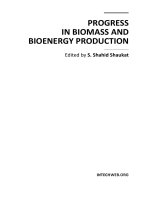
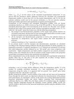
Fig. 14. Experimental and calculated radial temperature profiles 2 mm downstream of the
nozzle exit for 500 and 600 A with 27 and 32 slm of argon, partial characteristics method.
The so-called „new model“ stands for the present model, the „old model“ presents our
previous model with simplified plasma properties (see the text).
() ()
{}

=⋅ur McTr
,
where
()
{
}
cTr is the sonic velocity for the experimental temperature profile estimated from
the T&TWinner code (Pateyron, 2009). The drawback of this method is the assumption of
the constant Mach number over the nozzle radius. Nevertheless the existence of supersonic
Numerical Investigation of
Hybrid-Stabilized Argon-Water Electric Arc Used for Biomass Gasification

81
regime (i.e., the mean value of the Mach number over the nozzle exit higher than 1) using
this method was proved for 500 A and 40 slm of argon, as well as for 600 A for argon mass
flow rates higher than 27.5 slm. Similar results have been also reported in our previous work
(Jeništa et al., 2008).


Fig. 15. Average relative difference (see the text) between the calculated and experimental
radial temperature profiles, shown in %, at the axial position 2 mm downstream of the
nozzle exit, partial characteristics. The so-called „new model” stands for the present model,
exhibiting better agreement with experiments; the „old model” presents our previous model
with simplified plasma properties (see the text).
For more exact evaluation of velocity profiles we employed the so-called “integrated
approach”, i.e., exploitation of both experimental and numerical results: velocity profiles are
determined as a product of the Mach number profiles obtained from the present numerical
simulation and the sonic velocity based on the experimental temperature profiles. The
results for 300-600 A with 22.5 slm of argon for the partial characteristics method are
displayed in Fig. 16. Each graph contains four curves – velocity profiles based on the “new”

and “old” models (see above), the experimental velocity profile and the velocity profile
obtained by the “integrated approach” (the blue curves), we will call it “re-calculated”
velocity profile. It is clearly visible that agreement of such re-calculated experimental
velocity profiles with the numerical ones is much better than between original experiments
and calculation. High discrepancy between the “old” and “new” velocity profiles is also
apparent, especially for lower currents.
Fig. 17 presents the same type of plot as is presented in Fig. 15 but with the analogous
definition of the “average relative difference of velocity”
()
−−
=
Δ= ⋅ −

1
100
M
uiii
av re exp exp re exp
i
abs u u / u
M
,

Progress in Biomass and Bioenergy Production

82
where
−
i
re exp

u is the re-calculated velocity and
i
exp
u is the experimental velocity at the point
i , M is the number of available points at which the difference is being evaluated. It is again
evident that the present “new model” gives in most cases much lower relative difference
than the “old model” for all studied cases.


Fig. 16. Velocity profiles 2 mm downstream of the nozzle exit for 300 - 600 A with 22.5 slm of
argon. Calculation – partial characteristics model, re-calculated experimental profile is based
on the experimental temperature profile and calculated Mach number (see the text). The so-
called „new model“ stands for the present model, the „old model“ presents our previous
model with simplified plasma properties (see the text). The re-calculated velocity profiles
show better agreement with the experiment.
Numerical Investigation of
Hybrid-Stabilized Argon-Water Electric Arc Used for Biomass Gasification

83

Fig. 17. Average relative difference (see the text) between the calculated and re-calculated
(the experimental temperature profile and the calculated Mach number) radial velocity
profiles, shown in % at the axial position 2 mm downstream of the nozzle exit, partial
characteristics. The so-called „new model“ stands again for the present model and exhibits
better agreement with experiments than the „old model“.
3.3 Power losses from the arc
Energy balance, responsible for performance of the hybrid-stabilized argon-water electric
arc, is illustrated in the last set of figures. Fig. 18 (left) demonstrates the arc efficiency and
the power losses from the arc discharge as a function of current for 40 slm of argon. The arc
efficiency is defined here as

()
1 (power losses)/ UI
η
=− Δ⋅ with UΔ being the electric
potential drop in the discharge chamber and
I the current. The power losses from the arc
stand for the conduction power lost from the arc in the radial direction and the radiation
power leaving the discharge, which are considered to be the two principal processes
responsible for the power losses. The ratio of the power losses to the input power in the
discharge chamber
UIΔ⋅ is indicated as the power losses in a per cent scale: the maximum
difference of about 2-4 % between the net emission and partial characteristics methods is
obviously caused by the amount of radiation reabsorbed in colder arc regions, the partial
characteristics provides lower power losses. The arc efficiency is relatively high and ranges
between 77-82 % for the net emission model and 80-84 % for the partial characteristics. The
power losses slightly increases with increasing argon mass flow rate and with decreasing
current, see Fig. 18 (right).
Fig. 19 (left) displays the typical radial profiles of temperature, divergence of radiation flux
and radiation flux for 600 A and argon mass flow rate of 40 slm. Axial position is 4 cm from
the argon inlet nozzle, i.e., inside the discharge chamber. Temperature reaches 24 700 K at the
axis and declines to 773 K at the edge of the calculation domain. The radiation flux reaches
9.7
⋅ 10
6
W⋅ m
-2
at the arc edge with the maximum magnitude 3.1 ⋅ 10
7
W⋅ m
-2

at the radial
distance of 2.2 mm. The divergence of radiation flux becomes negative at the radial distance

Progress in Biomass and Bioenergy Production

84
over 2.6 mm, i.e., the radiation is being reabsorbed in this region. Despite the negative values
of the divergence of radiation flux in arc fringes are relatively small compared to the positive
ones in the axial region, the amount of reabsorbed radiation is 32.4% (understand: ratio of the
negative and positive contributions of the divergence of radiation flux, see below) because the
plasma volume increases with the third power of radius.


Fig. 18. Power losses and arc efficiency as functions of arc current for 40 slm of argon (left). The
arc efficiency (%) is defined as
()
()
1
p
ower losses / U I
η
=− Δ⋅ , where the power losses are due
to radiation and radial conduction. Power losses in % is the ratio
()
/
p
ower losses U IΔ⋅ , shown
also in dependence of current and argon mass flow rate (right).

Fig. 19. Radial profiles of temperature, divergence of radiation flux and radiation flux for 600
A and argon mass flow rate of 40 slm inside the discharge chamber at the axial position of 4
cm (left); partial characteristics. Reabsorption of radiation occurs at ~ 2.6 mm from the axis.
Reabsorption of radiation (right) for different currents and argon mass flow rates is defined as
the ratio of the negative to the positive contributions of the divergence of radiation flux - it
ranges between 30-45 % and slightly decreases for higher argon mass flow rates.
Numerical Investigation of
Hybrid-Stabilized Argon-Water Electric Arc Used for Biomass Gasification

85
Fig. 19 (right) shows the amount of reabsorbed radiation (%) in argon-water mixture plasma
within the arc discharge for the currents 300-600 A as a function of argon mass flow rate.
The negative and positive parts of the divergence of radiation flux are integrated through
the discharge volume. Reabsorption defined here is the ratio of the negative and positive
contributions of the divergence of radiation flux - it ranges between 31-45 % and increases
for lower contents of argon in the mixture.
Direct comparison of the amount of reabsorbed radiation with experiments is unavailable,
however the indirect sign of validity of our results is a very good agreement between the
experimental and calculated radial temperature profiles two millimeters downstream of the
outlet nozzle presented above.
4. Conclusions
The numerical model for an electric arc in the plasma torch with the so-called hybrid
stabilization, i.e., combined stabilization of arc by gas and water vortex, has been presented.
To study possible compressible phenomena in the plasma jet, calculations have been carried
out for the interval of currents 300-600 A and for relatively high argon mass flow rates
between 22.5 slm and 40 slm. The partial characteristics as well as the net emission
coefficients methods for radiation losses from the arc are employed. The results of the
present calculation can be summarized as follows:
a.
The numerical results proved that transition to supersonic regime starts around 400 A.

The supersonic structure with shock diamonds occurs in the central parts of the
discharge at the outlet region. The computed profiles of axial velocity, pressure and
temperature correspond to an under-expanded atmospheric-pressure plasma jet.
b.
The partial characteristics radiation model gives slightly lower temperatures but higher
outlet velocities and the Mach numbers compared to the net emission model.
c.
Reabsorption of radiation ranges between 31-45 %, it decreases with current and also
slightly decreases with argon mass flow rate. The arc efficiency reaches up to 77-84%, the
power losses from the arc due to radiation and radial conduction are between 16-24%.
d.
It was proved that simulations for laminar and turbulent regimes give nearly the same
results, so that the plasma flow can be considered to be laminar for the operating
conditions and a simplified discharge geometry studied in this paper.
e.
Comparison with available experimental data proved very good agreement for
temperature - the maximum relative difference between the calculated and
experimental temperature profiles is lower than 10% for the partial characteristics and
5% for the net emission radiation model used in the present calculation. Calculated
radial velocity profiles 2 mm downstream of the nozzle exit show good agreement with
the ones evaluated from the combination of calculation and experiment (integrated
approach). Agreement between the calculated radial velocity profiles and the profiles
analyzed purely from experimental data is worse. Evaluation of the Mach number from
the experimental data for 500 and 600 A give values higher than one close to the exit
nozzle, it thus proves the existence of the supersonic flow regime. The present
numerical model provides also better agreement with experiments than our previous
model based on the simplified transport, thermodynamic and radiation properties of
argon-water plasma mixture.
The existing numerical model will be further extended to study the effect of mixing of
plasma species within the hybrid arc discharge by the binary diffusion coefficients (Murphy,

1993, 2001) for three species - hydrogen, argon and oxygen.

Progress in Biomass and Bioenergy Production

86
5. Acknowledgments
J. Jeništa is grateful for financial support under the Fluid Science International COE Program
from the Institute of Fluid Science, Tohoku University, Sendai, Japan, and their computer
facilities. Financial support from the projects GA CR 205/11/2070 and M100430901 from the
Academy of Sciences AS CR, v.v.i., is gratefully acknowledged. Our appreciation goes also
to the Institute of Physics AS CR, v.v.i., for granting their computational resources
(Luna/Apollo grids)
. The access to the METACentrum supercomputing facilities provided
under the research intent MSM6383917201 is highly appreciated.

6. References
Bartlová, M. & Aubrecht, V. (2006). Photoabsorption of diatomic molecules. Czechoslovak
Journal of Physics
, Vol. 56, Suppl. B, (June 2006), pp. B632-B637, ISSN 0011-4626.
Březina, V.; Hrabovský, M.; Konrád M.; Kopecký, V. & Sember, V. (2001). New plasma
spraying torch with combined gas-liquid stabilization of arc,
Proceedings of 15
th

International Symposium on Plasma Chemistry
(ISPC 15), pp. 1021-1026, ISBN non-
applicable, Orleans, France, July 9-13, 2001.
Hrabovský, M.; Konrád M.; Kopecký, V. & Sember, V. (1997). Processes and properties of
electric arc stabilized by water vortex.
IEEE Transactions on Plasma Science, Vol. 25,

No.5, (October 1997), pp. 833-839, ISSN 0093-3813.
Hrabovský, M.; Kopecký, V. & Sember, V. (2003). Effect of Gas Properties on Characteristics
of Hybrid Gas/Water Plasma Spraying Torch,
Proceedings of 16-th International
Symposium on Plasma Chemistry (ISPC 16),
on CD-ROM, ISBN non-applicable,
Taormina, Italy, June 22-27, 2003.
Hrabovský, M.; Kopecký, V.; Sember, V.; Kavka, T.; Chumak, O. & Konrád, M. (2006).
Properties of hybrid water/gas DC arc plasma torch,
IEEE Transactions on Plasma
Science
, Vol. 34, No.4, (August 2006), pp. 1566-1575, ISSN 0093-3813.
Jameson, A. & Yoon, S. (1987). Lower-upper implicit schemes with multiple grids for the
Euler equations.
AIAA Journal, Vol. 25, No. 7, (July 1987), pp. 929-935, ISSN 0001-
1452, E-ISSN 1533-385X.
Jeništa, J.; Kopecký, V. & Hrabovský, M. (1999a). Effect of vortex motion of stabilizing liquid
wall on properties of arc in water plasma torch, In:
Heat and mass transfer under
plasma conditions
, editors: Fauchais, P.; Mullen, van der J. & Heberlein, J., pp. 64-71,
Annals of the New York Academy of Sciences, Vol. 891, ISBN 1-57331-234-7 (cloth),
ISBN 1-57331-235-5 (paper), ISSN 0077-8923, New York.
Jeništa, J. (1999b). Water-vortex stabilized electric arc: I. Numerical model
. Journal of Physics
D: Applied Physics
, Vol. 32, No. 21, (November 1999), pp. 2763-2776, ISSN 0022-3727
(print), ISSN 1361-6463 (online).
Jeništa, J. (2003a). Water-vortex stabilized electric arc: III. Radial energy transport,
determination of water-vapour-boundary and arc performance.

Journal of Physics D:
Applied Physics
, Vol. 36, No. 23, (December 2003), pp. 2995-3006, ISSN 0022-3727
(print), ISSN 1361-6463 (online).
Jeništa, J. (2003b). The effect of different regimes of operation on parameters of a water-
vortex stabilized electric arc.
Journal of High Temperature Material Processes, Vol. 7,
No. 1, (March 2003), pp. 11-16, ISSN 1093-3611 (print), ISSN 1940-4360 (online).
Numerical Investigation of
Hybrid-Stabilized Argon-Water Electric Arc Used for Biomass Gasification

87
Jeništa, J. (2004). Numerical modeling of hybrid stabilized electric arc with uniform mixing
of gases.
IEEE Transactions on Plasma Science, Vol. 32, No. 2, (April 2004), pp. 464-
472, ISSN 0093-3813.
Jeništa, J.; Bartlová, M. & Aubrecht, V. (2007). The impact of molecular radiation processes in
water plasma on performance of water-vortex and hybrid-stabilized electric arcs,
PPPS-2007 Proceedings of the 34th IEEE International Conference on Plasma Science and
The 16th IEEE International Pulsed Power Conference
, pp. 1429-1432, ISBN 1-4244-
0914-4, Albuquerque, New Mexico, USA, June 17-22, 2007.
Jeništa, J.; Takana, H.; Hrabovský, M. & Nishiyama, H. (2008). Numerical investigation of
supersonic hybrid argon-water-stabilized arc for biomass gasification.
IEEE
Transactions on Plasma Science
, Vol. 36, No. 4, (August 2008), pp.1060-1061, ISSN
0093-3813.
Jeništa, J.; Takana, H.; Nishiyama, H.; Bartlova, M.; Aubrecht, V. & Hrabovský, M. (2010).
Parametric study of hybrid argon-water stabilized arc under subsonic and

supersonic regimes.
Journal of High Temperature Material Processes, Vol. 14, No. 1-2,
(April 2010), pp. 63-76, ISSN 1093-3611 (print), ISSN 1940-4360 (online).
Kavka, T.; Chumak, O.; Sember, V. & Hrabovský, M. (2007). Processes in Gerdien arc
generated by hybrid gas-water torch,
Proceedings of XXVIII International Conference
on Phenomena in Ionized Gases (ICPIG 2007)
, pp. 1819-1822, ISBN 978-80-87026-01-4,
Prague, Czech Republic, July 15-20, 2007.
Kavka, T.; Maslani, A.; Chumak, O. & Hrabovský, M. (2008). Character of plasma flow at the
exit of DC arc gas-water torch,
Proceedings of 5-th International Conference on Flow
Dynamics
, pp. OS8-11, ISBN non-applicable, Sendai, Japan, November 17-19, 2008.
Křenek, P. & Něnička, V. (1984). Calculation of transport coefficients of a gas mixture in the
4-th approximation of Enskog-Chapman theory.
Acta Technica CSAV, Vol. 28, No. 4,
(1984), pp. 420-433, ISSN 0001-7043.
Křenek, P. (2008). Thermophysical properties of H
2
O–Ar plasmas at temperatures 400–
50,000 K and pressure 0.1 MPa.
Plasma Chemistry and Plasma Processes, Vol. 28, No.
1, (January 2008), pp. 107-122, ISSN 0272-4324.
Leer, van B. (1979). Towards the ultimate conservative difference scheme. V. A second-order
sequel to Godunov's method.
Journal of Computational Physics, Vol. 32, No. 1, (July
1979), pp. 101-136, ISSN 0021-9991.
Murphy, A. B. (1993). Diffusion in equilibrium mixtures of ionized gases,
Physical Review E,

Vol. 48, No. 5, (November 1993), pp. 3594-3603, ISSN 1539-3755 (print), ISSN 1550-
2376 (online).
Murphy, A. B. (2001). Thermal plasmas in gas mixtures,
Journal of Physics D: Applied Physics,
Vol. 34, No. 20-21, (October 2001), pp. R151–R173, ISSN 0022-3727 (print), ISSN
1361-6463 (online).
Patankar, S. V. (1980).
Numerical Heat Transfer and Fluid Flow, McGraw-Hill, ISBN 0-07-
048740-5, New York.
Pateyron, B. & Katsonis, C. (2009). T&TWinner, available from:
Roe, P. L. (1981). Approximate Riemann solvers, parameter vectors, and difference schemes.
Journal of Computational Physics, Vol. 43, No. 2, (October 1981), pp. 357-372, ISSN
0021-9991.
Van Oost, G.; Hrabovský, M.; Kopecký, V.; Konrád, M.; Hlína, M.; Kavka, T.; Chumak, O.;
Beeckman, E. & Verstraeten, J. (2006). Pyrolysis of waste using a hybrid argon-

Progress in Biomass and Bioenergy Production

88
water stabilized torch, Vacuum, Vol. 80, No. 11-12, (September 2006), pp. 1132-1137,
ISSN 0042-207X.
Van Oost, G.; Hrabovský, M.; Kopecký, V.; Konrád, M.; Hlína, M.; Kavka, T. (2008).
Pyrolysis/gasification of biomass for synthetic fuel production using a hybrid gas-
water stabilized plasma torch.
Vacuum, Vol. 83, No. 1, (September 2008), pp. 209-
212, ISSN 0042-207X.
Yoon, S. & Jameson, A. (1988). Lower-upper symmetric-Gauss-Seidel method for the Euler
and Navier-Stokes equations.
AIAA Journal, Vol. 26, No. 9, (September 1988), pp.
1025-1026, ISSN 0001-1452, E-ISSN 1533-385X.

Part 2
Biomass Production

5
A Simple Analytical Model
for Remote Assessment of the
Dynamics of Biomass Accumulation
Janis Abolins and Janis Gravitis
University of Latvia,
Latvian State Institute of Wood Chemistry,
Latvia
1. Introduction
Efficient means for assessment of the dynamics and the state of the stocks of renewable
assets such as wood biomass are important for sustainable supplies satisfying current needs.
So far attention has been paid mainly to the economic aspects of forest management while
ecological problems are rising with the expected transfer from fossil to renewable resources
supplies of which from forest being essential for traditional consumers of wood and for
emerging biorefineries. Production of biomass is more reliant on assets other than money
the land (territory) available and suitable for the purpose being the first in the number.
Studies of the ecological impacts (the “footprint”) of sustainable use of biomass as the source
of renewable energy encounter problems associated with the productivity of forest lands
assigned to provide a certain annual yield of wood required by current demand for primary
energy along with other needs.
Apart from a number of factors determining the productivity of forest stands, efficiency of
land-use concomitant with growing forest depends on the time and way of harvesting
(Thornley & Cannell, 2000). In the case of clear-cut felling the maximum yield of biomass
per unit area is reached at the time of maximum of the mean annual increment (Brack &
Wood, 1998; Mason, 2008). The current annual increment (rate of biomass accumulation by a
forest stand or rate of growth) culminates before the mean annual increment reaches its
peak value and there is a strong correlation between the maximums of the two measures.

Knowing the time of growth-rate maximum (inflection point on a logistic growth curve)
allows predicting the time of maximum yield (Brack & Wood, 1998). However, the growth-
rate maximum is not available from field measurements directly. Despite the progress in
development of sophisticated models simulating (Cournède, P. et al., 2009; Thürig, E. et al.,
2005; Welham et al., 2001) and predicting (Waring et al., 2010; Landsberg & Sands, 2010)
forest growth, there still remains, as mentioned by J. K. Vanclay, a strong demand for
models to explore harvesting and management options based on a few available parameters
without involving large amounts of data (Vanclay, 2010).
The self-consistent analytical model described here is an attempt to determine the best age
for harvesting wood biomass by providing a simple analytical growth function on the basis
of a few general assumptions linking the biomass accumulation with the canopy absorbing

Progress in Biomass and Bioenergy Production

92
the radiation energy necessary to drive photosynthesis. A number of reports on employing
remote sensing facilities (Baynes, 2004; Coops, et al., 1998; Lefsky et al., 2002; Richards &
Brack, 2004; Tomppo E. et al., 2002 ; Waring et al.,2010 ) strongly support the optimism with
regard to successful use of the techniques to detect the time of maximum yield of a stand
well in advance by monitoring the expanding canopy.
According to the grouping of models suggested by K. Johnsen et al. in an overview of
modeling approaches (Johnsen et al., 2001), the model described in this chapter belongs to
simplistic traditional growth and yield models. It differs from other models of this kind by
not incorporating mathematical representations of actual growth measurements over a
period of time. Derived from a few essential basic assumptions the analytical representation
rather provides the result that should be expected from measurements of growth under
“traditional” (idealized) conditions. The chosen general approach of modeling the biomass
production at the stand level allows obtaining compatible growth and yield equations
(Vanclay, 1994) of a single variable – the age. Like with many other theoretical constructions
the applicability of the model to reality is fairly accidental and restricted. However, since the

derived equations are in good agreement with the universal growth curves obtained from
measurements repeatedly confirmed and generally accepted as classic illustrations of
biomass dynamics (Brack & Wood, 1998; Mason et al., 2008), it seems to offer a good
approximation of the actual biomass accumulation by natural forest stands.
Equations representing the model are believed to reflect the simple assumptions made on
the basis of common knowledge about photosynthesis and observations in nature: biomass
is produced by biomass; the amount of produced biomass is proportional to the amount of
absorbed active radiation; the absorbed radiation is proportional to effective light-absorbing
area of the foliage (number and surface area of leaves) and limited by the ground area of
the forest stand (the area determining the available energy flow). Projection of the canopy
filling the ground area detectable by remote sensing is assumed to reflect dynamics and
status (the stage) of forest growth. The height of the stand is another growth parameter
accessible by remote sensing. Relationships of the latter with other measurable quantities
determining the yield of accumulated biomass are well studied (Vanclay, 2009) and can be
employed for remote assessment of the current annual increment and the state of forest
stands (Lefsky et al., 2002; Ranson et al., 1997; Tomppo et al., 2002). The model presented
hereafter has been developed to be aware of the current annual increment reaching the
maximum merely from the data of remote observation of the dynamics of forest stand
canopy while complemented by data of the average height would predict the yield.
2. General approach and basic equations
The analytical model offered to describe dynamics of the standing stock of wood biomass in
natural forests is based on the obvious relationship between the rate of growth (rate of
accumulation of biomass) y and the stock (amount of biomass) S stored in the forest stand
(Garcia, 2005):

() ()
St yt dt=⋅

(1)
By turning to common knowledge that biomass is produced by biomass the rate of

accumulation of new biomass in the first approximation can be assumed being proportional
to the amount of biomass already accumulated:

A Simple Analytical Model for Remote Assessment of the Dynamics of Biomass Accumulation

93

dS
y
aS
dt
==
(2)
where
a is a constant of the reciprocal time dimension and t is time. Rewriting the right-side
equation of (2) in the form:

dS
adt
S
=
, (3)
and integrating it provides ln
Sat= and exponential growth of the stock of biomass:

at
Sconste=⋅, (4)
which is unrealistic in the long run because of finite resources of nutrients and other limiting
factors not taken into account in Eq. (2). The problem can be solved by setting an asymptotic
limit to growth:

()
()
1
at
St S e
−
∞
=⋅− . (5)
The rate of biomass accumulation
y, Eq. (2), usually referred to as the current annual
increment of stock measured by volume of wood mass per unit area (
m
3
/ha) (Brack & Wood,
1998) is not directly determined by the accumulated biomass stock. The uptake of CO
2
and
photosynthesis of biomass rather depends on the total surface area of leaves determining the
amount of absorbed radiation. The number of leaves and hence the light-absorbing area
depend on the biomass accumulated by individual trees and the forest stand as a whole. The
actual amount of the absorbed radiation that ultimately determines the rate of
photosynthesis (and the annual increment) per unit area (a
hectare) of a particular forest
stand is limited regardless of the total surface area of leaves. So the concept of light-
absorbing area should refer to the effective absorbing area limited by the particular area unit
selected. It should be noticed here that further considerations are relevant to statistically
significant numbers of individual trees and, consequently, to area units of stands
comparable to hectare.
It seems to be reasonable to assume that accumulation of biomass in a forest stand

occupying a large enough land area follows the same law as the rate at which the light-
absorbing area (the canopy) of the growing stand expands with time. As noticed, the
number and total surface area of leaves absorbing radiation is proportional to the
accumulated biomass approaching some asymptotic limit
L
∞
of its own. However, the rate
of expansion of the effective absorbing area also depends on the proportion of the free,
unoccupied space available for expansion to intercept the radiation. Supposing the total
light-absorbing area
L as function of time being described by equation similar to Eq. (5):

()
()
1
at
Lt L e
−
∞
=−
, (6)
the rate of expansion of the light-absorbing area expressed as:

()
dL
const L L L
dt
∞
=⋅−⋅ (7)

Progress in Biomass and Bioenergy Production

94
can be written in the form:

()() ()
2
11 1
at at at at
dL
const L L e L e const L e e
dt
−− −−
∞∞ ∞ ∞

=⋅−⋅− ⋅−=⋅⋅⋅−

. (8)
Dimension of the constant in Eq. (8) is the reciprocal of the product of area and time. Since
area
L
∞
also is constant it can be omitted for further convenience to focus attention on the
time-dependent part of Eq. (8).
Assuming that the rate of biomass accumulation follows the rate of expansion of the light-
absorbing area it can be described by equation similar to Eq. (8):

()
1
at at

dS
const e e
dt
−−
=⋅−⋅
, (9)
where the value of the constant factor (dimension of which here is the dimension of current
increment) can be chosen to satisfy some selected normalizing condition, as will be done
further.
The time-dependent part of Eq. (9) has a maximum at time
t
m
satisfying condition:

210
at
e
−
−= (10)
Wherefrom

ln 2
m
at = (11)
Exponent
a determining the rate of growth in real time depends on the particular species
and a number of other factors such as insolation and availability of water and nutrients at
the site and has to be found from field measurements. However, existence of the maximum
on the curve of the rate of growth (the curve of current annual increment often referred to as
the growth curve) allows normalizing the time scale with respect to the time at which the

maximum is reached. It is done by introducing dimensionless time variable

ln 2
at
x =
, (12)
or substituting
at with x·ln2 in Eq. (9), or just writing x instead of t and putting a = ln2. The
current annual increment is normalized by choosing the constant factor to satisfy
condition:

()
11 1
11 1
22 4
m
yyx const const

===⋅−⋅=⋅=


. (13)
The normalized rate of biomass accumulation expressed by current annual increment in
time scale
x normalized with respect to the time when it reaches its maximum now is
presented by Eq. (9) where
t is substituted by variable x:

()
()

41
ax ax
dS
y
xee
dx
−−
≡=⋅− ⋅
(14)
where
a = ln2. Function y(x) is shown in Fig. 1 (a).

A Simple Analytical Model for Remote Assessment of the Dynamics of Biomass Accumulation

95

Fig. 1. a – rate of accumulation (current annual increment) of biomass
y(x) normalized with
respect to its maximum value presented by Eq. (14) and b – stock normalized with respect to
its asymptotic limit presented by Eq. (17) as functions of normalized time variable
x.
Returning to Eq. (1) the biomass stored by time x = x
c
is expressed by definite integral:

()
()
0
c
x

c
Sx yxdx=

. (15)
Substituting
y(x) from Eq. (14) into Eq. (15) and calculating the integral the stock S is
presented as function of age explicitly:
()
()
2
2
000
0
41 4 4 4
2
c
ccc
x
xxx
ax ax
ax ax ax ax
c
ee
S x e e dx e dx e dx
aa
−−
−− − −

=−⋅ = − =−+ =







()()
2
2
2
0
22 2
2211
22 2
c
cc c
x
ax ax ax
ax ax
ee e e e
aa a
−− −
−−

=⋅ − =⋅ − +=⋅−

(16)
By normalizing the stock choosing its asymptotic limit as the normalized unit S
∞
= 1 the
result of transformations in Eq. (16) can be summarized as

()
()()
22
2
11
2
cc
ax ax
c
Sx e S e
a
−−
∞
=⋅− = −
(17)
where, as previously in Eq. (14), a = ln2. Function (17) in the normalized time scale is
presented in Fig. 1 (b).
3. Mean annual increment and productivity
The mean annual increment of a forest stand is an essential factor illustrating the overall
productivity of the stand at a given age and is expressed by the ratio of stock to age of the
stand (Brack & Wood, 1998). The stock being presented by Eq. (16) the mean annual
increment Z is calculated in units of the current annual increment from
S
(
x
)
y(x)
time time
a b

Progress in Biomass and Bioenergy Production

96

()
()
2
1
2
ax
e
Zx
ax
−
−
=⋅ (18)
where a = ln2. Function Z(x) shown in Fig. 2 has a maximum at x satisfying condition:

ln 2
2ln2
x
e
x
= (19)
obtained from putting derivative of function (18) equal to zero. The value of x ≈ 1.81
satisfying Eq.(19) is found from graphical solution of the equation (Fig. 3).


Fig. 2. Mean annual increment Eq. (18) as function of the normalized time variable x.

Fig. 3. Graphical solution of Eq. (19) determining position of the maximum of mean annual
increment on the axis of the normalized time coordinate x.
Z
(
x
)
x

A Simple Analytical Model for Remote Assessment of the Dynamics of Biomass Accumulation

97
In Fig. 4 the current annual increment (rate of biomass accumulation) and the mean annual
increment are presented together wherefrom the mean annual increment is seen to reach the
maximum value (equal to ≈ 0.8 of the peak value of current annual increment) at cross-point
of the two curves.


Fig. 4. Current (curve 1, Eq. 14) and mean (curve 2, Eq. 18) annual increments of biomass as
functions of time x normalized with respect to the time of the growth-rate maximum chosen
as the unit time interval. The mean annual increment (curve 2) is presented in the same scale
as the current annual increment. The maximum of curve 2 is reached at the cross-point of
the two curves at x ≈ 1.81.
The reciprocal of the mean annual increment is a parameter characterizing the size of
plantation for sustainable supply of biomass. The total area of a plantation for sustainable
annual supply comprised of equal lots of stands of ages in sequence from one year to the
cutting age is directly proportional to cutting age x
c
and inversely proportional to the stock

at cutting age S(x
c
):

()
()
c
c
c
x
Aconst constfx
Sx
=⋅ =⋅
. (20)
The constant is equal to the required annual yield of biomass; function
f(x
c
) defined as

()
()
c
c
c
x
fx
Sx
≡
(21)
is the reciprocal of the mean annual increment at cutting age.

At point
x ≈ 1.81 where the mean annual increment reaches maximum its reciprocal –
function
f(x) has the minimum. If B
s
is the demanded sustainable annual yield of biomass,
S(x
c
) – the stock of biomass accumulated in the forest stand by the cutting age, and A
o
– the
area of the forest to be felled annually to satisfy the demand
,
then B
s
= S(x
c
)·A
o
and the total

Progress in Biomass and Bioenergy Production

98
area of the plantation – A = x
c
·A
o
. From here the yield per unit area of the whole plantation
is found being proportional to the mean annual increment reaching the maximum at

x ≈ 1.8:

() ()
cocc
s
co c
Sx A S x
B
AxA x
⋅
==
⋅
. (22)
As follows from Eq. (22), felling the forest at age corresponding to 1.8 units of the
normalized time scale provides the maximum yield per unit area of a particular stand and
hence of the whole plantation. In other words, the maximum productivity of land area
under a forest is achieved when felling at the time of the mean annual increment peak.
4. Validation of the model
Neither the value of the current annual increment at maximum, nor the real time when a
forest stand reaches the maximum is known
a priori. Both parameters depend on the species
and conditions represented by the quality class of the site and have to be determined by
field measurements. However, the field measurements do not provide these quantities
directly. They have to be found from periodic mean annual increments available from field
measurements.
The growth-rate function given by Eq. (14) cannot be used directly to compare the model
equation with experimental growth-rate data. For that purpose a different exponential
equation can be employed containing variable parameters related to the quantities not
measurable directly. The values of the variable parameters providing the best fit of the
measured annual increments with the equation are chosen to evaluate the unknown

quantities. A rather abundant database available for natural grey alder (
Alnus incana) stands
of up to 50 years old (Daugavietis, 2006) presents a good opportunity to test the model.

The 5-year mean annual increments available from field measurements (Daugavietis, 2006)
are a good approximation for the current annual increment value at mid-time of the
respective 5-year period (Fig. 5, a). By choosing a function of the type

() ( ) ()
tt
aa
y
tckte kbte
−−
=+ ⋅ = +⋅ (23)
to describe the current annual increment it is possible to assign physical sense to variable
parameters
a and c and find the maximum value of the current annual increment and
position of the maximum on the real-time axis by best fit of function (23) to the data from
experimentally measured periodic mean increments. Under condition of taking coefficient
k
(of dimension
y/t) equal to 1 function (23) has its maximum at time

m
c
ta ab
k
=− =−
. (24)

It should be noticed here that dimension of constant
a in Eq. (23) is time, which is different
from the constant
a used in Eq. (2) with dimension of reciprocal time (frequency). The
reason of choosing a different dimension of constant
a in Eq. (23) is seen from Eq. (24).
By varying parameters
a, b, and the maximum value of the current annual increment y
m
(not
available from any direct measurement) function (23) is varied for best fit to the set of
experimental data normalized with respect to
y
m
.

A Simple Analytical Model for Remote Assessment of the Dynamics of Biomass Accumulation

99
The values of increments calculated from Eq. (23) coincide with the set of experimental data
(Daugavietis, 2006) (Fig. 5) within standard deviation of 2.5 % of the maximum value, the
correlation between the sets of calculated and experimental data being better than 0.99.
The normalized time scale is introduced by choosing variable x to satisfy condition

m
tt
x
tab
==
−

. (24)
By substituting the normalized time variable
x for real time t in Eq. (23) the current annual
increment is presented as

() ( )
ab
x
a
yx b a b x e
−
−⋅
=  +−⋅ ⋅

. (25)
By defining new constant parameters
ab
a
α
−
=
and
b
ab
β
=
−
Eq. (25) is rewritten as:

() ( )( )

x
y
xab xe
α
β
−
=−⋅ +⋅
. (26)
Normalizing function (26) with respect to y
m
= (a – b)·(β + 1)·exp(-α) and taking into account
that
1
bab a
ab ab
β
+−
+= =
−−
provide

() ( )
x
y
xe xe
αα
αβ
−
=⋅ ⋅ + ⋅ . (27)
By substituting

y(x) from Eq. (27) in Eq. (15) and calculating the integral the stock
normalized to
()
()
2
aab
S
ab
∞
⋅+
=
−
as function of cutting age is expressed by:

()
11
c
x
cc
ab
Sx x e
ab
α
−
−

=− + ⋅ ⋅

+


. (28)
The mean annual increment

()
()
1
11
x
Sx
ab
yx x e
xx ab
α
−

−

==⋅−+⋅⋅



+



(29)
reaches maximum under condition

()
exp 1 1

ab
xx x
ab
αα
−

−⋅+ =

+

(30)
providing
x
m
≈ 1.77 corresponding to optimum cutting age of x
c
= 1.8 or 18 years in case of
grey alder.
After finding the age of the maximum of current annual increment, the set of
experimental points (Fig. 5, a) can be put on the normalized time scale
x and compared
with function (14) as shown in Fig. 5, b. The variation of the value of growth-rate
maximum at this point is still available for adjustment to improve the fit between

Progress in Biomass and Bioenergy Production

100
experimental data and Eq. (14). The curves presented by Eqs. (14) and (27) with best fit
parameter values are practically identical within the normalized time interval 0.5 ≤ x ≤ 2.5.
Because of a nonzero initial growth-rate Eq. (27) provides higher values on the rise while

lower at later time on the decline.


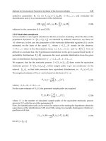
Fig. 5. a – current annual increments of grey alder stand calculated from measured 5-year
periodic mean values with age (Daugavietis, 2006), in units of
m
3
per ha per annum; b – best
fit of Eq. (14) (solid curve) to experimental data (circles) normalized against the growth-rate
maximum in the time scale of normalized age.
5. Rate of growth as function of light-absorbing area
Equation (9) describing the rate of biomass accumulation derived from Eq. (7) in section 1 is
based on the assumption that dynamics of current annual increment follows dynamics of
the expansion of light-absorbing area of the canopy. Returning to Eq. (7) it can be assumed
to describe the relationship between the normalized rate of growth (
y) and the normalized
light-absorbing area (
L):

() ( )
41
y
LLL=⋅ −
(31)
shown in Fig. 6.
It has to be noticed that the pace at which the biomass is stored is not necessarily equal to
the pace at which the light-absorbing area increases. The uptake of biomass (photosynthesis)
depending on the effective light-absorbing area obviously should follow with some delay,
which means that the normalized (intrinsic or specific) time scale of the equation derived
from Eq. (8) to describe the rate of expansion of the light-absorbing area:

()
41
ax ax
dL
ee
dx
−−
=− ⋅
, (a = ln2) (32)
is different from that of Eq. (14) describing the rate of biomass accumulation.
m
3
ha
-1
a
-1
annual increment

time
a b
age

A Simple Analytical Model for Remote Assessment of the Dynamics of Biomass Accumulation

101

Fig. 6. Rate of biomass accumulation y as a function of the light-absorbing area L, Eq. (31).
Relationship between the units of the two normalized time variables – x
b

describing the
current annual increment (rate of biomass accumulation) and x
a
describing the rate of
expansion of the light-absorbing area can be concluded from knowing that maximum of the
current annual increment is reached at L/L
∞
= 0.5 when x
b
= 1. In units of time scale x
a
the
light-absorbing area L is expressed by integrating Eq. (32) the result of which is similar to
Eq. (17):

()
()
2
1
a
ax
a
Lx L e
−
∞
=− (33)
where L is normalized in the same way as stock by taking the asymptotic limit L
∞
equal to 1.
The “age” x

a
at which the normalized light-absorbing area reaches the value 0.5, as follows
from Eq. (33), satisfies equation:

2
1
2
a
ax
e
−
−= (34)
wherefrom, remembering that a = ln2, the time in units of scale x
a
corresponding to unit time
of scale x
b
= 1 is found being equal to

2
ln 1
2
1.77
ln 2
a
x

−−




=≅. (35)
It means that a unit of the normalized time scale of the rate of expansion of the light-
absorbing area is about 0.56 of the unit of the normalized time scale describing the rate of
biomass accumulation. The units of the two normalized time scales presented in Fig. 7 are
approximately equated by
L
L
∞
y
(
L
)

Progress in Biomass and Bioenergy Production

102
1.77
ba
xx≅ . (36)
As seen from Fig. 7, expansion of the light-absorbing area of the canopy (curve 1) proceeds
ahead of the rate of biomass accumulation (curve 2) complying with the assumption that
higher rates of the increase of the surface area (and the number) of leaves require a greater
proportion of the gross product of photosynthesis lost after seasonal vegetation.
The size of the effective light-absorbing area expressed by the ratio to its asymptotic limit is
presented in Fig. 7 on the lower time axis. The maximum rate of expansion dL/dx is reached
at x = x
b
≈ 0.56 (x
a

= 1) when L = 0.25L
∞
while the current annual increment reaches the
maximum at x = x
b
= 1 when L = 0.5L
∞
. By the time x = x
b
≈ 1.81 when the mean annual
increment reaches its maximum the effective light-absorbing area is equal to approximately
0.8 L
∞
. The current annual increment of biomass in the stand is maintained over 0.8 of the
maximum value within the range of light-absorbing area between 0.28 and 0.8 of L
∞
.


Fig. 7. Rate of expansion of the light-absorbing area (1), current annual increment (2), and
the light-absorbing area (3) in time-scale x = x
b
normalized to the time of the current annual
increment maximum. The lower axis shows the size of the light-absorbing area reached at
the respective point on the time axis.
The basic components of the model – equations presenting current and mean annual
increments, stock, and the rate of expansion of the light-absorbing area as functions of age
expressed in the intrinsic time units are summarized in Fig. 8.
6. Conceptual remarks
The analytical expressions comprising the model are derived from rather general principles

of biomass production by photosynthesis in living stands without taking into account
L
L
∞

A Simple Analytical Model for Remote Assessment of the Dynamics of Biomass Accumulation

103
factors affecting forest growth other than the effective light-absorbing area of the canopy.
However, since dynamics of the latter is strongly dependent on availability of nutrients,
water, and some other crucial factors, the model reflects the cumulative effect of all of them
through the relationship between the rate of growth and the capacity to capture the active
radiation. Therefore, monitoring the canopy dynamics can provide reliable information for
conclusions about that capacity and the expected end product of photosynthesis.
Determining the best time for harvesting by observing expansion of the canopy from
satellites is one of attractive practical applications of the model for management of even-age
stands in concert with remote sensing. Even though the canopy projection measureable by
remote sensing instruments is not quite equal either to the light-absorbing area or the leaf
area index, the correlation between the three is strong enough to make corrections necessary
for detecting the time (age) of growth-rate maximum from remote observations of the
dynamics of canopy expansion.


Fig. 8. Dynamics of the light-absorbing area (1), Eq. (7), the rate of production of above-
ground biomass (2), Eq. (14), mean annual increment (3), Eq. (18), and the yield (4), Eq. (17),
as functions of the intrinsic time provided by the rate of growth of a forest stand. The
effective light-absorbing area as the ratio to its maximum value L/L
∞
, Eq. (33), is presented
by the lower abscissa. Note the inflection point of curve 4 being reached before 0.25 S

∞
; at
the time of maximum productivity S
@ 0.5 S
∞
.
The obtained analytical expression, Eq. (17), for accumulated biomass of a stand as function
of age is a particular case of the well-known Richards growth equation (Zeide, 2004):
L
L
∞