Progress in Biomass and Bioenergy Production Part 5 potx

Assessment of Forest Aboveground Biomass Stocks and
Dynamics with Inventory Data, Remotely Sensed Imagery and Geostatistics

109
schemes for image data and ground data; to increase the accuracy in which remotely sensed
data can be used to classify land cover; or to estimate continuous variables. Geostatistical
models are reported in numerous textbooks (e.g. Isaaks & Srivastava, 1989; Cressie 1993;
Goovaerts, 1997; Deutsch & Journel, 1998; Webster & Oliver, 2007; Hengl, 2009; Sen, 2009) such
as Kriging (plain geostatistics); environmental correlation (e.g. regression-based); Bayesian-
based models (e.g. Bayesian Maximum Entropy) and hybrid models (e.g. regression-kriging).
Despite Regression-kriging (RK) is being implemented in several fields, as soil science, few
studies explored this approach to spatially predict AGB with remotely sensed data as
auxiliary predictor. Hence, this research makes use of RK and remote sensing data to
analyse if spatial AGB predictions could be improved.
This research presents two case studies in order to explore the techniques of remote sensing
and geostatistics for mapping the AGB and NPP. The first, aims to compare three approaches
to estimate Pinus pinaster AGB, by means of remotely sensed imagery, field inventory data and
geostatistical modeling. The second aims to analyse if NPP of Eucalyptus globulus and Pinus
pinaster species can easily and accurately be estimated using remotely sensed data.
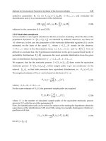
2. Case study I – Aboveground biomass prediction by means of remotely
sensed imagery, field inventory data and geostatistical modeling
2.1 Study area
This study was carry out in Portugal (Continental), extending from the latitudes of 36º 57’
23” and 42º 09’ 15”N and the longitudes of 09º 30’ 40” and 06º 10’ 45” W (Figure 1). This area


Fig. 1. Study area location

Progress in Biomass and Bioenergy Production

110

includes two distinctive bioclimatic regions: a Mediterranean bioclimate in everywhere
except a small area in the North with a temperate bioclimate. With four distinct weather
seasons, the average annual temperatures range from about 7 °C in the highlands of the
interior north and center and about 18 ° C in the south coast. Average annual precipitation is
more than 3000 mm at the north and less than 600 mm at the south.
Due to a 20 years of severe wild fires during summer time, and intense people movement
from rural areas to sea side cities or county capital, forestry landscape changed from large
trees’ stands interspersed by agricultural lands, to a fragmented landscape. The land cover is
fragmented with small amount of suitable soils for agriculture and the main areas occupied
by forest spaces. Forest activity is a direct source of income for a vast forest products
industry, which employs a significant part of the population.
2.2 Methods and data
2.2.1 GIS and field data
In a first stage a GIS project (ArcGis 9.x), was created in order to identify Pinus pinaster pure
stands, over a Portuguese Corine Land Cover Map (CLC06, IGP, 2010). In a second stage,
GIS project database was updated with the dendrometric data collected during Portuguese
National Forestry Inventory (AFN, 2006), in order to derive AGB allometric equations, with
Vegetation Indices values as independent variable. A total of 328 field plots of pure pine
stands were used. The inventory dataset was further used in spatial prediction analysis, to
create continuous AGB maps for the study area.
2.2.2 Biomass estimation from the forest inventory dataset
In order to calculate the biomass exclusively from the forest inventory, the biomass values
measured in each field plot were spatially assigned to the pine stands land cover map
polygons. In the cases where multiple plots were coincident with the same polygon,
weighted averages were calculated proportionally to the area of occupation in that polygon.
2.2.3 Remote sensing imagery
In this research we used the Global MODIS vegetation indices dataset (h17v04 and h17v05)
from the Moderate Resolution Imaging Spectroradiometer (MODIS) from 29 August 2006:
(MOD13Q1.A2006241.h17v04.005.2008105184154.hdf; and
MOD13Q1.A2006241.h17v05.005.2008105154543.hdf), freely available from the US Geological

Survey (USGS) Earth Resources Observation and Science (EROS) Center. The Global
MOD13Q1 data includes the MODIS Normalized Difference Vegetation Index (NDVI) and a
new Enhanced Vegetation Index (EVI) provided every 16 days at 250-meter spatial resolution
as a gridded level-3 product in the Sinusoidal projection.
( />day_l3_global_250m/mod13q1).
MODIS data was projected to the same Portuguese coordinate system (Hayford-Gauss,
Datum of Lisbon with false origin) used in the GIS project.
2.2.4 Direct Radiometric Relationships (DRR)
Using GIS tools, field inventory dataset was updated with information from MODIS
images. The spectral information extracted (NDVI and EVI) was then used as independent
variables for developing regression models. Linear, logarithmic, exponential, power,
Assessment of Forest Aboveground Biomass Stocks and
Dynamics with Inventory Data, Remotely Sensed Imagery and Geostatistics

111
and second-order polynomial functions were tested on data relationship analysis.
The best model achieved was then applied to the imagery data, and the predicted
aboveground biomass map was produced. In some pixels where Vegetation index
values were very low, the biomass values predicted by the regression equations were
negative, so these pixels were removed, because in reality negative biomass values are not
possible.
2.2.5 Geostatistical modeling
Regression-kriging (RK) (Odeh et al., 1994, 1995) is a hybrid method that involves either a
simple or multiple-linear regression model (or a variant of the generalized linear model and
regression trees) between the target variable and ancillary variables, calculating residuals of
the regression, and combining them with kriging. Different types or variant of this process,
but with similar procedures, can be found in literature (Ahmed & De Marsily, 1987; Knotters
et al.; 1995; Goovaerts; 1999; Hengl et al.; 2004, 2007), which can cause confusion in the
computational process.
In the process of RK the predictions

()
0
()
ˆ
rk S
z
are combined from two parts; one is the
estimate
0
ˆ
()ms
obtained by regressing the primary variable on the k auxiliary variables
k0
q(s) and
00
q(s) 1 = ; the second part is the residual estimated from kriging
()
0
()
ˆ
S
e
. RK is
estimated as follows (Eqs. 1 and 2):

() () ()
000
ˆˆˆ
rk
zs ms es=+

(1)

() () ()()
000
01
ˆ
ˆ
vn
rk k k i i
ki
zs qs ws es
β
==
=⋅ + ⋅

(2)
where
ˆ
k
β
are estimated drift model coefficients (
0
ˆ
β
is the estimated intercept), optimally
estimated from the sample by some fitting method, e.g. ordinary least squares (OLS) or,
optimally, using generalized least squares (GLS), to take the spatial correlation between
individual observations into account (Cressie, 1993);
i
w are kriging weights determined by the

spatial dependence structure of the residual and
()
i
es are the regression residuals at location s
i
.
RK was performed using the GSTAT package in IDRISI software (Eastman, 2006) both to
automatically fit the variograms of residuals and to produce final predictions (Pebesma,
2001 and 2004). The first stage of geostatistical modeling consists in computing the
experimental variograms, or semivariogram, using the classical formula (Eq. 3):

[]
2
()
1
1
ˆ
() ( ) ( )
2()
Nh
ii
i
hzxzxh
Nh
γ
=
=−+

(3)
where

ˆ
()h
γ
is the semivariance for distance h, N(h) the number of pairs for a certain distance
and direction of
h units, while z(xi) and Z(x
i
+ h) are measurements at locations x
i
and x
i
+ h,
respectively.
Semivariogram gives a measure of spatial correlation of the attribute in analysis. The
semivariogram is a discrete function of variogram values at all considered lags (e.g. Curran
1988; Isaaks & Srivastava 1989). Typically, the semivariance values exhibit an ascending

Progress in Biomass and Bioenergy Production

112
behaviour near the origin of the variogram and they usually level off at larger distances (the
sill of the variogram). The semivariance value at distances close to zero is called the nugget
effect. The distance at which the semivariance levels off is the range of the variogram and
represents the separation distance at which two samples can be considered to be spatially
independent.
For fitting the experimental variograms we tested the exponential, the gaussian and the
spherical models, using iterative reweighted least squares estimation (WLS, Cressie, 1993).
Finally, RK was carried out according to the methodology described in http://spatial-
analyst.net. The EVI image was used as predictor (auxiliary map) in RK. GSTAT produces
the predictions and variance map, which is the estimate of the uncertainty of the prediction

model, i.e. precision of prediction.
2.2.6 Validation of the predicted maps
The validation and comparison of the predicted AGB maps were made by examining the
discrepancies between the known data and the predicted data. The dataset was, prior to
estimates, divided randomly into two sets: the prediction set (276 plots) and the
validation set (52 plots). According to Webster & Oliver (1992), to estimate a variogram
225 observations are usually reliable. The prediction approaches were evaluated by
comparing the basic statistics of predicted AGB maps (e.g., mean and standard deviation)
and the difference between the known data and the predicted data were examined using
the mean error, or bias mean error (ME), the mean absolute error (MAE), standard
deviation (SD) and the root mean squared error (RMSE), which measures the accuracy of
predictions, as described in Eqs. (4-7).

()
2
1
1
1
N
i
i
SD e e
N
=
=−
−

(4)

()

1
1
ˆ
N
ii
i
M
Eee
N
=
=−

(5)

1
1
ˆ
N
ii
i
M
AE e e
N
=
=−

(6)

()
2

1
1
ˆ
N
ii
i
RMSE e e
N
=
=−

(7)
where: N is the number of values in the dataset, ê
i
is the estimated biomass, e
i
is the
biomass values measured on the validation plots and
e is the mean of biomass values of
the sample.
2.3 Results and discussion
2.3.1 Pinus pinaster stands characteristics
The descriptive statistics of pine stands data are presented in Table 1, where: N is the
number of trees; t is the forestry stand age; h
dom
is the dominant height; dbh
dom
is the
dominant diameter at breast height; SI is the site index; BA is the basal area; V is the stand
volume and AGB is the biomass in the sample plot.

Assessment of Forest Aboveground Biomass Stocks and
Dynamics with Inventory Data, Remotely Sensed Imagery and Geostatistics

113
The pine stands are highly heterogeneous with ages ranging from 8 to 110 years old and the
biomass per hectare ranging from 0.9 to 136.1 ton ha
-1
. The values of Biomass present a
normal distribution with mean m = 52.12 ton ha
-1
and standard deviation σ = 32.32 ton ha
-1

(Figure 2).


Pine stands plots

N t h
dom
dbh
dom
SI BA V AGB
(trees ha
-1
) (year) (m) (cm) (m) (m
2
ha
-1
)(m

3
ha
-1
) (ton ha
-1
)
Mean 566 31 13.4 25.3 11.8 14.39 99.46 52.12
Min 20 8 4.6 8.9 0.0 0.41 1.37 0.85
Max 2219 110 36.5 59.0 69.0 38.34 259.03 136.09
SD 405.2 15.9 4.0 8.0 11.5 7.64 61.86 32.32
Table 1. Descriptive statistics of data measured in the forest inventory dataset


Fig. 2. Histogram of the distribution of the AGB (ton ha
-1
) in the forest inventory dataset
2.3.2 Aboveground biomass estimation from the inventory dataset
The estimates based in the inventory dataset were achieved by assigning the 328 field plot
biomass values (weighted by each polygon area) into all the polygons of the pine cover
class. After the global calculation, the dataset used for training (276 plots) was used to make
a first validation of this approach. Hence, a regression was established between the biomass
values, measured in the field plots, and the forest inventory polygon data. In Figure 3 it is
presented the positive relationship between the measured and the predicted data with a
coefficient of determination (R
2
) of 0.71.

Progress in Biomass and Bioenergy Production

114

R
2
= 0.71
0.0
20.0
40.0
60.0
80.0
100.0
120.0
140.0
0.0 20.0 40.0 60.0 80.0 100.0 120.0 140.0
Field Plots Biomass (ton ha
-1
)
Forest Inventory Polygon Biomass (ton ha
-1
)

Fig. 3. Relationship between the biomass data measured in field plots and the predicted data
extracted in the polygons of land cover map
2.3.3 Aboveground biomass estimation from DRR
After performing correlation analyses, between AGB and Vegetation indices, several
regression models were developed using stand-wise forest inventory data and the MODIS
vegetation indices (NDVI and EVI) as predictors.


Fig. 4. MODIS image showing the effect of pixels (250m) in the edge of polygons
Assessment of Forest Aboveground Biomass Stocks and
Dynamics with Inventory Data, Remotely Sensed Imagery and Geostatistics

115
The best correlation was obtained with EVI as independent variable as (Eq. 8):
AGB = 322.4(EVI) - 39.933 (R
2
= 0.32) (8)
The AGB was then estimated for the entire study area. The low correlation achieved is
explained, in part, by the heterogeneity of pine stands and the high effect of mixed pixels
(Burcsu et al., 2001) in coarse resolution MODIS data (250 m).
As it can be seen in Figure 4, the reflectance value recorded in the boundary pixels of the
polygons limits is not pure, they record both pine stands, and the neighbouring land cover
classes reflectance values.
2.3.4 Aboveground biomass estimation from geostatistical methods
To spatially estimate the AGB by geostatistical approach, the first step consisted in the
modeling and analysis of the experimental semivariograms (Eq. 3). The directional
semivariograms of the residuals showed anisotropy at 38.6º, so at this direction were fitted
Exponential, Gaussian and Spherical models. Based on experimentation, the exponential
variogram model was fitted better (nugget of 703.75 and a partial sill of 390.17 reaching its
limiting value at the range of 43,9Km) to the calculated biomass pine stands data (Figure 5).
The present data showed a low spatial autocorrelation. The high nugget effect, visible in the
figure, which under ideal circumstances should be zero, suggests that there is a significant
amount of measurement error present in the data, possibly due to the short scale variation.

Distance, h 10
-4
γ 10
-3
0 0.58 1.15 1.73 2.31 2.88 3.46 4.04 4.6
2
0.3

0.6
0.9
1.2
1.5
Dis tanc e, h 10
-4
C 10
-3
0 0.581.151.732.312.883.464.044.62
-0.51
-0.21
0.08
0.38
0.68
0.97

Fig. 5. Directional experimental semivariogram (38.6º) with the exponential model fitted (a)
and covariance (b)
2.3.5 Validation and comparison of the aboveground biomass estimation approaches
The validation of the AGB estimation approaches was made by comparing the calculated
basic statistics (Table 2) in the 52 validation random samples. Training and validation sets
were compared, by means of a Student's t test (t = 0.882 ns), in order to check if they
provided unbiased sub-sets of the original data.
As expected, the Inventory Polygons method produced the best statists. The mean error
(ME), which should ideally be zero if the prediction is unbiased, shows a bias in the three
approaches, being lower in the Inventory polygons method, and higher in the DRR method.
The analysis of the root mean squared errors (RMSE), shows that Inventory Polygons
present the lower discrepancies in the estimations (RMSE=33.53%), and RK achieve
estimations under lower errors (RMSE=51.95%) than the DRR approach (RMSE=61.62%).
Despite this, the errors from the two prediction approaches are very high, which can be

(a)
(b)

Progress in Biomass and Bioenergy Production

116
explained by the low correlation found between the vegetation indices data, as explained
above. This limitation can be overcome by using remote sensing data with higher spatial
resolution. Moreover, the work area must also be sectioned into smaller areas, to minimize
the heterogeneity that is observed in very large landscapes.

Method

Estimated AGB
(average - ton ha
-1
)
ME
(ton ha
-1
)
MAE
(ton ha
-1
)
RMSE
(ton ha
-1
)
SD

(ton ha
-1
)
RMSE
%
Inventory Polygons 53.94 -3.11 11.26 18.09 27.70 33.53
DRR 50.23 -6.83 25.84 30.95 22.03 61.62
RK 52.01 -5.05 22.70 27.02 19.67 51.95
Table 2. Statistics of validation plots for the AGB prediction methods
In order to determine the significance of the differences between interpolation methods,
analysis of variance (ANOVA) was performed (Table 3). The results show that, at alpha
level 0.05, do not exist significant differences between the biomass values, predicted by the
different methods.


Source

DF SS MS F P
Between 2 122.86 61.432 0.123 0.884
Within 243 113453.67 497.604
Total 245 113576.54
Table 3. Results from ANOVA to compare the differences between the means of the
different prediction methods
A quantitative comparison of the complete AGB maps, estimated by the three approaches,
was additionally made. The estimates (ton ha
−1
) are shown in the Table 4. In order to better
preserve the land cover areas, the maps were brought to the resolution of 50x50m, and then
clipped by the pine land cover mask.

Method

Pixels Area (ha)
AGB
(average – ton ha
-1
)
Std
(ton ha
-1
)
B (tonnes)
Inventory Polygons 300446 53.8 30.8 15564351
DRR 1191597 297899 53.8 20.0 16020055
RK 1189213 297303 52.8 21.3 15711245
Table 4. Summary statistics of predicted pine AGB maps
The three AGB maps originates very similar average values (ton ha
-1
), and the differences
between the maximum and minimum values of total biomass (tonnes) estimated by the
different methods varies less than 1.6%.
Although there has been a low discrepancy between the total biomass values, estimated by
three maps, the analysis of the correlation coefficient of regressions, carried out between the
three maps, show low to moderate correlation between Inventory Polygons x DRR and
Inventory Polygons x RK methods (R = 0.27 and 0.40, respectively). Only DRR x RK methods
present high correlation values (R = 0.95) indicating a very similar biomass estimation at
individual pixels (Figure 6).
Assessment of Forest Aboveground Biomass Stocks and
Dynamics with Inventory Data, Remotely Sensed Imagery and Geostatistics

117


(a) (b) (c)
Fig. 6. Regression performed between AGB maps (a) Inventory Polygons x DRR; (b) Inventory
Polygons x RK; (c) DRR x RK
Based in the calculated statistics of the validation dataset and in the global biomass
estimations for entire area, we can consider that the Regression-kriging geostatistical
prediction approach, with remotely sensed imagery as auxiliary variable, increases the
classifications accuracy when compared with estimates based merely in the Direct
Radiometric Relationships (DRR). Furthermore, the accuracy of these estimations could
increase by using imagery data with higher spatial resolution, and if the work region is
more homogeneous.
The biomass maps derived by the three methods (Inventory Polygons, Direct Radiometric
Relationships and Regression-Kriging) for the whole study area are presented in
Figure 7.



(a) (b) (c)
Fig. 7. Aboveground biomass maps (a) Inventory Polygons (b) DRR and (c) RK

Progress in Biomass and Bioenergy Production

118
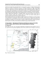
3. Case study II – Biomass growth (NPP) of Pinus pinaster and Eucalyptus
globulus stands, in the north of Portugal. Estimations by means of LANDSAT
ETM+ images
3.1 Study area
This research took place within an area in the northern part of Portugal where Pinus pinaster

Ait. and Eucalyptus globulus Labill constitute the two most important forest species in terms
of forested area (Figure 8).
The P. pinaster study area is a 60 km
2
rectangle (10 km × 6 km) with extensive stands of this
species located at the north of Vila Real (41°39′N, 7°35′W) and the E. globulus study area is a
24km
2
rectangle (4 km × 6 km) of extensive stands of this species located at west of Vila Real
(41°2′N, 7°43′W).
Both species are ecologically well adapted, despite E. globulus being an exotic tree, and the
case study areas are representative of these ecosystems in Portugal. The P. pinaster forest is
very heterogeneous in canopy density, has experienced only limited human intervention,
and covers a wide range of structures, varying widely in terms of number of trees per
hectare, average dimensions, and age groups. The E. globulus forest is much more
homogeneous and has been more extensively investigated to enable greater timber
production, which is very valuable for pulp production.


Fig. 8. Study area.
Assessment of Forest Aboveground Biomass Stocks and
Dynamics with Inventory Data, Remotely Sensed Imagery and Geostatistics

119
3.2 Methods and data
3.2.1 Methodology used in geometric and radiometric corrections
The available LANDSAT-7 ETM+ Image was acquired on the 15
th
of September 2001 at
10:02:13 (UTC). The image was geometrically and radiometrically corrected using MiraMon

("WorldWatcher"). This software allows displaying, consulting and editing raster and vector
maps and was developed by the Autonomous University of Barcelona (UAB) remote
sensing team. The software allows for the geometric correction of raster (e.g., IMG and JPG:
satellite images, aerial photos, scan maps) or vector maps (e.g., VEC, PNT, ARC and POL
and NOD), based on ground control points coordinates.
In the present research the ground control points were collected from Portuguese
topographic maps on a 1/25000-scale, using the original ETM+ Scene. Twenty-five control
points were collected (Toutin, 2004) to allow image correction and eleven control points
were used for its validation. A first-degree polynomial correction was chosen for the
geometric correction, using the nearest neighbour option for the resampling process.
Two Digital Elevation Models (DEMs) were constructed for each study area (Pinus
pinaster and Eucaliptus globulus – see Figure 8), based on 10 m contour lines. The first DEM
had a spatial resolution of 15 m and was used to correct the panchromatic band, mainly to
allow identification of the ground control points due to its better spatial resolution.
The second DEM had a spatial resolution of 20 m and was used for the correction of
the LANDSAT ETM+ bands 1, 2, 3, 4, 5, and 7. Those 20 m DEMs were merged with a
altitude model for Europe, with a pixel size of 1 Km. The radiometric correction was
based on the lowest radiometric value for each band which is well known as the kl, and
should be collected from the histogram analysis (Pons & Solé-Sugrañes, 1994 and Pons,
2002).
3.2.2 Methodology used to calculate vegetation indices
Within the study area, 31 sampling plots for the Eucalyptus globulus and 34 for the Pinus
pinaster were surveyed and the coordinates of the centre of each plot recorded by Global
Positioning System (GPS). The plots’ location could then be identified on the geo-corrected
images and reflectance data extracted for each ETM+ band. These data were then used to
calculate a series of vegetation indices (Table 5), which were further used to analyse
potential relationships with the forest variables.
In table 5, G represents the reflectance on the green wavelength; R is the reflectance in the
red wavelength; NIR is the reflectance in the near infrared wavelength; and MIR1 and MIR2
are the reflectance in the two middle infrared bands from LANDSAT ETM+ image.

3.2.3 Model adjustment and selection
The available data (31 sampling plots for the Eucalyptus globulus and 34 for the Pinus
pinaster) were divided in two groups, one for the adjustment of mathematical models and
the other for the validation. An overall analysis of the correlation matrix allowed to identify
the variables strongest related to NPP, which were then selected to establish regression
models to Estimate NPP. The best NPP prediction models were selected based in the
following statistics: the coefficient of determination (R
2
); the adjusted coefficient of
determination (R
2
adj.); the root mean square error (RMSE); and the percentage root mean
square error (RMSE%).

Progress in Biomass and Bioenergy Production

120
Designation
Mathematical
expression
Source

1

NDI(MIR1)
()
()
NIR MIR1
NIR MIR1
−

+


Lucas (1995)

2

NDI(MIR2)
()
()
NIR MIR2
NIR MIR2
−
+


Lucas (1995)

3

NDVI
()
()
NIR R
NIR R
−
+

Rouse et al. (1974); Bouman (1992); Malthus et al.
(1993); Xia (1994); Nemani et al. (1993); Baret et al.

(1995); Hamar et al. (1996); Fassnacht et al. (1997);
Purevdorj et al. (1998); Todd et al. (1998); and Singh
et al. (2003)

4

MVI1
MIR1
MIR2

Fassnacht et al. (1997)

5

MVI2
NIR
MIR2

Fassnacht et al.
(1997)

6

RVI1
NIR
R

Tucker (1979); Xia (1994); Baret
et al. (1995); Hamar
et al. (1996); Fassnacht et al. (1997); and Xu et al.

(2003).

7

TVI1
NIR
R


Tucker (1979)

8

TVI2
()
()
NIR R
NIR R
+
−


Tucker (1979)

9

TVI9
(G R)
0,5
(G R)

−
+
+


Tucker (1979)
Table 5. Vegetation indices used in the research
3.2.4 Comparison of the NPP images
NPP images obtained from different methodologies were compared by the Kappa index of
agreement. Kappa was adopted by the remote sensing community as a useful measure of
classification accuracy Rossiter (2004). The
Kappa coefficient (K) measures pairwise
agreement among a set of coders making category judgments, thus correcting values for
expected chance of agreement (Carletta, 1996).
The overall
kappa statistic, defining the overall proportion of area correctly classified, or in
agreement, is calculated by the mathematical expression defined by Eq. 9 (Stehman, 1997;
Rossiter, 2004):

kk
ii i i
i1 i1
k
ii
i1
pP.P
ˆ
k
1P.P
++

==
++
=
−
=
−


(9)
where:
Assessment of Forest Aboveground Biomass Stocks and
Dynamics with Inventory Data, Remotely Sensed Imagery and Geostatistics

121
k = number of land-cover categories
k
ii
i1
p
=

represents the overall proportion of area correctly classified
k
ii
i1
P.P
++
=

is the expected overall accuracy if there were chance agreement between reference

and mapped data
According to Green (1997) when there is complete agreement between two maps K=1, and a
kappa value of zero, the two maps are said to be unrelated.
Moss (2004) considers that when Kappa is less than 20 the strength of agreement between
both images is poor; between 0.21 and 0.40 fair; between 0.41 and 0.60 moderate; between
0.61 and 0.80 good; higher than 0.81 very good. However, according to Green (1997), kappa
lower than 0.40 indicates a low degree of agreement; between 0.40 and 0.75 a fair to good
degree of agreement; and higher than 0.75 a high degree of agreement.
3.3 Results and discussion
3.3.1 Identification of the best prediction variables
In order to identify whether if it was possible to directly or indirectly estimate NPP from the
remote sensing data, the Vegetation Index better correlated with NPP was identified from
the general correlation matrix and analysed. The most relevant results are summarised in
Table 6.


Pinus NPP Eucalyptus NPP
DN_B -0.179 -0.739
DN_G -0.268 -0.692
DN_R -0.194 -0.688
DN_NIR 0.344 -0.280
DN_MIR1 -0.078 -0.605
DN_MIR2 -0.174 -0.614
TVI2 -0.142 -0.535
TVI9 0.030 0.288
MVI1 0.486 0.427
MVI2 0.435 0.318
NDVI 0.280 0.519
NDI(MIR1) 0.181 0.386
NDI(MIR2) 0.232 0.466

Table 6. Correlation between NPP and the reflectance from each individual band and some
vegetation indices
As presented in Table 6,
Pinus NPP shows the higher correlation (positive) with the near
infrared wavelength band, while
Eucalyptus NPP is better correlated (negatively) whit the
middle infrared wavelength band.

Progress in Biomass and Bioenergy Production

122
The NDVI and TVI2 are the best correlated indices for the Eucalyptus and the MVI1 and
MVI2 for the
Pinus. These results reflect the initial observation when only reflectance from
each individual band was analysed.
The best correlated vegetation indices were selected as independent variables for adjusting
regression models to estimate NPP.
3.3.2 Models for the NPP Eucalyptus globulus estimation
The best mathematical models to estimate the NPP for the Eucalyptus stands and the basic
statistics (ME and MAE) calculated from the validation dataset are presented in Table 7.

Mathematical models
NPP adjusted
models statistics
Validation
dataset
statistics
R
2
R

2
ad
j
.
s
y
x
s
y
x
(%) ME MAE
NPP=27.644-0.243B-0.0007GR
2
-0.00014R
2
0.613 0.558 2.988 22.5 -1.631 2.758
NPP
arboreal
=89.260NDVI
2
-117.195NDVI
3

NPP=-13.114+12.271NPP
arboreal
-
1.818(NPP
arboreal
)
2

+0.091(NPP
arboreal
)
3

0.936
0.694
0.933
0.695
1.654
2.656
35.4
0.116
-1.198
1.238
3.098
NPP=3.593+167.750NDVI
2
-233.667NDVI
3
0.493 0.447 3.342 25.2 -0.340 2.959
NPP
litter
=56.584NDVI
2
-69.233NDVI
3

NPP=7.893(NPP
litter

)
0.412

0.812
0.678
0.805
0.666
2.088
2.484
53.0
18.7
-0.150
-0.589
1.309
2.834
NPP=17.672-0.611TVI2
2
+0.048TVI2
3
0.422 0.370 3.567 26.9 -0.347 2.903
G=13.431-155.484NDVI+648.846NDVI
2
-
635.713NDVI
3
NPP=-5.787+4.652G-0.339G
2
+0.008G
3

0.657

0.634
0.608

0.581
4.170

2.908
33.1

21.6
1.121

-0.779
2.687

3.347
G=38.150-0.300GR-0.174MIR1

NPP=-5.787+4.652G-0.339G
2
+0.008G
3

0.793
0.634
0.774
0.581
3.168

2.908
33.7
21.6
-1.754
-2.199
2.754
3.662
Table 7. Selected models to estimate Eucalyptus NPP, and validation dataset statistics
The observed standard error of the estimates are lower in the model using as independent
variable the blue, the green and the red reflectances, and in the model using the NDVI,
respectively. However, the model with NDVI as independent variable reveals a lower ME.
Additionally, this model has a superior applicability since the individual bands reflectance
have a great variation along the year, thus varying from image to image.
Based in the field measurements and in the estimated NPP, by the model using only the
NDVI directly as independent variable (R
2
=0.493), two images were created for the entire
study area (Figures 9a and 9b).
After the classification into four classes (1 – NPP < 5 ton ha
-1
year
-1
; 2- 5≤ NPP <10 ton ha
-
1
year
-1
; 3 - 10 ≤ NPP < 15 ton ha
-1
year

-1
; and 4 - NPP > 15 ton ha
-1
year
-1
) the cross tabulation
was carried out and the matrix error table analysed.
Kappa statistic showed a slight agreement around 37%. However, for a first approach these
results are a good indicator for further studies. From the analyses of the
Eucalyptus NPP
map, obtained from fieldwork, it can be observed that there are no areas with an NPP lower
than 5 ton ha
-1
year
-1
, and almost the whole Eucalyptus stand presents NPP figures between
10 and 15 ton ha
-1
year
-1
.
Assessment of Forest Aboveground Biomass Stocks and
Dynamics with Inventory Data, Remotely Sensed Imagery and Geostatistics

123


Fig. 9.
Eucalyptus NPP estimations from field measurements (a) and NDVI model (b).
A significant result to estimate

Eucalyptus NPP was obtained with the basal area (G) as
independent variable (R
2
=0.634). In this case, the basal area can be estimated with acceptable
confidence, using the NDVI or MIR1 as independent variables (R
2
=0.657 and 0.793,
respectively). In alternative,
Eucalyptus NPP can also be estimated indirectly, with
acceptable accuracies, by the litter present in the
Eucalyptus stands (R
2
=0.678). A strong
relationship was found between NPP from litter and NDVI (R
2
=0.812). The same
methodology can be used by estimating, in a previous stage, the NPP arboreal with the
NDVI as independent variable (R
2
=0.936) and subsequently, indirectly estimate the
Eucalyptus NPP (R
2
=0.694).
3.3.3 Models for the NPP Pinus pinaster estimation
The best mathematical models to estimate the NPP for the Pinus stands and the basic
statistics (ME and MAE) calculated from the validation dataset are presented in Table 8. The
observed standard error of the estimates, as well the ME achieved from the validation
dataset shows that the best model is obtained in the model using as independent variable
the MVI1 for estimate the NPP of shrubs. The NPP of pine is subsequently estimated
indirectly using this variable.

As in the
Eucalyptus predictions the same methodology was implemented to compare the
final maps achieved for the Pinus stands. The
Pine NPP model using only the MVI1 as
independent variable was used (R
2
=0.417). The two created maps for the entire study area
(Figures 10a and 10b), were classified into four classes (1 – NPP < 5 ton ha
-1
year
-1
; 2- 5≤ NPP
<10 ton ha
-1
year
-1
; 3 - 10 ≤ NPP < 15 ton ha
-1
year
-1
; and 4 - NPP > 15 ton ha
-1
year
-1
), a cross
tabulation was carried out and the matrix error table analysed. Kappa statistic showed an
(a)
(b)

Progress in Biomass and Bioenergy Production

124
agreement around 48%, slightly better than in Eucalyptus estimations. However, it was
observed that the achieved model was not able to identify and locate the extreme values of
NPP (e.g. neither the most productive areas nor the least productive ones).

Mathematical models
NPP adjusted
models statistics
Validation
dataset
statistics
R
2
R
2
ad
j
.
s
y
x
s
y
x
(%) ME MAE
NPP=51.288-32.080MVI1+6.787MVI1
2
0.417 0.369 4.617 31.7 -0.902 1.974
NPP

shrubs
=-0.516MVI1
2
+0.414MVI1
3

NPP=10.629+1.071NPP
shrubs

0.816
0.649
0.809
0.635
2.614
3.508
71.3
27.5
-0.279
-0.317
2.146
1.677
NPP
shrubs
=1.146+0.142MVI2
2
NPP=10.629+1.071NPP
shrubs

0.486
0.649

0.466
0.635
3.196
3.508
83.8
27.6
-0.490
-0.842
2.268
2.276
Table 8. Selected models to estimate Pinus NPP and validation dataset statistics




Fig. 10. Pinus NPP estimations from field measurements (a), and the MVI1 model (b).
For the
Pinus stands, it was possible to estimate the total NPP (R
2
=0.816) knowing only the
NPP from shrubs. In this case, the NPP from shrubs was predicted using the MVI as
auxiliary variable (R
2
=0.645).
(a)
(b)
Assessment of Forest Aboveground Biomass Stocks and
Dynamics with Inventory Data, Remotely Sensed Imagery and Geostatistics

125

4. Conclusions
In this research, AGB and NPP estimates were carried out by means of forest inventory data
remote sensing imagery and geostatistical modeling. The general conclusions are:
In the case study I, tree Aboveground biomass (AGB) mapping approaches were
compared: Inventory Polygons; Direct Radiometric Relationships (DRR) and Regression-
kriging (RK). Pure pine stands were mapped and AGB estimates were achieved using
data collected in the National Forest inventory dataset. The Inventory polygons method
was used since the field plots of forest inventory dataset fall within all the polygons of the
forest cover map. At the same time, this approach was used to compare and validate DRR
and RK methods.
The results showed that DRR and RK, using Vegetation Indices transformed from MODIS
remotely sensed data, can be used for biomass mapping purposes. However, it should be
pointed out that, in the present research, the coarse resolution of MODIS (250m) data
associated with small polygons of the pine landcover class did not allow to extract the pure
spectral response of this vegetation type. Hence, the correlation between AGB and NDVI as
independent variable is not as high as desired.
This limitation can be overcome by using images with higher spatial resolution. Moreover,
these methodologies can be applied with greater accuracy in areas where land cover
polygons are large enough to minimize, as much as possible, the effect of edging.
The analysis of statistical parameters of validation dataset such as the mean error (ME), the
mean absolute error (MAE), standard deviation (SD) and the root mean squared error
(RMSE) show that RK, making use of geostatistical modeling techniques, combined with
remote sensing data as auxiliary variable improves the predictions when compared to DRR.
Furthermore, RK has the advantage of generating estimates for the spatial distribution of
AGB and its uncertainty for the study area. The uncertainty maps allow the evaluation of
the reliability of estimates by identifying the sites with major uncertainties which can be
useful to select different estimation methods for those areas.
In the case study II, some simplified methodologies were proposed to estimate NPP. For the
Eucalyptus ecosystem using the basal area or the NPP from litter, and for the Pinus
ecosystem using the NPP from shrubs.

Despite the direct NPP estimation from remote sensing data did not provide very promising
results, it was possible to establish indirect relationships between some vegetations indices
calculated from Landsat ETM+ imagery data and the litter NPP, shrubs NPP and from basal
area of the studied forest stands.
Those simplifications can be extremely important when time and economic resources are
limited. The importance of those methodologies could become more relevant as NPP is a
variable very difficult to obtain, consuming time and demanding hard fieldwork.
The loss in accuracy is certainly compensated by decrease of fieldwork. The balance between
both should only be taken in each particular case, considering the general context of each
situation (e.g., time and funds available, human resources available, objectives of the research).
5. Acknowledgements
Authors would like to express their acknowledgement to the Portuguese Science and
Technology Foundation (FCT), programmes SFRH/PROTEC/49626/2009 and FCT FCOMP-
01-0124-FEDER-007010 (PTDC/AGR-CFL/68186/2006).

Progress in Biomass and Bioenergy Production

126
6. References
AFN (2006). Dados do Inventário Florestal Nacional (05/06) Information retrieval tool.
Autoridade Florestal Nacional. Ministério da Agricultura do Desenvolvimento
Rural e das Pescas, Lisboa.
Ahmed, S., & de Marsily, G (1987). Comparison of geostatistical methods for estimating
transmissivity using data on transmissivity and specific capacity.
Water Resources
Research
23(9): 1717-1737.
Atkinson, P. M.; Foody, G. M.; Curran, P. J., & Boyd D. S. (2000). Assessing the ground data
requirements for regional scale remote sensing of tropical forest biophysical
properties.

International Journal of Remote Sensing 21(13-14): 2571-2587.
Baret, F., Clevers, J.G. and Steven, M.D. (1995). The robustness of canopy gap fraction
estimates from red and near-infrared reflectances: A comparison of approaches.
Remote Sensing of Environment 54: 141-151.
Bouman, B.M. (1992). Accuracy of estimating the leaf area index from vegetation indices
derived from crop reflectance characteristics: a simulation study.
International
Journal of Remote Sensing
13(16): 3069-3084.
Burcsu, T. K., Robeson, S. M., & Meretsky, V.J. (2001). Identifying the Distance of Vegetative
Edge Effects Using Landsat TM Data and Geostatistical Methods.
Geocarto
International
16( 4): 61-70.
Cao, M. and Woodward, F.I. (1998). Net primary and ecosystem production and carbon
stocks of terrestrial ecosystems and their responses to climate change.
Global Change
Biology
4: 185-198.
Carletta, J. (1996). Assessing agreement on classification tasks: the kappa statistic.
Computational linguistics 22(2): 1-6.
Chirici, Gherardo; Barbati, Anna, & Maselli, Fabio (2007). Modelling of Italian forest net
primary productivity by the integration of remotely sensed and GIS data.
Forest
Ecology and Management
246: 285-295.
Cressie, N. A. C. (1993).
Statistics for Spatial Data. New York, USA: John Wiley & Sons. pp.
416.
Curran, P.J. (1988). The semivariogram in remote sensing: An introduction.

Remote Sensing of
Environment
24: 493-507.
Deutsch, C. V., & Journel A. G. (1998).
Geostatistical Software Library and User’s Guide. (2nd
ed.). New York, USA: Oxford University Press, pp. 369.
Eastman, J. R. (2006).
Idrisi Andes. Guide to GIS and Image Processing. USA: Clark Labs. Clark
University, pp. 328.
Fassnacht, K.S., Gower, S.T., MacKenzie, M.D., Nordheim, E.V. and Lillesand, T.M. (1997).
Estimating the leaf area index of north central Wisconsin forests using the Landsat
Thematic Mapper.
Remote Sensing of Environment 61: 229-245.
Field, C.B., Randerson, J.T. and Malmstrom, C.M. (1995). Global net primary production:
combining ecology and remote sensing.
Remote Sensing of Environment 51: 74-88.
García-Martín, A., Pérez-Cabello, F., de la Riva, J. R., & Montorio, R. (2008). Estimation of
crown biomass of Pinus spp. from Landsat TM and its effect on burn severity in a
Spanish fire scar.
IEEE Journal of Selected Topics in Applied Earth Observations and
Remote Sensing 1
(4): 254-265.
Goovaerts, P. (1997).
Geostatistics for Natural Resources Evaluation. New York, USA: Oxford
University Press, Inc., pp. 496.
Assessment of Forest Aboveground Biomass Stocks and
Dynamics with Inventory Data, Remotely Sensed Imagery and Geostatistics

127
Goovaerts, P. (1999). Using elevation to aid the geostatistical mapping of rainfall erosivity.

Catena 34(3-4): 227-242.
Green, A.M. (1997). Kappa statistics for multiple raters using categorical classifications,
Proceedings of the twenty-second annual SAS @Users Group International Conference,
Cary, NC: SAS Institute, Inc: 1110-1115.
Hamar, D., Ferencz, C., Lichtenberger, J., Tarcsa, G. and Ferencz-Árkos, I. (1996). Yield
estimation for corn and wheat in the hungarian great plain using landsat MSS data.
International Journal of Remote Sensing 17(9): 1689-1699.
Häme, T., Salli, A., Andersson, K., & Lohi, A. (1997). A new methodology for estimation of
biomass of conifer-dominated boreal forest using NOAA AVHRR data.
International Journal of Remote Sensing 18: 3211-3243.
Hengl T., Heuvelink G. M. B., & Stein A. (2004). A generic framework for spatial prediction
of soil variables based on regression-kriging.
Geoderma 122(1-2): 75-93.
Hengl T., Heuvelink, G. B. M. & Rossiter, D. G. (2007). About regression-kriging: from
equations to case studies.
Computers and Geosciences 33(10): 1301-1315.
Hengl, T. (2009).
A Practical Guide to Geostatistical Mapping. Amsterdam, ISBN 978-90-
9024981-0.
Hese, S., Lucht, W., Schmullius, C., Barnsley, M., Dubayah, R., Knorr, D., Neumann, K.,
Riedel, T., & Schröter, K. (2005). Global biomass mapping for an improved
understanding of the CO2 balance-the Earth observation mission Carbon-3D.
Remote Sensing of Environment 94(1): 94-104.
Hu, Huifeng, & Wang, G. G. (2008). Changes in forest biomass carbon storage in the South
Carolina Piedmont between 1936 and 2005.
Forest Ecology and Management 255(5-6):
1400-1408.
Hyde, P., Nelson, R., Kimes, D., & Levine, E. (2007). Exploring LiDAR–RaDAR synergy-
predicting aboveground biomass in a southwestern ponderosa pine forest using
LiDAR, SAR and InSAR.

Remote Sensing of Environment 106(1): 28-38.
IGP (2010).
CLC2006 – Cartografia CORINE Land Cover 2006 para Portugal Continental; 2009.
< (verified 01.01.2010).
Isaaks, E. H., & Srivastava, R. M. (1989).
An Introduction to Applied Geostatistics. New York,
USA: Oxford University Press, pp. 542.
Jarlan, L., Mangiarotti, S., Mougin E., Mazzega, P., Hiernaux, P., & Le Dantec, V. (2008).
Assimilation of SPOT/VEGETATION NDVI data into a sahelian vegetation
dynamics model.
Remote Sensing of Environment 112(4): 1381-1394.
Knotters, M., Brus, D. J., & Voshaar, J. H. O. (1995). A comparison of kriging, co-kriging and
kriging combined with regression for spatial interpolation of horizon depth with
censored observations.
Geoderma 67(3-4): 227–246.
Labrecque, S., Fournier, R. A., Luther, J. E., & Piercey, D. (2006). A comparison of four
methods to map biomass from Landsat-TM and inventory data in western
Newfoundland.
Forest Ecology and Management 226, 129-144.
Liao, J., Dong, L., & Shen, G. (2009). Neural network algorithm and backscattering model for
biomass estimation of wetland vegetation in Poyang Lake area using Envisat ASAR
data.
Geoscience and Remote Sensing Symposium, IEEE International, IGARSS 2009.
Lloyd, C. D. (2007).
Local Models for Spatial Analysis. Boca Raton: CRC Press, Taylor & Francis
Group.

Progress in Biomass and Bioenergy Production

128

Lu, D. (2006). The potential and challenge of remote sensing-based biomass estimation.
International Journal of Remote Sensing 27: 1297-1328.
Lucas, N.S. (1995).
Coupling remotely sensed data to a forest ecosystem simulation model. Thesis
for the Degree of Doctor of Philosophy, University of Wales, Swansea, England, pp.
375.
Madugundu, R.; Nizalapur, V. & Jha, C. S. (2008). Estimation of LAI and above-ground
biomass in deciduous forests: Western Ghats of Karnataka, India.
International
Journal of Applied Earth Observation and Geoinformation
10(2): 211-219.
Malthus, T.J., Andrieu, B., Danson, F.M., Jaggard, K.W. and Steven, M.D. (1993). Candidate
high spectral resolution infrared indices for crop cover.
Remote Sensing of
Environment
46: 204-212.
Matheron G. (1963). Principles of geostatistics.
Economic Geology 58: 1246–1266.
Matheron G. (1971).
The theory of regionalised variables and its applications. Les Cahiers du Centre
de Morphologie Mathematique de Fontainblue
. Paris: Ecole Nationale Superiore de
Paris, pp. 212.
Melillo, J.M, McGuire, A.D., Kicklighter, D.W., Moore III, B., Vorosmarty, C.J. and Schloss,
A.L. (1993). Global climate change and terrestrial net primary production.
Nature
363: 234-240.
Meng, Q., Cieszewski, C. J., Madden, M., & Borders, B. E. (2007). K Nearest Neighbor
method for forest inventory using remote sensing data.
GIScience & Remote Sensing

44(2): 149-165.
Meng, Q.; Cieszewski, C. J. & Madden, M. (2009). Large area forest inventory using Landsat
ETM+: A geostatistical approach.
ISPRS Journal of Photogrammetry and Remote
Sensing
64: 27-36.
Moss, S. (2004). Kappa statistics. The Institute of Cancer Research,

Muukkonen, P., & Heiskanen, J. (2007). Biomass estimation over a large area based on
standwise forest inventory data and ASTER and MODIS satellite data: A possibility
to verify carbon inventories.
Remote Sensing of Environment 107: 617–624.
Nemani, R., Pierce, L., Running, S. and Band, L. (1993). Forest ecosystem processes at the
watershed scale: sensitivity to remotely-sensed leaf area index estimates.
International Journal of Remote Sensing 14(13): 2519-2534.
Odeh, I. O. A., McBratney, A. B., & Chittleborough, D. J. (1994). Spatial prediction of soil
properties from landform attributes derived from a digital elevation model.
Geoderma, 63: 197-214.
Odeh, I.O. A., McBratney, A. B., & Chittleborough, D. J. (1995). Further results on prediction
of soil properties from terrain attributes: heterotopic cokriging and regression-
kriging.
Geoderma 67(3-4): 215–226.
Palmer, D. J.; Höck, B. K.; Kimberley, M. O.; Watt, M. S.; Lowe, D. J. & Payn, T. W. (2009).
Comparison of spatial prediction techniques for developing Pinus radiate
productivity surfaces across New Zealand.
Forest Ecology and Management 258: 2046-
2055.
Pebesma, E. (2001).
Gstat user’s manual. University of Utrecht, pp. 108.
Pebesma, E. (2004). Multivariable geostatistics in S: the gstat package. Computers &

Geosciences 30(7): 683-691.
Assessment of Forest Aboveground Biomass Stocks and
Dynamics with Inventory Data, Remotely Sensed Imagery and Geostatistics

129
Pons, X and Solé-Sugrañes, L. (1994). A simple radiometric correction model to improve
automatic mapping of vegetation from multispectral satellite data.
Remote Sensing of
Environment
48: 191-204.
Pons, X. (2002).
MiraMon. Geographic information system and remote sensing software Centre de
Recerca Ecològica i Aplicacions Forestals, CREAF. Bellaterra. ISBN: 84-931323-5-7.
Purevdorj, T., Tateishi, R., Ishiyamas, T., and Honda, Y. (1998). Relationships between
percent cover and vegetation indices.
International Journal of Remote Sensing 19(18):
3519-3535.
Rahman, M. M.; Csaplovics, E., & Koch, B. (2005). An efficient regression strategy for
extracting forest biomass information from satellite sensor data.
International Journal
of Remote Sensing
26(7): 1511-1519.
Rossiter, D.G. (2004).
Statistical method for accuracy assessment of classified thematic map.
International Institute for Geo-information Science and Earth, Department of Earth
Systems Analysis, Enschede, NL, pp. 46.
Rouse, J.W., Haas, R.H., Schell, J.A., Deering, D.W. and Harlan, J.C. (1974).
Monitoring the
vernal advancement retrogradiation of natural vegetation
. Final Report Type III,

NASA/GSFC, Greenbelt, MD., USA, pp. 371.
Sales, M. H., Souza Jr., C. M., Kyriakidis, P. C.; Roberts, D. A., & Vidal, E. (2007). Improving
spatial distribution estimation of forest biomass with geostatistics: A case study for
Rondônia, Brazil.
Ecological Modelling 205: 221-230.
Sen, Zekai (2009).
Spatial Modeling Principles in Earth Sciences. London, New York: Springer
Dordrecht Heidelberg, pp. 351.
Singh, R.P., Roy, S., and Koogan, F. (2003). Vegetation and temperature condition indices
from NOAA AVHRR data for drought monitoring over India.
International Journal
of Remote Sensing
24 (22): 4393-4402.
Stehman, S.V. (1997). Selecting and interpreting measures of thematic classification
accuracy.
Remote Sensing of Environment 62: 77-89.
Todd, S.W., Hoffer, R.M., and Milchunas, D.G. (1998). Biomass estimation on grazed and
ungrazed rangelands using spectral indices.
International Journal of Remote Sensing
19 (3): 427-438.
Tomppo, E. (1991). Satellite imagery-based national inventory of Finland.
International
Archives of Photogrammetry and Remote Sensing 28
(7-1): 419-424.
Tomppo, E., Nilsson, M., Rosengren, M., Aalto, P., Kennedy, P. (2002). Simultaneous use of
Landsat-TM and IRS-1c WiFS data in estimating large area tree stem volume and
aboveground biomass.
Remote Sensing of Environment 82: 156−171.
Toutin, T. (2004). Review article: Geometric processing of remote sensing images: models,
algorithms and methods.

International Journal of Remote Sensing 25(10): 1893-1924.
Tucker, C.J. (1979). Red and photographic infrared linear combinations for monitoring
vegetation.
Remote Sensing of Environment 8: 127-150.
Waring, R.H., Landsberg, J.J. and Williams, M. (1998). Net primary production of forests: a
constant fraction of gross primary production?
Tree Physiology 18: 129-134.
Webster, R. & Oliver, M. A. (1992). Sample adequately to estimate variograms of soil
properties.
Journal of Soil Science 43: 177-192.
Webster, R. & Oliver, M. A. (2007).
Geostatistics for Environmental Scientists. (2nd ed.),
England: John Wiley & Sons Ltd, pp.332.

Progress in Biomass and Bioenergy Production

130
Woodcock, C. E, Strahler, A. H., & Jupp, D. L. B. (1988). The use of variograms in remote
sensing: II. Real digital images.
Remote Sensing of Environment 25: 349-379.
Xia, L., 1994. A two-axis adjusted vegetation index (TWVI).
International Journal of Remote
Sensing
15(7): 1447-1458.
Xu, B., Gong, P., and Pu, R. (2003). Crown closure estimation of oak savannah in a dry
season with Landsat TM imagery: comparison of various indices through
correlation analysis.
International Journal of Remote Sensing 24 (9): 1811-1822.
Zheng, D., Heath, L. S., & Ducey, M. J. (2007). Forest biomass estimated from MODIS and
FIA data in the. Lake States: MN, WI and MI, USA.

Forestry 80(3): 265-278.
Part 3
Metal Biosorption and Reduction

7
Hexavalent Chromium
Removal by a Paecilomyces sp Fungal
Juan F. Cárdenas-González and Ismael Acosta-Rodríguez
Universidad Autónoma de San Luis Potosí, Facultad de Ciencias Químicas,
Centro de Investigación y de Estudios de Posgrado, Laboratorio de Micología Experimental
S.L.P. México
1. Introduction
The strong impact of hexavalent chromium on the environment and on the human health
demand suitable technologies to neutralize the hazard of chromium. The traditional
technologies used for the remediation of environment contaminated with Cr (VI) are based
on physical and chemical approaches, which require large amounts of chemical substances
and energy. Such methodologies have proved complete expensive on a large-scale
application at contaminated sites, and also they have generated hazardous by-products
(Cervantes et. al., 2001). Bioremediation, a strategy that uses living microorganisms, is
essentially proposed to clean up the environment from organic pollutants. However, since
there is an evidence that several microorganisms possess the capability to reduce Cr (VI) to
relatively toxic Cr (III), bioremediation gives immense opportunities for the development of
technologies for the detoxification of soil contaminated with Cr (VI) as an alternative to
existing physical-chemical remediation technologies (Cervantes et al., 2001).
Chromium is an essential micro-nutrient in the diet of animals and humans, as it is
indispensable for the normal sugar, lipid and protein metabolism of mammals. Its
deficiency in the diet causes alteration in lipid and glucose metabolism in animals and
humans. Chromium is included in the complex named glucose tolerance factor (GFC)
(Armienta-Hernández and Rodríguez-Castillo, 1995). On the other hand, no positive effects
of chromium are known in plants and microorganisms. However, elevated levels of

chromium are always toxic, although the toxicity level is related to the chromium oxidation
state. Cr (VI) not only is highly toxic to all forms of living organisms. It is mutagenic for
bacteria, mutagenic and carcinogenic for humans and animals, but also, it is involved in
causing birth defects and the decrease of reproductive health (Marsh and McInerney, 2001).
This metal may cause death in animals and humans, if ingested in large doses. The LD
50
for
oral toxicity in rats is from 50 to 100 mg/kg for Cr (VI) and 1900-3000 mg/kg for Cr (III). Cr
(VI) toxicity is related to its easy diffusion across the cell membrane in prokaryotic and
eukaryotic organisms and subsequent Cr (VI) reduction in cells, which gives free radicals
that, may directly cause DNA alterations as well as toxic effects. Cr (III) has been estimated
to be from 10 to 100 times less toxic than Cr (VI), because cellular membranes appear to be
quite impermeable to most Cr (III) complexes. Nevertheless, intracellular Cr (III), which is
the terminal product of the Cr (VI)-reduction, forms amino acid nucleotide complexes in
vivo, whose mutagenic potentiality is not fully known (Gutiérrez Corona, et al., 2010).