Progress in Biomass and Bioenergy Production Part 7 pptx
Bạn đang xem bản rút gọn của tài liệu. Xem và tải ngay bản đầy đủ của tài liệu tại đây (686.71 KB, 30 trang )
Biosorption of Metals: State of the Art, General Features, and
Potential Applications for Environmental and Technological Processes
169
0 5000 10000 15000 20000 25000
0,0
0,2
0,4
0,6
0,8
1,0
C/C
0
t
(
min
)
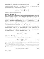
Fig. 8. Modeling of breakthrough curve in the column biosorption of La(III) for
Sargassum sp. biomass by the Thomas model. Symbols: (■) data of metal concentration on
eluate and (––) curve fit for Thomas model. Source: Oliveira, 2011.
6.2 Dependence of the operational parameters
There is broad literature that describes the effects of operational parameters to augment and
to improve the biosorption in fixed-bed columns (Chu, 2004; Hashim & Chu, 2004;
Kratochvil & Volesky, 2000; Naddafi et al., 2007; Oliveira, 2007; Oliveira, 2001; Valdman et
al., 2001; Vieira et al., 2008; Vijayaraghavan et al., 2005; Vijayaraghavan et al., 2008;
Vijayaraghavan & Prabu, 2006; Volesky et al., 2003). These parameters modified mainly
related are: flow rate, feeding concentration, height of packed-bed column, porosity, mass of
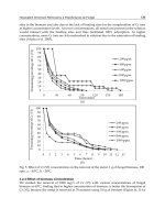
biomass, etc. Vijayaraghavan & Prabu (2006) evaluate some variables as the bed height (15
to 25 cm), flow rate (5 to 20 mL/min), and copper concentration (50 to 100 mg/L) in
Sargassum wightii biomass from breakthrough curves: each variable evaluated was changed
and the others were fixed. Continuous experiments revealed that the increasing of the bed
height and inlet solute concentration resulted in better column performance, while the
lowest flow rate favored the biosorption (Vijayaraghavan & Prabu, 2006)
Naddafi et al. (2007) studied the biosorption of binary solution of lead and cadmium in
Sargassum glaucescens biomass from the breakthrough curves modeled according with the
Thomas model (eq. (7)). Under selected flow rate condition (1.5 L/h) the experiments
reached a selective biosorption. The elution of the metals in distinct breakthrough times
with biosorption uptake in these times at 0.97 and 0.15 mmol/g for lead and cadmium,
respectively.
6.3 Desorption: chromatographic elution and biomass reuse
Column desorption is used for the metal recovery, but this procedure under selected
conditions may be operated to carry out chromatographic elution by the displacement of the
adsorbed components in enriched fractions containing each metal (Diniz & Volesky, 2006).
This is resulted of the simple drag of the previous separation on frontal analysis.
Nevertheless the eluent may present differential affinity by the adsorbed solutes, so there is
Progress in Biomass and Bioenergy Production
170
the possibility to use the procedure to promote a more effective separation of the
components. The chromatographic elution is dependent of the parameters referred to frontal
analysis and of the composition and concentration of the displacement solution. Desorption
profiles are given as bands or peaks whose modeling are associated directly to mathematic
approximations by Gaussian functions that may be modified or not exponentially
(Guiochon et al., 2006).
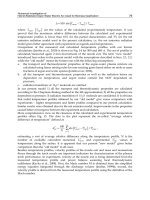
A typical column desorption with hydrochloric acid from Sargassum sp. previously
submitted to biosorption of lanthanum is showed on Fig. 9, which is represented by
lanthanum concentration in eluate as function of the volume.
0 200 400 600 800 1000
0
1
2
3
4
5
[La
3+
] / g L
-1
V / mL
Fig. 9. Column desorption of La(III) from Sargassum sp. biomass with HCl 0.10 mol/L.
Symbols: (–■–) metal concentration on eluate. Source: Oliveira, 2011.
On Fig. 9 can be seen that after the start of the acid percolation occurs a quick increase of
concentration until the maximum to 5.08 g/L for lanthanum. Parameters as the recovery
percentage (p) and concentration factor (f) are obtained from biosorption and desorption
curves. The recovery percentage is resulted of the ratio between the values of metal recovery
on desorption and maximum metal uptake on biosorption, while the concentration factor
refers to the ratio between the saturation volume on biosorption and the effective recovery
volume on desorption. Both measure the efficiency of the desorbing agents in the metal
recovery. For instance, these parameters obtained from Fig. 9 were 93.3% and 60.4 times of
recovery percentage and concentration factor, respectively; which are expressive and
satisfactory for the column biosorption purposes (Oliveira, 2011).
For biosorption and desorption processes, other important aspect is the biosorbent reuse for
recycles biosorption-desorption according the cost benefit between the biosorption capacity
loss during desorption steps and the metal recuperation operational yield (Diniz & Volesky,
2006; Gadd, 2009; Godlewska-Zylkiewicz, 2006; Gupta & Rastogi, 2008; Volesky et al., 2003).
Oliveira (2007) performed the neodymium column biosorption by Sargassum sp. and the
subsequent desorption in three recycles. In these experiments was observed that occurs a
Biosorption of Metals: State of the Art, General Features, and
Potential Applications for Environmental and Technological Processes
171
decrease in mass metal accumulation through the cycles. Accumulation decrease from first
to third cycle in 22%, which is due to the partial destruction of binding sites on desorption
procedures, and the binding sites blocking by neodymium ions strongly adsorbed. The
result showed that the biomass may be used for recycle finalities.
The loss in performance of the adsorption during the recycles can has numerous origins.
Generally they are associated to the modifications on chemistry and structure of the
biosorbent (Gupta & Rastogi, 2008), and the changes of access conditions of the desorbent to
the metal and mass transfer. Low-grade contaminants in the solutions used in these
procedures may accumulate and to block the binding sites or to affect the stability of these
molecules (Volesky et al., 2003).
7. References
Ahluwalia, S. S. & Goyal, D. (2007). Microbial and plant derived biomass for removal of
heavy metals from wastewater. Bioresource Technology, Vol.98, No.12, (September
2007), pp. 2243-2257, ISSN 0980-8524.
Aksu, Z. (2001). Equilibrium and kinetic modeling of cadmium (II) biosorption by C. vulgaris
in a batch system: effect of temperature. Separation and Purification Technology,
Vol.21, No.3, (January 2001), pp. 285-294, ISSN 1383-5866.
Aksu, Z. & Açikel, Ü. (2000). Modeling of a single-staged bioseparation process for
simultaneous removal for iron(III) and chromium(VI) by using Chlorella vulgaris.
Biochemical Engineering Journal, Vol.4, No.3, (February 2000), pp. 229-238, ISSN 1369-
703X.
Andrès, Y.; Thouand, G.; Boualam, M. & Mergeay, M. (2000). Factors influencing the
biosorption of gadolinium by microorganisms and its mobilization from sand.
Applied Microbiology and Biotechnology, Vol.54, No.2, (August 2000), pp. 262-267,
ISSN 0175-7598.
Arica, M.; Bayramoglu, G.; Yilmaz, M.; Bektas, M. & Genç, O. (2004). Biosorption of Hg
2+
,
Cd
2+
, and Zn
2+
by Ca-alginate and immobilized wood-rotting fungus Funalia trogii.
Journal of Hazardous Materials, Vol.109, No.1-3, (June 2004), pp. 191-199, ISSN 0304-
3894.
Atkinson, B. W.; Bux, F. & Kasan, H. C. (1998). Considerations for application of biosorption
technology to remediate metal-contaminated industrial effluents. Water S.A.,
Vol.24, No.2, (April 1998), pp. 129-135, ISSN 0378-4738.
Benaissa, H & Benguella, B. (2004). Effect of anions and cations on cadmium sorption
kinetics from aqueous solutions by chitin: experimental studies and modeling.
Environmental Pollution, Vol.130, No.2 , (July 2004), pp. 157-163, ISSN 0269-7491.
Bruins, M. R.; Kapil, S. & Oehme, F. W. (2000). Microbial resistance to metals in the
environment. Ecotoxicology and Environmental Safety, Vol.45, No.3, (March 2000), pp.
198-207, ISSN 0147-6513.
Chu, K. H. (2004). Improved fixed bed models for metal biosorption. Chemical Engineering
Journal, Vol.97, No.2-3, (February 2003), pp. 233-239, ISSN 1385-8947.
Crini, G. (2005). Recent developments in polysaccharide-based materials used as adsorbents
in wastewater treatment. Progress in Polymer Science, Vol.30, No.1, (January 2005),
pp. 38-70, ISSN 0079-6700.
Progress in Biomass and Bioenergy Production
172
Dambies, L.; Guimon, C.; Yiacoumi, S. & Guibal, E. (2000). Characterization of metal ion
interactions with chitosan by X-ray photoelectron spectroscopy. Colloids and
Surfaces A: Physicochemical and Engineering Aspects, Vol.177, No.2-3, (February 2000),
pp. 203-214, ISSN 0927-7757.
Deng, S. & Bai, R. (2004). Removal of trivalent and hexavalent chromium with aminated
polyacrylonitrile fibers: performance and mechanisms. Water Research, Vol.38, No.9,
(May 2004), pp. 2424-2432, ISSN 0043-1354.
Diniz, V. & Volesky, B. (2005). Biosorption of La, Eu and Yb using Sargassum biomass. Water
Research, Vol.39, No.1, (January 2005), pp. 239-247, ISSN 0043-1354.
Diniz, V. & Volesky, B. (2006). Desorption of lanthanum, europium and ytterbium from
Sargassum. Separation and Purification Technology, Vol.50, No.1, (June 2006), pp. 71-
76, ISSN 1383-5866.
Dos Santos, V. C. G., De Souza, J. V. T .M., Tarley, C. R. T., Caetano, J. & Dragunsky, D. C.
(2011). Copper ions adsorption from aqueous medium using the biosorbent
sugarcane bagasse in natura and chemically modified. Water, Air & Soil Pollution,
Vol.216, No.1-4, (March 2011), pp. 351-359, ISSN 0049-6979.
Eccles, H. (1999). Treatment of metal-contamined wastes: why select a biological process?
Trends in Biotechnology, Vol.17, No. 12, (December 1999),pp. 462-465, ISSN 0167-
7799.
Freitas, O. M. M.; Martins, R. J. E.; Delerue-Matos, C. M. & Boaventura, R. A. R. (2008).
Removal of Cd(II), Zn(II) and Pb(II) from aqueous solutions by brown marine
macro algae: Kinetic modeling. Journal of Hazardous Materials, Vol.153, No.1-2, (May
2008), pp. 493–501, ISSN 0304-3894.
Gadd, G. M. (2009). Biosorption: critical review of scientific rationale, environmental
importance and significance for pollution treatment. Journal of Chemical Technology
& Biotechnology, Vol.84, No.1, (January 2009), pp. 13-28, ISSN 1097-4660.
Ghimire, K. N.; Inoue, K.; Ohto, K. & Hayashida, T. (2008). Adsorption study of metal ions
onto crosslinked seaweed Laminaria japonica. Bioresource Technology, Vol.99, No.1,
(January 2008), pp. 32-37, ISSN 0980-8524.
Godlewska-Zylkiewicz, B. (2006). Microorganisms in inorganic chemical analysis. Analytical
and Bioanalytical Chemistry, Vol.384, No.1, (January 2006), pp. 114-123, ISSN 1618-
2642.
Guiochon, G.; Felinger, A.; Shirazi, D. G. & Katti, A. M. (2006). Fundamentals of preparative
and nonlinear chromatography (2nd ed.), Academic Press, ISBN 978-0-12-370537-2,
Boston, USA.
Gupta, V. K. & Rastogi, A. (2008). Equilibrium and kinetic modeling of cadmium(II)
biosorption by nonliving algal biomass Oedogonium sp. from aqueous phase. Journal
of Hazardous Materials, Vol.153, No.1-2, (May 2008),pp. 759-766, ISSN 0304-3894.
Hashim, M. A. & Chu, K. H. (2004). Biosorption of cadmium by brown, green, and red
seaweeds. Chemical Engineering Journal, Vol. 97, No.2-3, (February 2004), pp. 249-
255, ISSN 1385-8947.
Karnitz Jr., O. (2007). Modificação química do bagaço de cana e celulose usando anidrido do EDTA.
Uso destes materiais na adsorção de metais pesados em solução aquosa, MSc Thesis,
Biosorption of Metals: State of the Art, General Features, and
Potential Applications for Environmental and Technological Processes
173
Instituto de Ciências Exatas e Biológicas, Universidade Federal de Ouro Preto,
Ouro Preto, Brazil.
Kentish, S. E. & Stevens, G. W. (2001). Innovations in separations technology for the
recycling and re-use of liquid waste streams. Chemical Engineering Journal, Vol.84,
No.2, (October 2001), pp. 149-159, ISSN 1385-8947.
Kratochvil, D. & Volesky, B. (2000). Multicomponent biosorption in fixed beds. Water
Research, Vol.34, No.12, (August 2000), pp. 3186-3196, ISSN 0043-1354.
Lin, Z.; Zhou, C.; Wu, J.; Zhou, J. & Wang, L. (2005). A further insight into the mechanism of
Ag
+
biosorption by Lactobacillus sp. strain A09. Spectrochimica Acta Part A: Molecular
and Biomolecular Spectroscopy, Vol. 61, No.6, (April 2005), pp. 1195-1200, ISSN 1386-
1425.
Liu, Y. & Liu, Y J. (2008). Biosorption isotherms, kinetics and thermodynamics. Separation
and Purification Technology, Vol.61, No.3, (July 2008), pp. 229-242, ISSN 1383-5866.
Modak, J. M. & Natarajan, K. A. (1995). Biosorption of metals using nonliving biomass: a
review. Mineral and Metallurgical Processing, Vol.12, No.4, (September 1995), pp.
189-196, ISSN 0747-9182.
Naddafi, K.; Nabizadeh, R.; Saeedi, R.; Mahvi, A. H.; Vaezi, F.; Yahgmaeian, K.; Ghasri, A. &
Nazmara, S. (2007). Biosorption of lead(II) and cadmium(II) by protonated
Sargassum glaucescens biomass in a continuous packed bed column. Journal of
Hazardous Materials, Vol.147, No.3, (August 2007), pp. 785-791, ISSN 0304-3894.
Niu, H. & Volesky, B. (2006). Biosorption of chromate and vanadate species with waste crab
shells. Hydrometallurgy, Vol.84, No.1-2, (October 2006), pp. 28-36, ISSN 0304-386X.
Oliveira, R. C. (2007). Estudo da concentração e recuperação de íons lantânio e neodímio por
biossorção em coluna com a biomassa Sargassum sp. MsC Thesis, Instituto de Química,
Universidade Estadual Paulista, Araraquara, Brazil.
Oliveira, R. C. (2011). Biossorção de terras-raras por Sargassum sp.: estudos preliminares sobre as
interações metal-biomassa e a potencial aplicação do processo para a concentração,
recuperação e separação de metais de alto valor agregado em colunas empacotadas. PhD
Thesis, Instituto de Química, Universidade Estadual Paulista, Araraquara, Brazil.
Oliveira, R. C. & Garcia Jr., O. (2009). Study of biosorption of rare earth metals (La, Nd, Eu,
Gd) by Sargassum sp. biomass in batch systems: physicochemical evaluation of
kinetics and adsorption models. Advanced Materials Research, Vol.71-73, (May 2009),
pp. 605-608, ISSN 1022-6680.
Oliveira, R. C.; Jouannin, C.; Guibal, E. & Garcia Jr., O. (2011). Samarium(III) and
praseodymium(III) biosorption on Sargassum sp.: Batch study. Process Biochemistry,
Vol.46, No.3, (March 2011), pp. 736-744, ISSN 1359-5113.
Pagnanelli, F.; Vegliò, F. & Toro, L. (2004). Modelling of the acid-base properties of natural
and synthetic adsorbent materials used to heavy metal removal from aqueous
solutions. Chemosphere, Vol.54, No.7, (February 2004), pp. 905-915, ISSN 0045-6535.
Palmieri, M. C.; Garcia Jr., O & Melnikov, P. (2000). Neodymium biosorption from acidic
solutions in batch system. Process Biochemistry, Vol.36, No.5, (December 2000),pp.
441-444, ISSN 1359-5113.
Progress in Biomass and Bioenergy Production
174
Palmieri, M. C.; Volesky, B. & Garcia Jr., O. (2002). Biosorption of lanthanum using
Sargassum fluitans in batch system. Hydrometallurgy, Vol.67, No.1, (December 2002),
p. 31-36, ISSN 0304-386X.
Palmieri, M. C. (2001). Estudo da utilização de biomassas para biossorção de terras-raras. PhD
Thesis, Instituto de Química, Universidade Estadual Paulista, Araraquara, Brazil.
Parsons, J. G.; Gardea-Torresdey, J. L.; Tiemann, K. J.; Gonzalez, J. H.; Peralta-Videa, J. R.;
Gomez, E. & Herrera, I. (2002). Absorption and emission spectroscopic
investigation of the phytoextraction of europium(III) nitrate from aqueous
solutions by alfafa biomass. Microchemical Journal, Vol.71, No.2-3, (April 2002), pp.
175-183, ISSN 0026-265X.
Ruiz-Manríquez, A; Magaña, P. I.; López, V. & Guzmán, R. (1998). Biosorption of Cu by
Thiobacillus ferrooxidans. Bioprocess and Biosystems Engineering, Vol.18, No.2,
(February 1998), pp. 113-118, ISSN 1615-7591.
Sakamoto, N.; Kano, N. & Imaizumi, H. (2008) Biosorption of uranium and rare earth
elements using biomass of algae. Bioinorganic Chemistry and Applications, Vol.2008,
(December 2008), pp. 1-8, ISSN 1565-3633.
Selatnia, A.; Boukazoula, A.; Kechid, N.; Bakhti, M. Z.; Chergui, A. & Kerchich, Y. (2004).
Biosorption of lead (II) from aqueous solution by a bacterial dead Streptomyces
rimosus biomass. Biochemical Engineering Journal, Vol.19, No.2, (July 2004), pp. 127-
135, ISSN 1369-703X.
Sen, R. & Sharandindra, C. (2009). Biotechnology – applications to environmental
remediation in resource exploitation. Current Science, Vol.97, No.6, (September
2009), pp. 768-775, ISSN 0011-3891.
Sheng, P. X.; Ting, Y. P.; Chen, J. P. & Hong, L. (2004). Sorption of lead, copper, cadmium,
zinc, and nickel by marine algal biomass: characterization of biosorptive capacity
and investigation of mechanisms. Journal of Colloid and Interface Science, Vol.275,
No.1, (July 2004), pp. 131-141, ISSN 0021-9797.
Tien, C. J. (2002). Biosorption of metal ions by freshwater algae with different surface
characteristics. Process Biochemistry, Vol.38, No.4, (December 2002), pp. 605-613,
ISSN 1359-5113.
Valdman, E.; Erijman, L.; Pessoa, F. L. P. & Leite, S. G. F. (2001). Continuous biosorption of
Cu an Zn by immobilized waste biomass Sargassum sp. Process Biochemistry, Vol.36,
No.8-9, (March 2001), pp. 869-873, ISSN 1359-5113.
Vegliò, F. & Beolchini, F. (1997). Removal of metal by biosorption: a review. Hydrometallurgy,
Vol.44, No.3, (March 1997), pp. 301-316, ISSN 0304-386X.
Vegliò, F.; Esposito, A. & Reverberi, A. P. (2002). Copper adsorption on calcium alginate
beads: equilibrium pH-related models. Hydrometallurgy, Vol.69, No.1, (July 2002),
pp. 43-57, ISSN 0304-386X.
Vegliò, F.; Esposito, A. & Reverberi, A. P. (2003) Standardization of heavy metal biosorption
tests: equilibrium and modeling study. Process Biochemistry, Vol.38, No.6, (January
2003), pp. 953-961, ISSN 1359-5113.
Vieira, M. G. A.; Oisiovici, R. M.; Gimenes, M. L. & Silva, M. G. C. (2008). Biosorption of
chromium(VI) using a Sargassum sp. packed-bed column. Bioresource Technology,
Vol.99, No.8, (May 2008), pp. 3094-3099, ISSN 0980-8524.
Biosorption of Metals: State of the Art, General Features, and
Potential Applications for Environmental and Technological Processes
175
Vijayaraghavan, K.; Jegan, J.; Palanivelu, K. & Velan, M. (2005). Biosorption of cobalt(II) and
nickel(II) by seaweeds: batch and column studies. Separation and Purification
Technology, Vol.44, No.1, (July 2005), pp.53-59, ISSN 1383-5866.
Vijayaraghavan, K.; Padmesh, T.V.N.; Palanivelu, K. & Velan, M. (2006). Biosorption of
nickel(II) ions onto Sargassum wightii: Application of two-parameter and three-
parameter isotherm models. Journal of Hazardous Materials, Vol.133, No.1-3, (May
2006), pp. 304–308, ISSN 0304-3894.
Vijayaraghavan, K. & Prabu, D. (2006). Potential of Sargassum wightii biomass for copper(II)
removal from aqueous solutions: application of different mathematical models to
batch and continuous biosorption data. Journal of Hazardous Materials, Vol.137, No.1,
(September 2006), pp. 558-564, ISSN 0304-3894.
Volesky, B. (2001). Detoxification of metal-bearing effluents: biosorption for the next
century. Hydrometallurgy, Vol.59, No.2, (February 2001), pp. 203-216, ISSN 0304-
386X.
Volesky, B. (2003). Biosorption process simulation tools. Hydrometallurgy, Vol.71, No.1-2,
(October 2003), pp. 179-190, ISSN 0304-386X.
Volesky, B. & Naja, G. (2005). Biosorption: application strategies, In: IBS-2005, South Africa,
20.09.2006, Available from <
Volesky, B.; Weber, J. & Park, J. M. (2003). Continuous-flow metal biosorption in a
regenerable Sargassum column. Water Research, Vol.37, No.2, (January 2003), pp.
297-306, ISSN 0043-1354.
Vullo, D. L.; Ceretti, H. M.; Daniel, M. A.; Ramirez, S. A. M. & Zalts, A. (2008). Cadmium,
zinc and copper biosorption mediated by Pseudonomas veronii 2E. Bioresource
Technology, Vol.99, No.13, (September 2008), pp. 5574-5581, ISSN 0980-8524.
Xu, H. & Liu, Y. (2008) Mechanisms of Cd
2+
, Cu
2+
and Ni
2+
biosorption by aerobic granules.
Separation and Purification Technology, Vol.58, No.3, (January 2008), pp. 400-411,
ISSN 1383-5866.
Wang, J. & Chen, C. (2009). Biosorbents for heavy metals removal and their future.
Biotechnology Advances, Vol.27, No.2 , (March-April 2009), pp. 195–226, ISSN 0734-
9750.
Wang, X.; Chen, L; Siqing, X.; Zhao, J.; Chovelon, J. –M. & Renault, N. J. (2006). Biosorption
of Cu(II) and Pb(II) from aqueous solutions by dried activated sludge. Minerals
Engineering, Vol.19, No.9 , (July 2006), pp. 968–971, ISSN 0892-6875.
Yang, L. & Chen, J. P. (2008). Biosorption of hexavalent chromium onto raw and chemically
modified Sargassum sp. Bioresouce Tecnology, Vol.99, No.2, (January 2008), pp. 297-
307, ISSN 0980-8524.
Yu, J.; Tong, M.; Sun, S. & Li, B. (2007a). Cystine-modified biomass for Cd (II) and Pb (II)
biosorption. Journal of Hazardous Materials, Vol.143, No.1-2, (May 2007), pp. 277-284,
ISSN 0304-3894.
Yu, J.; Tong, M.; Xiaomei, S. & Li, B. (2007b). Biomass grafted with polyamic acid for
enhancement of cadmium(II) and lead(II) biosorption. Reactive & Functional
Polymers, Vol.67, No.6, (June 2007), pp. 564-572, ISSN 1381-5148.
Zhou, D.; Zhang, L. & Guo, S. (2005). Mechanisms of lead biosorption on cellulose/chitin
beads. Water Research, Vol.39, (October 2005), No.16, pp. 3755-3762, ISSN 0043-1354.
Progress in Biomass and Bioenergy Production
176
Zouboulis, A. I.; Loukidou, M. X. & Matis, K. A. (2004). Biosorption of toxic metals from
aqueous solutions by bacterial strain isolated from metal-polluted soils. Process
Biochemistry, Vol.39, No.8, (April 2004), pp. 909-916, ISSN 1359-5113.
Part 4
Waste Water Treatment
9
Investigation of Different Control
Strategies for the Waste Water Treatment Plant
Hicham EL Bahja
1
, Othman Bakka
2
and Pastora Vega Cruz
1
1
Faculty of Sciences, Dept. Automatica y Informatica, Universidad de Salamanca
2
University Cady Ayyad, Faculty of science semlalia Marrakech
1
Spain
2
Morocco
1. Introduction
Wastewater treatment is just one component in the urban water cycle; however, it is an
important component since it ensures that the environmental impact of human usage of
water is significantly reduced. It consists of several processes: biological, chemical and
physical processes. Wastewater treatment aims to reduce: nitrogen, phosphorous, organic
matter and suspended solids. To reduce the amount of these substances, wastewater
treatment plants (WWTP) consisting of (in general) four treatment steps, have been
designed. The steps are: a primarily mechanical pre-treatment step, a biological treatment
step, a chemical treatment step and a sludge treatment step. See Figure 1.
The quality of water is proportional to the quality of life and therefore in modern world the
sustainable development concept is to save water. The goal of a wastewater treatment plant is
to eliminate pollutant agents from the wastewater by means of physical and (bio) chemical
processes. Modern wastewater treatment plants use biological nitrogen removal, which relies
on nitrifying and denitrifying bacteria in order to remove the nitrogen from the wastewater.
Biological wastewater treatment plants are considered complex nonlinear systems due to
large variations in their flow rates and feed concentrations. In addition, the microorganisms
that are involved in the process and their adaptive behaviour coupled with nonlinear
dynamics of the system make the WWTP to be really challenging from the modelling and
control point of view [Clarke D.W ], [Dutka.A& Ordys], [Grimblea & M. J], [H.Elbahja &
P.Vega],[ H.Elbahja & O.Bakka] and [O.Bakka & H.Elbahja].
Fig. 1. Layout of a typical wastewater treatment plant
Progress in Biomass and Bioenergy Production
180
The paper is organized as follows. The modelling of the continuous wastewater treatment is
detailed in Section 2. Section 3 is dedicated to the non linear predictive control technique.
Observer based Regulator Problem for a WWTP with Constraints on the Control in Section
4. In Section 5 the efficiency of the two controls schemes are illustrated via simulation
studies. Finally Section 6 ends the paper.
2. Process modelling
A typical, conventional activated sludge plant for the removal of carbonaceous and nitrogen
materials consists of an anoxic basin followed by an aerated one, and a settler (figure 2). In
the presence of dissolved oxygen, wastewater that is mixed with the returned activated
sludge is biodegraded in the reactor. Treated effluent is separated from the sludge is wasted
while a large fraction is returned to anoxic reactor to maintain the appropriate substrate-to-
biomass ratio. In this study we consider six basic components present in the wastewater:
autotrophic bacteria
, heterotrophic bacteria
, readily biodegradable carbonaceous
substrates
, nitrogen substrates
,
and dissolved oxygen
.
In the formulation of the model the following assumptions are considered: the physical
properties of fluid are constant; there is no concentration gradient across the vessel; substrates
and dissolved oxygen are considered as a rate-limiting with a bi-substrate Monod-type
Kinetic; no bio-reaction takes place in the settler and the settler is perfect. Based on the above
description and assumptions, we can formulate the full set of ordinary differential equations
(mass balance equations), making up the IAWQ AS Model NO.1 [Henze].
Fig. 2. Pre-denitrification plant design
2.1 Modeling of the aerated basin
X
,
(
t
)
=
(
1+r
+r
)
∙D
(X
,
−X
,
)+μ
,
−b
X
,
(1)
,
(
)
=
(
1+
+
)
∙
(
,
−
,
)+μ
,
−
,
(2)
,
(
)
=
(
1+
+
)
∙
,
−
,
+μ
,
−μ
,
,
(3)
,
(
)
=
(
1+
+
)
,
−
,
(
1
⁄)
μ
,
,
−μ
,
−μ
,
,
(4)
Investigation of Different Control Strategies for the Waste Water Treatment Plant
181
,
(
)
=
(
1+
+
)
(
,
,
)+
,
,
−
.
μ
,
,
(5)
,
(
)
=
(
1+
+
)
(
,
,
)+
−
,
−
(
.
)
,
,
−
μ
,
,
(6)
Where:
μ
,
=μ
,∙
,
,
,
∙
,
,
,
μ
,
=μ
,∙
,
,
∙
,
,
,
∙
,
,
,
μ
,
=μ
,∙
,
,
∙
,
,
,
∙
,
,
,
∙
,
,
∙
μ
,
and μ
,
are the growth rates of autotrophy and heterotrophy in aerobic conditions
and μ
,
is the growth rate of heterotrophy in anoxic conditions.
2.2 Modeling of the anoxic basin
X
,
(
t
)
=D
X
,
+r
X
,
−
(
1+r
+r
)
∙D
X
,
+α∙r
D
X
+μ
,
−b
X
,
(7)
,
(
)
=
,
+
,
−
(
1+
+
)
∙
,
+
(
1−
)
+μ
,
−
,
(8)
,
(
)
=−μ
,
−μ
,
,
−
(
1+
+
)
∙
,
+
,
−
,
(9)
,
=
,
−
,
−
(
1+
+
)
∙
,
−
(
+1
⁄)
μ
,
,
−μ
,
−μ
,
,
(10)
,
(
)
=
,
−
,
−
(
1+
+
)
∙
,
+
,
,
−
.
(11)
Where:
μ
,
=μ
,∙
,
,
,
Progress in Biomass and Bioenergy Production
182
μ
,
=μ
,∙
,
,
∙
,
,
,
μ
,
=μ
,∙
,
,
∙
,
,
,
∙
,
,
∙
2.3 Modeling of the setller
=
(
1+
)
,
+
,
−
(
+
)
(12)
r
,r
and ω represent respectively, the ratio of the internal recycled flow
to influent flow
,the ratio of the recycled flow
to the influent flow,C
is the maximum dissolved oxygen
concentration.D
,D
and D
are the dilution rates in respectively, nitrification,
denitrification basins and settler tank; X
is the concentration of the recycled biomass. The
other variables and parameters of the system equations (1)-(13) are also defined.
3. Control of global nitrogen and dissolved oxygen concentrations
The implementation of efficient modern control strategies in bioprocesses [Hajji, S., Farza,
Hammouri, H., & Farza, Shim, H.], highly depends on the availability of on-line information
about the key biological process components like biomass and substrate. But due to lack or
prohibitive cost, in many instances, of on-line sensors for these components and due to
expense and duration (several days or hours) of laboratory analyses, there is a need to
develop and implement algorithms which are capable of reconstructing the time evolution
of the unmeasured state variables on the base of the available on-line data. However,
because of the nonlinear feature of the biological processes dynamics and the usually large
uncertainty of some process parameters, mainly the process kinetics, the implementation of
extended versions of classical observers proves to be difficult in practical applications, and
the design of new methods is undoubtedly an important research matter nowadays. In that
context, Extended Kalman Filter (EKF) is presented in this work.
3.1 Method presentation of the Extended Kalman Filter
The aim of the estimation procedure is to compute estimated values of the unavailable state
variables of the process [
,
(
)
,
,
(
)
,
,
(
)
,
,
(
)
,
,
(
)
,
,
(
)
,
(
)
]
and the specific growth rate
(
)
using the concentrations [
,
(
)
,
,
(
)
,
,
(
)
,
,
(
)
,
,
(
)
]
as measurable variables. The EKF estimator uses a non-
linear mathematical model of the process and a number of measures for estimating the
states and parameters not measurable. The estimation is realised in three stages: prediction,
observation and registration.
The EKF estimator uses a non-linear mathematical model of the process and a number of
measures for estimating the states and parameters not measurable. The estimation is
realised in three stages: prediction, observation and registration.
Let a dynamic non-linear system be characterised by a model in the state space form as
following:
()
() ()
()
()
,,
dX t
f
Xt ut t vt
dt
=+
(13)
Investigation of Different Control Strategies for the Waste Water Treatment Plant
183
Where:
(
)
:Represents the state vector of dimension n.
(.): Non-linear function of
(
)
and().
(): Represents the input vector of dimension m.
(
)
:Vector of noise on the state equation of dimension n, assumed Gaussian white noise,
medium null and covariance matrix known
(
)
=(()).
The state of the system is observed by m discrete measures related to the state X (t) by the
following equation of observation:
() ()
()
()
,
kkkk
Zt hXt t t
ω
=+
(14)
Where:
(
): Represents the observation vector of dimension n.
ℎ(.): Observation matrix of dimension.
: Observation instant.
(
)
:Vector of noise on the measure, of dimension m, independent of, () assumed
Gaussian white noise, medium null and covariance matrix known
(
)
=(()).
- The EKF algorithm corresponding to the continuous process in discreet observation,
where the measurements are acquired at regular intervals, is given by [17]:
- Initialisation filter =
:
() ()
()
00
Xt EXt=
(15)
() ()
()
00
Lt VarXt=
(16)
- Between two instant of observation:
- The estimated state
() and its associated covariance matrix () are integrated by the
equations:
()
() ()
()
ˆ
ˆ
,,
dX t
fXt ut t
dt
=
(17)
()
() () () () ()
T
dL t
FtLt LtF t
q
t
dt
=+ +
(18)
()
() ()
()
ˆ
,,
ˆ
fXt ut t
Ft
X
∂
=
∂
(19)
Then we have, before the observation at=
, an estimated of
(
) and its covariance
matrix (
).
- Updating the gain
() ( ) ( )
()
()
()
() ()
()
()
1
ˆˆ ˆ
,, ,
TT
k k kk kk k kk k
KtLtHXttHXttLtHXttrt
−
−− −−−
=+
(20)
- Update of the estimated state
() ( ) () () ( )
()
ˆˆ ˆ
[,]
kk kk kk
Xt Xt Kt Zt hXt t
−−
=+ −
(21)
Progress in Biomass and Bioenergy Production
184
- Update of the covariance matrix
() () () ()
()
()
ˆ
,
kkk kkk
Lt Lt Kt HXt t Lt
+− − −
=−
(22)
()
()
()
()
()
ˆ
,
ˆ
ˆ
kk
k
k
hXt t
HXt
Xt
−
−
−
∂
=
∂
(23)
The estimator EKF is an iterative algorithm. The final results of each step of calculation are
used as initial conditions for the next step.
3.2 The non linear GPC
The control objective is to make the effluent organics concentration below certain regulatory
limits. A multivariable non linear generalized predictive control strategy based on
,
and
measurements is developed, enabling the control of the nitrogen and the dissolved
oxygen concentrations, by acting on the internal flow and aeration flow rates,
and
,
at desired levels. The dynamics of the WWTP are represented by the equations below. The
system is discretized using Euler integration method and re-arranged into the state
dependent coefficient form the state-space model [10, 11].
State and control dependent matrices in general may be formulated in an infinite number of
ways. Finally we can write the discrete model in the following matrix form:
=
(
)
+
(
)
(24)
=
(
)
(25)
The state dependant form of the model, in state space format is substituted to the traditional
GPC format, allowing for inherent integral action within the model, including the control
increment as system input to the state space model.
Thus, an extra system state is included.
=
(
)
+
(
)
∆
(26)
=
(
)
(27)
Where:
(
)
=
(
)
(
)
0
,
(
)
=
(
)
,
(
)
=
[
(
)
0
]
,
=
,∆
=
−
To derive the non-linear predictive control algorithm the assumption on the future
trajectory of the system must be made. For a moment assume, that the future trajectory for
the state of the system is known. State-space model (26), (27) matrices may be re-calculated
for the future using the future trajectory. The resulting state-space model may be seen as a
time-varying linear model and for this model the controller is designed. Therefore the
following notation for state dependent matrices
=
(
)
=
(
)
=
(
)
is used
in the remaining part of the paper. Now, the future trajectory for the system has to be
Investigation of Different Control Strategies for the Waste Water Treatment Plant
185
determined. In the classic predictive control strategy the vector of current and future
controls is calculated. For the receding horizon control technique only the first control is
used for the plant inputs manipulation, remaining part is not.
But this part may be employed in the next iteration of the algorithm to predict the future
trajectory.
The cost function of the GPC controller here is defined as:
=
∑
(
−
)
(
−
)
+
∑
∆
∆
(28)
Where
is a vector of size
of set point at time n, Λ
,i=l…Ne and Λ
,j=l…Nu are
weighting matrices (symmetric) and Ne Nu are positive integer numbers greater or equal one.
Next the following vectors containing current and future values of the control
,
and
future values of statex
, and output y
are introduced:
X
,
=χ
,…,χ
,
∆U
,
=∆u
,…,∆u
Y
,
=y
,…,y
, (29)
R
,
=sp
,…,sp
The cost function (28) with notation (29) may be written in the vector form:
=
,
−
,
,
−
,
+∆
,
∆
,
(30)
With:
=
(
,
,…,
)
,
=
(
,
,…,
)
It is possible now to determine the future state prediction. For j = 1, ,Ne the future state
predictions may be obtained from:
=
…
+
…
∙
∆
+
…
∆
+⋯
(31)
+
…
(
,
)
∆
(
,
)
Note that to obtain the state prediction at time instance n+j the knowledge of matrix
predictions
…
and
…
(
,
)
is required. The control increments after the
control horizon are assumed to be zero.
Next introduce the following notation:
A
=
A
A
…A
if≤m
Iif>
Then (31) may be represented as:
χ
= A
χ
+ A
B
∆u
+ A
B
∆u
Progress in Biomass and Bioenergy Production
186
+⋯+
∏
A
B
(
,
)
∆u
(
,
)
(32)
From (29) and (32) the following equation for the future state predictions vector X
,
is
obtained:
X
,
=Ω
,
A
χ
+Ψ
,
∆u
,
(33)
Where
Ω
,
= A
A
… A
Ψ
,
=
A
B
0
A
B
⋮
A
B
⋯
⋱
⋱
⋯
A
B
⋮
A
B
0
…
⋱
A
B
From the output equation (27) it is clear that
y
=C
χ
(34)
Combining (29) and (34) the following relationship between vectors X
,
and Y
,
is
obtained:
Y
,
=Θ
,
X
,
(35)
Where:
Θ
,
=
(
C
,C
,…,C
)
Finally substituting in (35) X
by (33) the following equation for output prediction is
obtained:
Y
,
=ф
,
A
χ
+S
,
∆U
,
(36)
Where:
ф
,
=Θ
,
Ω
,
S
,
=Θ
,
Ψ
,
Substituting Y
,
in the cost function (30) by the equation (36) and performing the static
optimization the control minimizing the given cost function is finally derived:
∆U
,
=S
,
Λ
S
,
+Λ
S
,
Λ
R
,
−ф
,
A
χ
(37)
Investigation of Different Control Strategies for the Waste Water Treatment Plant
187
4. Observer based regulator problem with constraints on the control
4.1 Linearization
Through linearization, the model equations are written in the standard form of state
equations, as follows:
=
(
)
+
(
)
(
)
=
(
)
(38)
For the model ASM1 simplified trough linearization, the state, input and output vectors are
given by the equation (14)-(16):
(
)
=[
,
(
)
,
(
)
,
(
)
,
(
)
,
(
)
,
(
)
,
(
)
,
(
)
,
(
)
,
(
)
,
(
)
(
)
]
(39)
(
)
=
,
(
)
,
(
)
,
(
)
(40)
(
)
=
[
]
(41)
We present the constraint on the control as follows:
−
≤
≤4
−
≤
≤
−100≤
≤260
For the steady-state functioning point:
(
)
=
[
69.662313.53.210.42.468.9624.620.98.95.31356.8
]
(42)
4.2 Decomposition
Any representation in the state space can be transformed into the equivalent form by the
transformation =
[10]:
=
+
(
)
=
(43)
With:
=
0
;
=
;
=
(
0
)
; Z=
Where
(
A
C
)
is observable but in our case the pair
(
A
B
)
is controllable.
So we obtain the following system of equations:
=
+
+
=
+
=
(44)
4.3 Luenberger observer
An observer is a mathematical structure that combines sensor output and plant excitation
signals with models of the plant and sensor. An observer provides feedback signals that are
superior to the sensor output alone.
Progress in Biomass and Bioenergy Production
188
When faced with the problem of controlling a system, some scheme must be devised to
choose the input vector () so that the system behaves in an acceptable manner. Since the
state vector () contains all the essential information about the system, it is reasonable to
base the choice of () solely on the values of () and perhaps also. In other words, is
determined by a relation of the form x(t) = F[y(t), t].
This is, in fact, the approach taken in a large portion of present day control system literature.
Several new techniques have been developed to find the function F for special classes of
control problems. These techniques include dynamic programming [Labarrere, M., Krief]-
[Dutka, A., Ordys, A., Grimble], Pontryagin's maximum principle [K. K. Maitra], and
methods based on Lyapunov's theory [J.Oreilly].
In most control situations, however, the state vector is not available for direct measurement.
This means that it is not possible to evaluate the function F[y(t), t]. In these cases either the
method must be abandoned or a reasonable substitute for the state vector must be found.
In this chapter it is shown how the available system inputs and outputs may be used to
construct an estimate of the system state vector. The device which reconstructs the state
vector is called an observer. The observer itself as a time-invariant linear system driven by
the inputs and outputs of the system it observes.
To observe the system state, sometimes he can go to estimate the entire state vector then part
is available as a linear combination of the output [J.Oreilly]. We suppose that we have p
linear combinations, we will present the case where one has this information and cannot
rebuilt that (n-p) linear combination of system states or
z
(
.
)
=
(
.
)
(45)
Is a linear combination, with the matrix T of dimension (n-p, n). The estimated state is then
obtained by:
=
(
.
)
(
.
)
=
(
)
(
.
)
(
.
)
(46)
The matrix T is chosen in such a way that the matrix
is invertible. Furthermore the
amount
(
.
)
can be measured which leads us to generate z
(
.
)
, from an auxiliary
dynamical system as follows:
z
(
.
)
=z
(
.
)
+
(
.
)
+
(
.
)
(47)
Where z
(
.
)
is the state of the observer dynamics. Note here that the matrices V,
, T, P,
verify
+= (48)
The control problem with constraint via an observer of minimal order may be solved in the
following way:
How to choose the state feedback F:
(
.
)
=
(
.
)
(49)
And matrices D, E and G calculated such that the asymptotic stability and the constraints on
inputs are guaranteed
The observation error in this case is given by
Investigation of Different Control Strategies for the Waste Water Treatment Plant
189
(
.
)
=
(
.
)
−
(
.
)
(50)
We recall that the matrices of the observer of minimal order is given by [11]:
=_0, =_0, =_0 (51)
Which is equivalent to write that the check matrices in the following relation
−
= (52)
Where the matrices T and P are chosen to ensure asymptotic stability of the matrix D, in
order to see vanish asymptotically non sampling error, indeed:
(
.
)
=
(
.
)
−
=
(
.
)
+
(
.
)
+
(
.
)
−
(
.
)
+
(
.
)
=
(
.
)
+
(
.
)
−
(
.
)
=
(
.
)
−
(
.
)
=
(
.
)
For the observation error, we define the field
(
,
,
)
that give us the limits within
which we allow change of error
(
.
)
. The reconstruction error is always given by
(
.
)
=
(
.
)
−
(
.
)
(53)
Is related to the error of observation:
(
.
)
=
(
.
)
+
(
.
)
−
(
.
)
=
(
.
)
+
(
.
)
−
(
+
)
(
.
)
=
(
.
)
−
(
.
)
=
(
.
)
Lemma: The field
(
,
,
)
×
(
,
,
)
is positively invariant with respect to
the system trajectory
(
.
)
(
.
)
only hosts and if so, there exists a matrix∈
×
Such that:
1. =
+
(54)
2.
≤0
Where:
=
0
;
=
;
=−
For every pair
(
0
)
,
(
0
)
∈
(
,
,
)
×
(
,
,
)
Proof: We start by writing the equation for the evolution of the control u(t) always in the
case of a linear behaviour using previous relationship.
(
.
)
=
=
(
.
)
+
(
.
)
=
(
.
)
+
(
.
)
Progress in Biomass and Bioenergy Production
190
=
(
.
)
+
(
.
)
+
(
.
)
+
(
.
)
+
(
.
)
=
(
.
)
+
(
.
)
+
(
+
)
(
.
)
+
(
.
)
=
(
.
)
+
(
.
)
+
(
+
)
(
.
)
+
(
.
)
=
(
.
)
+
(
.
)
+
(
.
)
−
(
.
)
=
(
+
)
(
.
)
+
(
.
)
−
(
.
)
=
(
+
)
(
.
)
−
(
.
)
=
(
.
)
−
(
.
)
=
(
.
)
+
(
.
)
Is then augmented system consisting of control u(t) and error
(
.
)
, we get
(
.
)
(
.
)
=
0
(
.
)
(
.
)
5. Simulation results
Simulation experiments for the first strategies of control were carried out by numerically
integration of the complete model of the biological process. Numerical values of the
parameters appearing in the model equations are given in the table I and table II.
Variable Value Description
1000
volume of nitrification basin
250
volume of denitrification basin
1250
volume of settler
3000
/ influent flow rate
2955
/
recycled flow rate
1500
/
intern recycled flow rate
45
/ waste flow rate
,
0 / autotrophs in the influent
,
30 / hetertrophs in the influent
,
200 / substrate in the influent
,
30 / ammonium in the influent
,
2 / nitrate in the influent
,
0/ oxygen in the influent
Table I. Process characteristics.
Simulation results are given in figure 3 for the NLGPC strategies. The perturbations pursued
on the control variables are due to measurement noises. The output variables evolution that
are the global nitrogen and the dissolved oxygen concentrations, and their corresponding
reference trajectories are 7 and 3, respectively. The figure 4 presents the results of simulation
for the second controller.
Investigation of Different Control Strategies for the Waste Water Treatment Plant
191
Parameter Value Description
0.24 yield of autotroph mass
0.67 yield of heterotroph mass
0.086
20mg/l affinity constant
,
1mg/l affinity constant
,
0.05mg/l affinity constant
0.5mg/l affinity constant
,
0.4mg/l affinity constant
,
0.2mg/l affinity constant
0.8l/j maximum specific growth rate
0.6l/j maximum specific growth rate
0.2l/j decay coefficient of autotrophs
0.68l/j decay coefficient of heterotrophs
0.8l/j correction factor for anoxic growth
Table II. Kinetic parameters and stoechimetric coeeficient characteristics
Fig. 3. Evolution of the dissolved oxygen and the global nitrogen concentrations for Non
linear system with first controller.
Progress in Biomass and Bioenergy Production
192
Fig. 4. Evolution of all the states of the linear system with the second controller.
6. Conclusion
Controlling the complex behaviour of the Wastewater Treatment Plant is a challenging
mission and requires good control strategies. The process has many variables and
presents large time constants. In addition, the process is constantly submitted to
significant influent disturbances. These facts make mathematical models and computer
simulation to be indispensable in developing new and efficient model based control
architecture. This paper presents a part from control, the estimation procedure to compute
estimated values of the unavailable state variables of the process, in order to have a more
realistic simulation.
In one hand this paper, presents estimation and a predictive non linear controller for a
biological nutrient removal have been proposed. The observer performs the twin task of
states reconstruction and parameters estimation. The control and estimation techniques
developed are based on direct exploitation of the full non-linear IAWQ model Simulation
studies show either the efficiency of the non-linear controller in regulation or the
effectiveness and the robustness of the estimation scheme, in reconstruction of the
unmeasured variables and online estimation of the specific growth rates. The application of
estimators such as ‘intelligent sensors’ to identify important biological variables and
parameters with physical meaning constitutes an interesting alternative to the lack of
sophisticated instrumentation and provides real time information on the process. In the
other hand we introduced the observers in the control loop of a linear system with input
constraints. This work is an extension of the theory of control systems with constraints by
applying the concept of invariance positive. It addresses the problem of applicability such
method in case the states of the systems studied are not measurable or not available at the
measure. We presented the case of the observer which part of the information output is used
to complete part of the state vector to estimate.
7. Acknowledgment
The authors gratefully acknowledge the support of the Spanish Government through the
MICINN project DPI2009-14410-C02-01.
0 50 100 150 200 250 300
-150
-100
-50
0
50
100
150
200
250
300
Investigation of Different Control Strategies for the Waste Water Treatment Plant
193
8. References
Clarke, D. W., Montadi C., Tuffs, P. S. (1987). Generalised predictive control – Part 1, The
basic algorithm, Part 2, Extensions and interpretations, Automatica, 23(2), pp.137-
148.
Dutka, A., Ordys, A., Grimble, M.J. (2003). Nonlinear Predictive Control of a 2dof Helicopter
Model, in: Proc. of 42nd IEEE Control and Decision Conference, Maui, Hawaii
Grimble, M. J., Ordys, A. W. (2001). Non-linear Predictive Control for Manufacturing and
Robotic Applications, in: Proc: of IEEE Conference on Methods and Models in
Automation and Robotics, Miedzyzdroje, Poland
H.El bahja , O.Bakka, P.Vega and F.Mesquine,Modelling and Estimation and Optimal
Control Design of a Biological Wastewater Treatment Process,
MMAR09,Miedzyzdroje, Poland.
H.El bahja, O.Bakka, P.Vega and F.Mesquine, Non Linear GPC Of a Nuttrient Romoval
Biological Plant, ETFA09, Mallorca, Spain.
F.Mesquine, O.Bakka, H.El bahja, and P.Vega , Non Linear GPC Of a Nuttrient Romoval
Biological Plant, ETFA10, Bilbao, Spain.
Hajji, S., Farza, M., M'Saad, M., & Kamoun, M. (2008). Observer-based output feedback
controller for a class of nonlinear systems. In Proc. of the 17th IFAC world
congress.
Hammouri, H., & Farza, M. (2003). Nonlinear observers for locally uniformly observable
systems. ESAIM: Control, Optimisation and Calculus of Variations, 9, 353_370.
Shim, H. (2000). A Passivity-based nonlinear observer and a semi-global separation
principle. Ph.D. thesis. School of Electrical Engineering, Seoul National University.
Henze, M., Leslie Grady JR., C.P., Gujerm, W., Maraism, G.V.R. and Matsnom, T.,”Activated
Sludge Model No.1”, I.A.W.Q., scientific and technical Report No.1, 1987.
B. Dahhou, G. Roux, G. Chamilotoris, Modelling and adaptive predictive control of a
continuous fermentation process, Appl. Math. Modelling 16 (1992) 545-552.
D. Dochain, Design of adaptive controllers for nonlinear stirred tank bioreactors: extension
to the MIMO situation, J. Proc. Cont. 1 (1991) 41-48.
F.Nejjari, Modlisation, Estimation et commande d’un bioprocd de traitement des eaux uses,
Thesis Report, Faculty of Sciences, Marrakesh, Morocco, June 1997.
F. Nejjari, A. Benhammou, B. Dahhou, G. Roux, Nonlinear multivariable control of a
biological wastewater treatment process, in: Proceedings of ECC 97, Brussels,
Belgium, 1-4 July 1997.
Labarrere, M., Krief, J.P. ET Gimonet, B. (1982). Le filtrage et ses applications. Cepadues
Edition, Toulouse.
Dutka, A., Ordys, A., Grimble, M.J. (2003). Nonlinear Predictive Control of a 2dof Helicopter
Model, in: Proc. of 42nd IEEE Control and Decision Conference, Maui, Hawaii
Fatiha Nejjari and Joseba Quevedo, predictive control of a nutrient removal bio logical plant.
Proceeding of the 2004 americain conferance Boston.
R. Bellman and R. Kalaba, "Dynamic programming and feedback control," Proc. of the First
IFA C Moscow Congress; 1960.