Six Sigma Projects and Personal Experiences Part 11 pptx
Bạn đang xem bản rút gọn của tài liệu. Xem và tải ngay bản đầy đủ của tài liệu tại đây (1.48 MB, 15 trang )
Demystifying Six Sigma Metrics in Software
141
Fig. 17. Residual Analysis for CONQ
The project manager can now use the above regression equation to plan the % review effort
in the project based on the target CONQ value. If there is more than 1 X impacting Y, then
doing simple regression is not adequate as there could be lot of interaction effects of those
Xs (X1, X2 ) on Y. Hence it is advisable to do a “Multiple Regression” analysis in such cases.
The philosophy remains the same for multiple regression, with only one change that p-value
test now needs to be checked for each of the Xs in the regression summary.
3.4.3 Design of experiments (DOE)
Design of Experiments (DOE) is a concept of organizing a set of experiments where-in each
individual X input is varied at its extreme points in a given spectrum keeping the other
inputs constant. The effect on Y is observed for all the combinations and the transfer
function is computed based on the same.
Practical Problem:
DVD-recorder has a USB port which can be used to connect digital cameras to view/copy
the pictures. “Jpg Recognition Time” is a product CTQ which is crucial from a user
perspective and the upper specification limit for which is 6 seconds. The Xs that impact the
Jpg Recognition time CTQ from a brain storming exercise with domain experts are shown in
figure-18 below.
Fig. 18. The Factors Impacting JPG Recognition
Device speed in this case is the speed of USB device connected to the recorder and is then a
discrete X which can take 4 values for e.g. USB 1.0 (lowest speed) to USB 2.0 device (highest
speed).
Decoding is again a discrete X and can take 4 possible values – completely software, 70-30
software-hardware, 30-70 software-hardware, or completely hardware solution.
Six Sigma Projects and Personal Experiences
142
Concurrency is number of parallel operations that can be done at the same time and is also a
discrete X. In this particular product up to 5 concurrencies are allowed.
“CPU Load” is another CTQ which is a critical for the reliable operation of the product. It is
known from embedded software experience that a CPU load of > 65% makes the system
unstable hence the USL is placed at 60%. A CPU load of <40% is not an efficient utilization
of a costly resource such as CPU. Hence the LSL is defined to be 40%. The factors (Xs) that
correlate to this CTQ i.e. CPU load are shown in the figure-19 below.
Fig. 19. The Factors Impacting CPU Load
It is interesting to note two things from figure-18 and figure-19 above:-
a. There are 3 factors (Xs) that are common to both the CTQs (Device speed, Decoding and
Concurrency)
b. Some of the Xs are continuous such as Search time, buffer size, Cache etc and some
others are Discrete such as Concurrency, Task priority etc. DOE is an excellent
mechanism in these circumstances where there is a mix of discrete and continuous Xs.
Also the focus now is not so much on the exact transfer function but more than “Main
effects plot” (impact of individual Xs on Y) and “Interaction Plots” (impact of multiple Xs
having a different impact on Y).
The figure-20 represents the DOE matrix for both these CTQs along with the various Xs and
the range of values they can take.
Fig. 20. The DOE Matrix for CPU Load and JPG Recognition
The transfer function for both the CTQs from the Minitab DOE analysis are as below :-
CPU Load = 13.89 + 8.33*Concurrency – 1.39*Decoding + 11.11*Device-speed –
0.83*Concurrency*Decoding – 1.11*Decoding*Device-speed
Jpg Recognition = 4.08 + 1.8*Concurrency – 0.167*Decoding + 0.167*Device-Speed –
0.39*Concurrency*Decoding – 0.389*Concurrency*Device-Speed
Our aim is to achieve a “nominal” value for CPU load CTQ and “as low as possible” value
for Jpg recognition CTQ. The transfer functions themselves are not important in this case as
are the Main effects plots and Interaction plots as shown in figure-21 and figure-22 below
Demystifying Six Sigma Metrics in Software
143
Fig. 21. Main Effects Plots for JPG Recognition and CPU Load
It is evident from the Main effects plots in the figure-21 above the impact of each of the Xs
on the corresponding Ys. So a designer can optimise the corresponding Xs to get the best
values for the respective Ys. However it is also interesting to note that some Xs have an
opposite effect on the 2 CTQs. From figure-21 above – On one hand a Device speed of 4 (i.e.
USB 2.0) is the best situation for Jpg recognition CTQ but it is worst case for CPU load CTQ
on the other hand. In other words, the Device speed X impacts both the CTQs in a
contradictory manner. The Interaction plots shown in figure-22 come in handy during such
cases, where one can find a different X that interacts with this particular X in such a manner
that the overall impact on Y is minimized or reduced i.e. “X1 masks the impact of X2 on Y”.
Fig. 22. Interaction Plots for JPG Recognition and CPU Load
From the figure-22 above it is seen that the Device speed X interacts strongly with Decoding
X. Hence Device speed X can be optimised for Jpg recognition CTQ, and Decoding X can be
used to mask the opposing effect of Device speed X on CPU load CTQ.
With “Response optimizer” option in Minitab, it is possible to play around with the Xs to get
the optimum and desired values for the CTQs. Referring to Figure-23 below, with 3
concurrencies and medium device speed and hardware-software decoding, we are able to
achieve CPU load between 30% and 50% and Jpg recognition time of 5.5s
Six Sigma Projects and Personal Experiences
144
Fig. 23. The Response Optimiser for CPU Load and JPG Recognition
3.5 Statistical process control (SPC)
SPC is an “Electrocardiogram” for the process or product parameter. The parameter under
consideration is measured in a time ordered sequence to detect shift or any unnatural event
in the process. Any process has variation and the control limits (3-sigma from mean on both
sides) determine the extent of natural variation that is inherent in the process. This is referred
to as “common cause of variation”. Any point lying outside the control limits (UCL – upper
control limit and LCL – lower control limit) indicates that the process is “out of
control/unstable” and is due to some assignable cause that is referred to as the “special cause of
variation”. The special cause necessitates a root cause analysis and action planning to bring
back process back to control. The figure-24 below shows the SPC concept along with the
original mean and the new mean after improvement. Once the improvement is done on the
CTQ and the change is confirmed via the hypothesis test, it needs to be monitored via a SPC
chart to ensure the stability of the same over a long term.
Fig. 24. SPC – Common Cause and Special Cause
It is important to understand that the Control limits are not the same as Specification limits.
Control limits are computed based on historical data spread of the process/product
performance whereas Specification limits come from Voice of customer. A process may be in
control i.e. within control limits but not be capable to meet specification limits. The first step
should be always bring the process “in control” by eliminating special cause of variation and
then attain “capability”. It is not possible to achieve process capability (i.e. to be within
specification limits) when the process itself is out of control.
Demystifying Six Sigma Metrics in Software
145
Once the CTQ has attained the performance after the improvement is done, it is required to
monitor the same via some appropriate SPC chart based on the type of data as indicated in
the figure-25 below along with the corresponding Minitab menu options.
Fig. 25. The Various SPC harts and Minitab menu options
Practical Problem:
“Design Defect density” is a CTQ for a software development activity and number of
improvements has been done to the design review process to increase design defect yield.
So this CTQ can be monitored via an I-MR chart as depicted in figure-26 below. Any point
outside the control limits would indicate an unnatural event in the design review process.
Fig. 26. The I-MR chart for defect density
3.6 Measurement system analysis
All decisions in a Six sigma project are based on data. Hence it is extremely crucial to
ascertain that the measurement system that is used to measure the CTQs does not introduce
error of its own. The measurement system here is not only the gage that is used to measure
but also the interaction of inspectors and the gage together that forms the complete system.
The study done to determine the health of the measurement system is called “Gage
Repeatability and Reproducibility (Gage R&R)”. Repeatability refers to “how repeatable are the
Six Sigma Projects and Personal Experiences
146
measurements made by one inspector” and Reproducibility indicates “how reproducible are the
measurements made by several inspectors”. Both repeatability and reproducibility introduces its
own set of variation in the total variation. The figure-27 below depicts this relation.
Fig. 27. The Measurement System Analysis : Variation
Since all the decisions are based on the data, it would be a futile attempt to work on a CTQ
which has high variation when actually the majority of this is due to the measurement
system itself. Hence there is a need to separate out the variation caused by the measurement
system by doing an experiment of the measuring few already known standard samples with
the gage and inspectors under purview. A metric that is computed as result is called
“%Tolerance GageR&R” and is measured as (6*S
M
*100)/ (USL-LSL). This value should be less
than 20% for the Gage to be considered acceptable.
Practical Problem:
There are many timing related CTQs in the Music Juke box player product and stop-watch
is the gage used to do the measures. An experiment was set up with a stop watch and
known standard use cases with set of inspectors. The results are analysed with Minitab
Gage R&R option as shown in figure-28 along with the results.
Fig. 28. Gage R&R Analysis : Minitab menu options and Sample results
The Gage R&R gives the total Measurement system variation as well as Repeatability and
Reproducibility component of the total variation.
Demystifying Six Sigma Metrics in Software
147
4. Tying It together – the big picture
In the previous sections we have seen number of statistical concepts with number of
examples explaining those concepts. The overall big picture of a typical Six sigma project
with these statistical concepts can be summarised as depicted in the figure-29 below.
Fig. 29. Snapshot of Statistical Mechanisms in a DFSS project
The Starting point is the always the “Voice of customer or Voice of Business or Voice of
stakeholders”. Concepts like Focus groups interviews, Surveys, Benchmarking etc can be used
to listen and conceptualize this “Voice”. It is important to understand this “Voice” correctly
otherwise all the further steps become futile.
Next this “Voice of customer” i.e. the customer needs have to be prioritised and translated
into specific measurable indicators i.e. the “Primary CTQs (Y)”. Tools like Frequency
distributions, Box plots, Pareto charts can be some of the techniques to do the prioritisation.
Capability analysis can indicate the current capability in terms of Z-score/Cp numbers and
also help set targets for the six sigma project. This is the right time to do a measurement
system analysis using Gage R&R techniques.
The lower level CTQs i.e. the “Secondary CTQs (y)” can then be identified from Primary
CTQs using techniques such as Correlation analysis. This exercise will help focus on the few
vital factors and eliminate the other irrelevant factors.
Next step is to identify the Xs and find mathematical “Transfer function” relating the Xs to
the CTQs (y). Regression Analysis, DOEs are some of the ways of doing this. In many cases
especially software, often the transfer function itself may not be that useful, but rather the
“Main effects and Interaction plots” would be of more utility to select the Xs to optimise.
“Sensitivity Analysis” is the next step which helps distribute the goals (mean, standard
deviation) of Y to the Xs thus setting targets for Xs. Certain Xs would be noise parameters
and cannot be controlled. Using “Robust Design Techniques”, the design can be made
insensitive to those noise conditions.
Six Sigma Projects and Personal Experiences
148
Once the Xs are optimised, “SPC charts” can be used to monitor them to ensure that they are
stable. Finally the improvement in the overall CTQ needs to be verified using “Hypothesis
tests”.
4.1 The case study
DVD-Hard disk recorder is a product that plays and records various formats such as DVD,
VCD and many other formats. It has an inbuilt hard disk that can store pictures, video,
audio, pause the live-TV and resume it later from the point it was paused etc. The product is
packed with more than 50 features with many use cases in parallel making it very
complicated. Also because of the complexity, the intuitiveness of user-interface assumes
enormous importance. There are many “Voices of customer” for this product – Reliability,
Responsiveness and Usability to name a few.
4.1.1 Reliability
One way to determine software reliability would be in terms of its robustness. We tried to
define Robustness as CTQ for this product and measured it in terms of “Number of
Hangs/crashes” in normal use-case scenarios as well as stressed situations with target as 0.
The lower level factors (X’s) affecting the CTQ robustness were then identified as:
Null pointers, Memory leaks
CPU loading, Exceptions/Error handling
Coding errors
Robustness = f (Null pointers, Memory leaks, CPU load, Exceptions, Coding errors)
The exact transfer function in this case is irrelevant as all the factors are equally important
and need to be optimized.
4.1.2 Responsiveness
The CTQs that would be directly associated with “Responsiveness” voice are the Timing
related parameters. For such CTQs, the actual transfer functions really make sense as they
are linear in nature. One can easily decide from the values itself the Xs that need to be
optimized and by how much. For e.g.
Start-up time(y) = drive initialization(x1) + software initialization(x2) + diagnostic check time(x3)
4.1.3 Usability
Usability is very subjective parameter to measure and very easily starts becoming a discrete
parameter. It is important that we treat it as a continuous CTQ and spend enough time to
really quantify it in order to be able to control its improvement.
A small questionnaire was prepared based on few critical and commonly used features and
weightage was assigned to them. A consumer experience test was conducted with a
prototype version of product. Users with different age groups, nationality, gender,
educational background were selected to run the user tests. These tests were conducted in
home-like environment set-up so that the actual user behaviour could be observed.
The ordinal data of user satisfaction was then converted into a measurable CTQ based on
the weightage and the user score. This CTQ was called as “Usability Index”. The Xs
impacting this case are the factors such as Age, Gender etc. The interaction plot shown in the
figure-30 below helped to figure out and correct a lot of issues at a design stage itself.
Demystifying Six Sigma Metrics in Software
149
Fig. 30. Interaction Plot for Usability
5. Linkage to SEI-CMMI
R
Level-4 and Level-5 are the higher maturity process areas of CMMI model and are heavily
founded on statistical principles. Level 4 is the “Quantitatively Managed” maturity level
which targets “special causes of variation” in making the process performance
stable/predictable. Quantitative objectives are established and process performance is
managed use these objectives as a criteria. At Level 5 called as “Optimizing” maturity level,
the organization focuses on “common causes of variation” in continually improving its
process performance to achieve the quantitative process improvement objectives. The
process areas at Level-4 and Level-5 which can be linked to six sigma concepts are depicted
in figure-31 below with the text of the specific goals from the SEI documentation
Fig. 31. The CMMI Higher Maturity Process areas
Six Sigma Projects and Personal Experiences
150
A typical example of the linkage and use of various statistical concepts for OPP, QPM and
OID process areas of CMMI is pictorially represented in figure-32 below. In each of the
process areas, the corresponding statistical concepts used are also mentioned.
One of the top-level Business CTQ (Y) is the “Customer Feedback” score which is computed
based on a number of satisfaction questions around cost, quality, timeliness that is solicited
via a survey mechanism. This is collected from each project and rolled up to business level.
As shown in the figure-32 below, the mean value was 8 on a scale of 1-10 with a range from
7.5 to 8.8. The capability analysis is used here to get the 95% confidence range and a Z-score.
The increase in feedback score represents increase in satisfaction and correspondingly more
business. Hence as an improvement goal, the desired feedback was set to 8.2. This is part of
OID part as depicted in figure-32 below.
Flowing down this CTQ, we know that “Quality and Timeliness” are the 2 important drivers
that influence the score directly; hence they are lower level CTQs (y) that need to be targeted
if we need to increase the satisfaction levels.
Quality in software projects is typically the Post Release defect density measured in terms of
defects/KLOC. Regression analysis confirms the negative correlation of post release defect
density to the customer feedback score i.e. lower the density, higher is the satisfaction.
The statistically significant regression equation is
Cust F/b = 8.6 – 0.522*Post Release Defect Density.
Every 1 unit reduction in defect density can increase the satisfaction by 0.5 units. So to
achieve customer feedback of 8.2 and above the post release defect density needs to be
contained within 0.75 defects/KLOC. This becomes the Upper spec limit for the CTQ (y)
Post release defect density. The current value of this CTQ is 0.9 defects/KLOC. From OPP
perspective it is also necessary to further break down this CTQ into lower level Xs and the
corresponding sub-processes to control statistically to achieve the CTQ y.
Fig. 32. Linkage of Statistical concepts to CMMI process areas
Demystifying Six Sigma Metrics in Software
151
Further regression analysis shows two parameters that impact post-release defect density:
1. Pre-release defect density influenced by the Testing sub-process
Regression equation : Post Defect density = 0.93 – 0.093 * Pre-release Defect density. To
contain the post release defect density within 0.75 defects/KLOC, the pre-release defect
density has to be more than 2 defects/KLOC. This means the testing process needs to
be improved to catch atleast 2 defects/KLOC. Testing effort and Test coverage are the
further lower level Xs that could be improved/controlled to achieve this.
2. Review efficiency influenced by the Review sub-process
Regression equation : Post Defect density = 1.66 – 1.658 * Review efficiency. To contain the post
release defect density within 0.75 defects/KLOC, review efficiency has to be more than 55%.
This means that review process needs to be improved to catch atleast 55% of defects. Review
efficiency is lagging indicator as the value would be known only at the end and is not a
directly controllable X. This needs to be further broken down to lower level X that can be
tweaked to achieve the desired review efficiency. Review effort is one such X. Regression
equation : Review efficiency = 0.34 + 0.038 * Review effort. To achieve a Review efficiency of
55% and more, a review effort in excess of 5.2% needs to be spent.
The above modeling exercise is part of OPP. Setting objectives at project level and selecting
the sub-process to control is then an activity under QPM process area. Based on the business
goal (Y) and overall objective (y), the project manager can select the appropriate sub-process
to manage and control by assigning targets to them coming from the regression model. As
shown in figure-32, the SPC chart for Review effort and Testing effort are used to control
those processes. Once the improvement is achieved on the Y and y, hypothesis tests such as
2-sample T tests can be used to confirm a statistical significant change in the CTQ (Y).
6. Conclusion – software specific learning points
Using statistical concepts in software makes it challenging because of 2 primary reasons:-
Most of the Y’s and X’s in software are discrete in nature as they belong to Yes/No,
Pass/Fail, Count category. And many of the statistical concepts are not amenable for
discrete data
The sample size in software is often 1 – the same piece of code evolves throughout
Few points to be kept in mind when approaching with statistics for software :
Challenge each CTQ to see if it can be associated with some numbers rather than simply
stating it in a digital manner. Even conceptual elements like Usability, Reliability,
Customer satisfaction etc can be quantified. Every attempt should be to made to see if
this can be made continuous data as much as possible
For software CTQs, the specification limits in many of the cases may not be hard
targets. For e.g. just because the start-up takes 1 second more than the USL does not
render the product defective. So computing Z-scores/Cp numbers may pose a real
struggle in such circumstances. The approach should be to see a change in the Z-
scores/Cp vales instead of the absolute numbers itself
Many of the Design of experiments in software would happen with discrete Xs due to
nature of software. So often the purpose of doing these is not with the intent of
generating a transfer function but more with a need to understand which “Xs” impact
the Y the most – the cause and effect. So the Main effects plot and Interaction plots have
high utility in such scenarios
Six Sigma Projects and Personal Experiences
152
Statistical Capability analysis to understand the variation on many of the CTQs in
simulated environments as well as actual hardware can be a good starting point to
design in robustness in the software system.
All Statistical concepts can be applied for the software “Continuous CTQs”
7. References
Ken Black.(2004). Business Statistics for Contemporary Decision Making, Fourth Edition
Quentin Brook. Six Sigma and Minitab, A toolbox Guide for Managers, Black Belts and
Green Belts, QSB consulting, www.QSBC.co.uk
Jeannine M. Siviy (SEI), Dave Halowell (Six Sigma advantage). 2005. Bridging the gap
between CMMi & Six Sigma Training. Carnegie Mellon Sw Engineering Institute
Minitab tool v15– Statistical tool.
Philips DFSS training material for Philips. 2005. SigMax Solutions LLC, USA
Ajit Ashok Shenvi, (August 2010). Design for Six Sigma in software, In: Quality
Management and Six Sigma, Abdurrahman Coskun (Ed), ISBN 978-953-307-130-5,
Sciyo, Available from />management-and-six-sigma
8
Gage Repeatability and Reproducibility
Methodologies Suitable for Complex Test
Systems in Semi-Conductor Manufacturing
Sandra Healy and Michael Wallace
Analog Devices and University of Limerick
Ireland
1. Introduction
Six sigma is a highly disciplined process that focuses on developing and delivering near-
perfect products and services consistently. Six sigma is also a management stragety to use
statistical tools and project work to achieve breakthrough profitability and quantum gains in
quality. The steps in the six sigma process are Define, Measure, Analyse, Improve, Control
or DMAIC for short (Kubiak T.M, Benhow D.W, 2009). The actions that take place in each of
these steps are described in brief in table 1 below.
STEP DISCREPTION
Define Select the appropriate critical to quality characteristic.
Measure Gather data to measure the critical to quality characteristic.
Analyse Identify root causes of deviations from specification.
Improve Reduce variability or eliminate cause of deviation.
Control Monitor the process to sustain the improvement.
Table 1. Description of the steps in the DMAIC process.
During the define stage of the DMAIC process, the critical to quality characteristics of the
product are clearly identified. Once these are understood, methods of measuring these are
defined and described in more detail within the measurement stage. Once the measurement
system and test method are identified, a comprehensive measurement system analysis
(MSA) is then required. The objective of this MSA is to evaluate the suitability of the
measurement method for its intended function within the DMAIC cycle.
The most commonly used methodologies used for MSA are defined in measurement
systems analysis reference manual (Measurement Systems Analysis Workgroup,
Automotive Industry Action Group, 1998). In this there are three widely used methods to
quantify the measurement error. These are in increasing order of complexity: the range
method, the average and range method, and ANOVA. These generally use a small sample of
parts, measured by a number of different appraisers to generate estimates of the
components of measurement error.
With increasing complexity in semiconductor product test, the measurement equipment is
generally automated, and test boards are employed that are capable of testing multiple parts
Six Sigma Projects and Personal Experiences
154
in parallel. These introduce additional measurement error components not accounted for in
these traditional methodologies. Updated methodologies capable of accounting for this
situation are required. The purpose of this chapter is to describe appropriate experimental
designs capable for use in MSA in this situation. The experimental designs used are
extensively taken from Montgomery (Montgomery D.C., 1996; Montgomery D.C.,Runger
G.C., 1993a, 1993b).
2. Review components of MSA
The quality of measurement data is defined by the statistical properties of multiple
measurements obtained from a measurement system operating under stable conditions.
The statistical properties most commonly used to characterize the quality of data are the bias
and the variance of the measurement system. Bias refers to the location of the average of the
data relative to a known reference and is a systematic error component of the measurement
system. Variance refers to the spread of the data. These are shown schematically in figure 1.
Fig. 1. Schematic of data Bias and Variance
Fig. 2. Schematic test repeatability.
Gage Repeatability and Reproducibility Methodologies
Suitable for Complex Test Systems in Semi-Conductor Manufacturing
155
In practice the measurement system or gage is chosen to have a known and acceptable bias,
and MSA uses statistical techniques to obtain estimates of the variance.
There are two components of variance for a measurement system. The first is the repeatability
or precision which is the variance within repeated measurements of a given setup by a single
appraiser. The second is the reproducibility which is the variation in the average
measurement made by different appraisers. Repeatability and reproducibility are shown
schematically in figure 2 and figure 3.
Fig. 3. Schematic of test reproducibility.
The Gage repeatability and reproducibility (Gage R&R) is the combined estimate of the
measurement system repeatability and reproducibility variance components. This is given
by equation 1.
Gage R&R
22
repeatability reproducability
(1)
Within the manufacturing enviornment, this Gage R&R error gets added into the product
distribution as a pure error term (Wheeler D, Lyday R, 1989). This has the effect of widening
the true product distribution by this amount. Representing the true product distribution as
product,
the resulting total variation (TV) of the manufacturing distribution is given by
equation 2.
22
&product R R
TV
(2)
This total variation is shown schematically in figure 4. Here the true product distribution is
represented by the green curve, while the TV distribution seen in manufacturing is
represented by the black curve. This black curve is estimated using equation 2 above.
With a knowledge of the components of total variation, some useful performance metrics for
the measurement system can be generated. The most commonly used are (a) the percentage
of total variation and (b) the percentage contribution to total variance. These are calculated
using equations 3 and 4 respectively.