Superconductivity Theory and Applications Part 8 pptx

Superconductivity – Theory and Applications

164

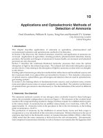
Fig. 11. X dependence of vertical force for Z=12 mm.
4.2 Equilibrium angle measurement
In addition to previous experiments, the mechanical behavior of a magnet which has the
ability to tilt over the superconductor in the Meissner state was also studied in this paper. In
the present experiment only one degree of freedom was permitted in the tilt angle of the
magnet (θ coordinate). The equilibrium angle of the permanent magnet over the cylindrical
superconductor was measured for different relative positions. The results can be used to
understand not only how the permanent magnet is repelled, but also how it turns when it is
released over a superconductor.


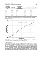
Fig. 12. Measurement system: 1 - Superconductor bulk, 2 - Permanent magnet, 3 -
Goniometer, 4 – Bearing (hidden), 5 – 3D table, 6 – Lab jack stand, 7 – Nitrogen vessel.

Foundations of Meissner Superconductor Magnet Mechanisms Engineering

165
A cylindrical permanent magnet (made of NdFeB with a coercivity of 875 kA/m and a
remanence of 1.29 T) was placed over the superconductor. Their dimensions were 6.3 mm in
diameter and 25.4 mm in length and it had a magnetization direction parallel to its axis of
revolution. A rigid plastic circular rod was fixed in the center of mass, perpendicular to the
axis of revolution. This rod was used as the shaft in a plastic bearing, which was lubricated
with oil. The whole bearing system was joined to a 3D displacement table. This arrangement
ensured it was possible to control the position of the permanent magnet with an accuracy of
0.1 mm, and the only permitted degree of freedom was the rotation around the Y axis.
Concentric to the bearing, a graduate goniometer measured the angle of rotation of the

magnet. The whole experiment design is shown in Fig 12.
Fig. 13 shows the comparison between the equilibrium angles measured and those
calculated by expression (19).


Fig. 13. Comparative graph between experimental and FEA calculus of the equilibrium
angle versus x position. Hight z was fixed at + 15 mm.
Again, there was a good agreement between the calculus made according to our model and
the experiments. These experiments were carried out in Zero Field cooling condition (ZFC),
and consequently there is no remanent magnetization.
5. Limits of application
The lower critical field, H
c1
, is one of the typical parameters of type II superconductors,
which has been experimentally being assessed from the magnetization changes from the
Meissner state slope to the reversible mixed-state behavior (Poole, 2007).
H
c1
is directly
related to the free energy of a flux line and contains information on essential mixed-state
parameters, such as the London penetration depth, λ
L
, and the Ginzburg–Landau
parameter, κ. Measurements of
H
c1
and, of course, of the upper critical field, H
c2
, therefore
provide a complete characterization of the mixed-state parameters of the superconductor.

Superconductivity – Theory and Applications

166
Differences between the predicted Meissner forces and the experimentally measured ones
indicate that a part of the sample is in the mixed-state. Establishing with precision the
instant when the differences begin will permit us to determine the
H
c1
mechanically.
Nevertheless, many other experimental techniques have been used to determine the state
transition; most of them based on some kind of d.c. or a.c. magnetic measurement, but also
on muon spin rotation (μSR) or magneto-optical techniques (Meilikhov & Shapiro, 1992).
The basic problem of magnetization measurements introduced by flux pinning lies in the
fact that the change of slope at the lower critical field is extremely small, since the first
penetrating flux lines are immediately pinned and change the overall magnetization
(
/
M
mV ) only marginally. Elaborate schemes of subtracting the measured moments
from an initial Meissner slope (Vandervoort et al., 1991; Webber et al., 1983) or experiments
providing us directly the derivative of magnetization (Hahn & Weber, 1983; Wacenoysky et
al., 1989; Weber et al., 1989) have been employed, SQUIDS have also been used to improve
the precision of these kind of means (Böhmer et al., 2007).
The method also determines the zone at the sample where transition from Meissner to
mixed state occurs.
For a position of the magnet with respect to the superconductor we define the Meissner
Efficacy as

ex

M
F
F

 (27)
where
F
ex
is the experimentally measured force and F
M
is the calculated force according with
the Meissner model cited above. For a certain position of the magnet a Meissner Efficacy
equal to one (
η =1) proves that the superconductor is completely in the Meissner state and
there is not any flux penetration. On the contrary, values lower than 1 indicate that a part of
the superconductor has flux penetration and is in the mixed-state.
The measurement for every position was made in zero field cooling conditions (ZFC). The
origin of coordinates was set at the center of the upper surface of the superconductor. The
reference point of the magnet was placed in the center of the lower surface of the magnet.
Therefore, the Z coordinate is the distance between the faces of the magnet and the
superconductor. X is the distance of the center of the magnet to the axis of the
superconductor cylinder (radial position). We have recorded the vertical forces for X = 0.0,
5.0, 10.0, 15.0, 17.5, 20.0, 22.5 and 25.0 ± 0.1 mm; at 4 different heights from the surface of the
superconductor: 12.0, 10.0, 8.0 and 6.0 ± 0.1 mm.
Fig. 14 shows the Meissner Efficacy versus the maximum of the surface current density
distribution
J
surf
for different positions.
We observe that for low values of the maximum surface current density, the Meissner

Efficacy is just 1.
From a certain value, the Meissner Efficacy decays linearly. From this data we can derive a
weighted mean value of
J
c1 surf
= 6452 ± 353 A/m for a polycrystalline YBa
2
Cu
3
O
7-x
sample at
77 K.
In Table 1
H
c1
values from different authors are shown for comparison. The values are those
obtained for the
H
c1
parallel to c-axis in monocrystalline samples. Our value for a
polycrystalline sample is of the same order of magnitude than the lowest monocrystalline
values.

Foundations of Meissner Superconductor Magnet Mechanisms Engineering

167

Fig. 14. Meissner Efficacy versus maximum Jsurf for different positions. The values obtained
for X=5.0, 10.0, 15.0 mm radial positions are similar to those obtained for the X=0.0 mm

values.
Now, if we use a value of
λ
L
=4500 Å, carried out from the literature (Geflbaux & Tazawa,
1998; Mayer & Schuster, 1993) we have a lower critical current density value of
Jc
1
= (1.43 ±
0.08)
×10
7
A/cm
2
. By using Eq. 2 we calculate Hc
1
= 3226 ± 176 A/m.


C. Bömer et al

(2007)
(monocr.)
Umewaza et
al (2007)
(monocr.)
Kaiser et al
(1991)
(monocr.)
Wu et al

(1990)
(monocr.)
Mechanical
method
(polycr.)
Results for H
c1
(A/m)
2900 ± 250
6000 ± 2300
4500 ± 450
3580
11000
4950
15518
3226 ± 176
Table 1. Comparison of the values found in different articles with that measured in this
paper. The values and relative errors have been obtained directly from graphs, at 77 K.
Available values for H  (a,b) and H
‖ (c) in monocrystals are shown. H ‖ (c) is always
greater than H  (a,b)
The uncertainty in the determination of
J
c1 surf
may be reduced by increasing the number of
series of measurements (or paths). Therefore, this is a method intrinsically more precise than
other common methods.
In fact, the values far from the Meissner state contribute to improve the accuracy of the
J
c1 surf

determination. The determination of the slopes of straight lines has a propagation of errors

Superconductivity – Theory and Applications

168
more convenient than that in the case of the measurement of a change in the slope of the
tangents to a curve. Other methods, therefore, would require high precision measurements
to obtain a reasonable error for Hc1.
This results are in according to the border and thickness effects and border magnetization
that have been already described by other authors in an uniform magnetic field ( Brandt,
2000; Morozov et al., 1996; Li et al., 2004; Schmidt et al., 1997):
6. Example of application - permanent magnet over a superconducting torus
We calculate the torque exerted between a superconducting torus and a permanent magnet
by using this model. We find that there is a flip effect on the stablest direction of the magnet
depending on its position. This could be easily used as a digital detector for proximity.
We consider a full superconducting torus and a cylindrical permanent NdFeB magnet over
the superconductor axis (Z axis). In figure 15 we can observe the geometrical configuration
of both components. Every calculation is referenced with respect of a Cartesian coordinate
system placed in the center of mass of the torus which Z axis is coincident with the axis of
the torus.


Fig. 15. Permanent magnet over a toroidal superconductor set-up. The dimensions are: L
PM
-
length of the cylindrical permanent magnet, Ø
PM
– diameter of the cylindrical permanent
magnet, R

INT
– Inner radius of the torus, Ø
SECTION
– Diameter of the circular section of the
torus. z is the vertical coordinate of the center of the magnet and θ is the angle between the
axis of the magnet and the vertical Z axis.
The superconducting torus has an internal radius R
INT
= 6 mm and a diameter of the section
Ø
SECTION
= 10 mm. The cylindrical permanent magnet has a length L
PM
= 5 mm and a
diameter Ø
PM
= 5 mm. When calculating the magnetic field generated by the magnet we
define its magnetic properties as: Coercive magnetic field H
COERCIVITY
= 875 kA/m and
remanent magnetic flux density B
REMANENT
= 1.18 T. We assume that the direction of
magnetization of the permanent magnet coincides with its axis of revolution.
The variables θ and z are the coordinates we modify in order to analyze the mechanical
behavior of the magnet over the superconductor. z is the distance along the Z axis between

Foundations of Meissner Superconductor Magnet Mechanisms Engineering

169

the center of mass of the torus and the one of the cylindrical permanent magnet. θ is the
angle between the axis of the magnet and the vertical Z axis.
The equilibrium angle (θ
eq
) as a function of z can be determined as follows. For a certain z
we calculate the Y component of the torque (M
y
) exerted on the magnet by the
superconductor as a function of θ and we find the equilibrium angle as the value for which
M
y
(θ
eq
)=0. The sign of the slope dM
y
/dθ at that point determines the stability or instability
of the equilibrium point.


Fig. 16. M
y
applied to the permanent magnet by the superconductor as a function of θ for z=
0, 3, 6, 9, 12 and 15 mm.
In figure 16 the torque (M
y
) exerted on the magnet by the superconductor as a function of θ
is shown for z = 0, 3, 6, 9, 12 and 15 mm. The maximum values for the torque exerted to the
permanent magnet appear at θ = 45º and θ = 135º for every z. The remarkable fact is that the
sign suddenly changes when moving from z = 3 mm to z = 6 mm. The equilibrium points
are always at θ = 0º and θ = 90º, but θ = 0º is a stable equilibrium point for z = 0 mm and z =

3 mm, while it is unstable for the rest of the positions. On the other hand θ = 90º is unstable
for z = 0 mm and z = 3 mm, but it is stable for the rest of the positions. That means that if
you approach a magnet along the Z axis and it is able to rotate, it will be perpendicular to
the Z axis while it is at z

≥ 6 mm, but it will suddenly rotate to be parallel to the Z axis when
you pass from z = 6 to z ≤ 3.
In figure 17 the variation of the torque at θ = 45º as a function of z. The torque changes its
sign between z =3 mm and z =4 mm.
Finally, figure 18 shows the stable equilibrium angle as a function of z. It is evident that, at a
certain position between z =+ 3 and z =+ 4 mm we found that the stable equilibrium angle
switches from a vertical orientation of the magnet to an horizontal one describing the flip
effect claimed in this work.
Therefore, it can be concluded that if you approach a magnet along the Z axis and it is able
to rotate, it will be perpendicular to the Z axis while it is at a certain distance (z ≥ 4 mm in

Superconductivity – Theory and Applications

170
our example) and it will change to be parallel to the Z axis for closer positions (z ≤ 3 mm in
our example). As the equilibrium angle does not depend on the magnetic moment, the
magnet can be much smaller. As a flip in the orientation of a permanent magnet can be
easily instrumented, this effect can be easily used as a binary detector for proximity.


Fig. 17. Torque M
y
exerted on the magnet for θ = 45º as a function of z.

Fig. 18. Stable equilibrium angle (θ
eq
) as a function of z.
7. Conclusion
Magnet-superconductor forces both in Meissner and mixed states can be calculated with the
accuracy required to engineer useful levitating devices.
The implementation of a local differential expression in a finite elements program opens
new perspectives to the use of magnet-superconductor devices for engineering. This can be

Foundations of Meissner Superconductor Magnet Mechanisms Engineering

171
used to calculate forces whatever the size, shape and geometry of the system, for both
permanent magnets and electromagnets.
Accuracy and convergence, in addition to the experimental verification for different cases
have been tested. There is a good agreement between experimental results and calculation,
even with very low-cost computing resources involved.
Moreover, the expression can be used to determine the point when the mixed state arises in
a superconductor piece.
8. References
Alario, M.A. & Vicent, J.L. (1991). Superconductividad, 1st ed. (EUDEMA, Madrid, 1991).
Arkadiev, V. (1947). A floating magnet.
Nature 160, 330 (1947).
Bednorz, J.G. & Müller, K.A. (1986). Possible highT c superconductivity in the Ba- La- Cu- O

system. Zeitschrift Für Physik B Condensed Matte.r 64, 189–193 (1986).
Böhmer, C.; Brandstatter, G. & Weber, H. (2007). The lower critical field of high-temperature

superconductors. Supercond. Sci. Techn., 10 (2007) A1-A10
Brandt, E.H. (2000). Superconductors in realistic

g
eometries:
g
eometric ed
g
e barrier versus
pinning.
Physica C, 332 (2000) 99-107
Buchhold, T.A. (1960). Applications of superconductivity.
Scientific American 3, 74 (1960).
Cansiz, A.; Hull, J.R. & Gundogdu O. (2005). Translational and rotational d
y
namic anal
y
sis
of a superconducting levitation system.
Supercond. Sci. Technol. 18, 990 (2005).
Diez-Jimenez E. et al
. (2010). Finite element algorithm for solving supercondcutin
g
Meissner

repulsion forces. Icec 23 - Icmc 2010 (Wroclaw (Poland), 2010).
Early, E.A.; Seaman, C.L.; Yang, K.N. & Maple
, M.B. (1988) American Journal Of Physics 56,

617 (1988).
Geflbaux, X. & Tazawa
, M. (1998). Étude de la variation de la longueur de London entre 5 et

70 K , dans un film très mince d ’ YBaCuOç6 , par spectromérie dans I ’ infrarou
g
e

lointain ; comparaison avec NbN. C.R. de l’Academie Sciences. Fasc. B, 324 (1998) 389-
397
Giaro, K.; Gorzkowski, W. & Motylewski
, T. (1990). A correct description of the interaction

between a magnetic moment and its image. Physica C 168, 479-481 (1990).
Gijutsucho, K. (2001)
Patent JP2001004652-A, (2001) Japan
Hahn, P. & Weber
, H.W. (1983). Automatic device for ma
g
netization measurements on
superconductors.
Cryogenics, 23 (1983) 87-90
Hellman F. et al
. (1988). Levitation of a magnet over a flat type II superconductor. Journal O
f
applied Physics 63, 447 (1988).
Hull, J.R. & Cansiz
, A. (1999). Vertical and lateral forces between a permanent ma
g
net and a
high-temperature superconductor.
Journal Of Applied Physics 86, (1999).
Hull, J.R. (2000). Superconducting bearings.
Supercond. Sci. Techn., 13 (2000) R1–R15

J
ackson, J.D. (1975) Classical Electrodynamics (John Wiley & Sons, New York, 1975).
Kaiser, D.L. & Swartzendruber
, L.J. (1991). Lower critical field measurements in YBACUO
single cristals.
Proc. Adv. in mat. sci. & appl. of HTSC (1991)
Li, Q.; Suenaga, M. & Ye, Z. (2004). Crossover of thickness dependence of critical current
density J(c)(T,H) in YBa2Cu3O7-delta thick films. App.
Physics Lett. 84 (2004) 3528-
3530
Lin, Q. (2006). Theoretical development of the ima
g
e method for a
g
eneral ma
g
netic source

Superconductivity – Theory and Applications

172
in the presence of a superconducting sphere or a long superconducting cylinder.
Physical Review B 74, 24510 (2006).
Mayer, B. & Schuster, S. (1993). Magnetic-field dependence of the critical current in
yba2cu3o7-delta bicrystal grain-boundary junctions.
App. Physics Lett. 63 (1993)

783-785
Meilikhov, E. & Shapiro, V.G. (1992). Critical fields of the htsc superconductors.
Su

p
ercond.

Sci. Techn., 5 (1992) S391-S394
Moon, F.C. (1994).
Superconducting Levitation (John Wiley & Sons, New York, 1994).
Morozov, N. & Zeldov, E. (1996). Negative local permeability in Bi2Sr2CaCu2O8 crystals.
Phys. Rev. Lett. 76 (1996) 138-141
Perez-Diaz, J.L. & Garcia-Prada, J.C. (2007). Finite-size-induced stabilit
y
of a permanent

magnet levitating over a superconductor in the Meissner state. A
pp
lied Ph
y
sics

Letters 91, 142503 (2007).
Perez-Diaz, J.L. & Garcia-Prada, J.C. (2007). Interpretation of the method of ima
g
es in

estimating superconducting levitation. Physica C 467, 141-144 (2007).
Perez-Diaz, J.L.; Garcia-Prada, J.C. & Diaz-Garcia, J.A. (2008). Universal Model for

Superconductor-Magnet Forces in the Static Limit. I.R.E.M.E. 2, (2008).
Poole, C.P. (2007)
Superconductivity, 2nd ed.,AP, Elsevier, 2007
Schmidt, B.; Morozov, N. & Zeldov, E. (1997). Angular dependence of the first-order vortex-

lattice phase transition in Bi2Sr2CaCu2O8.
Phys. Rev. B, 55 (1997) R8705-R8708
Simon
, I. (1953). Forces acting on superconductors in magnetic fields. Journal O
f
A
pp
lie
d
Physics 24, 19 (1953).
Umezawa, A. & Crabtree, A. (1998). Anisotrop
y
of the lowr critical field, ma
g
netic
penetration depth, and equilibrium shielding current y single-crystal YBACUO.
Physical Review B. 38, (1998).
Vandervoort, K.G.; Welp, U. & Kessler, J.E. (1991). Ma
g
netic measurements of the upper and

lower critical fields of oxygen-deficient yba2cu3o7-delta single-crystals. Ph
y
s. Rev.

B, 43 (1991) 13042-13048
Wacenovsky, M.; Weber, H.; Hyun, O.B. (1989). Magnetization of grain-aligned hoba2cu3o7-
delta.
Physica C, 162 (1989) 1629-1630
Weber, H.W.; Seidl, E. & Laa, C. (1991). Anisotropy effects in superconducting niobium.

Phys. Rev. B, 44 (1991) 7585-7600
Wu, D.H. & Sridhar, S. (1990). Pinnin
g
forces and lower critical fields in YBACUO cr
y
stals:
temperature dependence and anisotropy.
Phys. Rev. Lett. 65 (1990) 2074-2077
Yang, Y. & Zheng
, X. (2007). Method for solution of the interaction between superconductor

and permanent magnet. Journal Of Applied Physics 101, 113922 (2007).

9
Properties of Macroscopic Quantum
Effects and Dynamic Natures of
Electrons in Superconductors
Pang Xiao-feng
Institute of Life Science and Technology, University of
Electronic Science and Technology of China, Chengdu,
International Centre for Materials Physics,
Chinese Academy of Science, Shenyang,
China
1. Introduction
So-called macroscopic quantum effects(MQE) refer to a quantum phenomenon that occurs
on a macroscopic scale. Such effects are obviously different from the microscopic quantum
effects at the microscopic scale as described by quantum mechanics. It has been
experimentally demonstrated [1-17] that macroscopic quantum effects are the phenomena
that have occurred in superconductors. Superconductivity is a physical phenomenon in
which the resistance of a material suddenly vanishes when its temperature is lower than a

certain value, Tc, which is referred to as the critical temperature of superconducting
materials. Modern theories [18-21] tell us that superconductivity arises from the irresistible
motion of superconductive electrons. In such a case we want to know “How the
macroscopic quantum effect is formed? What are its essences? What are the properties and
rules of motion of superconductive electrons in superconductor?” and, as well, the answers
to other key questions. Up to now these problems have not been studied systematically. We
will study these problems in this chapter.
2. Experimental observation of property of macroscopic quantum effects in
superconductor
(1) Superconductivity of material. As is known, superconductors can be pure elements,
compounds or alloys. To date, more than 30 single elements, and up to a hundred alloys and
compounds, have been found to possess the characteristics [1-17] of superconductors.
When
c
TT≤ , any electric current in a superconductor will flow forever without being
damped. Such a phenomenon is referred to as perfect conductivity. Moreover, it was
observed through experiments that, when a material is in the superconducting state, any
magnetic flux in the material would be completely repelled resulting in zero magnetic fields
inside the superconducting material, and similarly, a magnetic flux applied by an external
magnetic field can also not penetrate into superconducting materials. Such a phenomenon is

Superconductivity – Theory and Applications

174
called the perfect anti-magnetism or Maissner effect. Meanwhile, there are also other
features associated with superconductivity, which are not present here
How can this phenomenon be explained? After more than 40 years’ effort, Bardeen, Cooper
and Schreiffier proposed the new idea of Cooper pairs of electrons and established the
microscopic theory of superconductivity at low temperatures, the BCS theory [18-21],in
1957, on the basis of the mechanism of the electron-phonon interaction proposed by Frohlich

[22-23]. According to this theory, electrons with opposite momenta and antiparallel spins
form pairs when their attraction, due to the electron and phonon interaction in these
materials, overcomes the Coulomb repulsion between them. The so-called Cooper pairs are
condensed to a minimum energy state, resulting in quantum states, which are highly
ordered and coherent over the long range, and in which there is essentially no energy
exchange between the electron pairs and lattice. Thus, the electron pairs are no longer
scattered by the lattice but flow freely resulting in superconductivity. The electron pairs in a
superconductive state are somewhat similar to a diatomic molecule but are not as tightly
bound as a molecule. The size of an electron pair, which gives the coherent length, is
approximately 10
−4
cm. A simple calculation shows that there can be up to 10
6
electron pairs
in a sphere of 10
−4
cm in diameter. There must be mutual overlap and correlation when so
many electron pairs are brought together. Therefore, perturbation to any of the electron
pairs would certainly affect all others. Thus, various macroscopic quantum effects can be
expected in a material with such coherent and long range ordered states. Magnetic flux
quantization, vortex structure in the type-II superconductors, and Josephson effect [24-26] in
superconductive junctions are only some examples of the phenomena of macroscopic
quantum mechanics.
(2) The magnetic flux structures in superconductor. Consider a superconductive ring.
Assume that a magnetic field is applied at T >Tc, then the magnetic flux lines
0
φ
produced
by the external field pass through and penetrate into the body of the ring. We now lower the
temperature to a value below Tc, and then remove the external magnetic field. The magnetic

induction inside the body of circular ring equals zero (
B


= 0) because the ring is in the
superconductive state and the magnetic field produced by the superconductive current
cancels the magnetic field, which was within the ring. However, part of the magnetic fluxes
in the hole of the ring remain because the induced current is in the ring vanishes. This
residual magnetic flux is referred to as “the frozen magnetic flux”. It has been observed
experimentally, that the frozen magnetic flux is discrete, or quantized. Using the
macroscopic quantum wave function in the theory of superconductivity, it can be shown
that the magnetic flux is established by
0
' nΦ=
φ
(n=0,1,2,…), where
0
φ
=hc/2e=2.07×10
-15

Wb is the flux quantum, representing the flux of one magnetic flux line. This means that the
magnetic fluxes passing through the hole of the ring can only be multiples of
0
φ
[1-12]. In
other words, the magnetic field lines are discrete. We ask, “What does this imply?” If the
magnetic flux of the applied magnetic field is exactly n, then the magnetic flux through the
hole is n
0

φ
, which is not difficult to understand. However, what is the magnetic flux
through the hole if the applied magnetic field is (n+1/4)
0
φ
? According to the above, the
magnetic flux cannot be (n+1/4)
0
φ
. In fact, it should be n
0
φ
. Similarly, if the applied
magnetic field is (n+3/4)
0
φ
and the magnetic flux passing through the hole is not
(n+3/4)
0
φ
, but rather (n+1)
0
φ
, therefore the magnetic fluxes passing through the hole of
the circular ring are always quantized.
Properties of Macroscopic Quantum Effects
and Dynamic Natures of Electrons in Superconductors

175
An experiment conducted in 1961 surely proves this to be so, indicating that the

magnetic flux does exhibit discrete or quantized characteristics on a macroscopic scale.
The above experiment was the first demonstration of the macroscopic quantum effect.
Based on quantization of the magnetic flux, we can build a “quantum magnetometer”
which can be used to measure weak magnetic fields with a sensitivity of 3×10
-7
Oersted.
A slight modification of this device would allow us to measure electric current as low as
2.5×10
-9
A.
(3) Quantization of magnetic-flux lines in type-II superconductors. The superconductors
discussed above are referred to as type-I superconductors. This type of superconductor
exhibits a perfect Maissner effect when the external applied field is higher than a critical
magnetic value
c
H

. There exists other types of materials such as the NbTi alloy and Nb
3
Sn
compounds in which the magnetic field partially penetrates inside the material when the
external field
H

is greater than the lower critical magnetic field
1c
H


, but less than the

upper critical field
2c
H


[1-7]. This kind of superconductor is classified as type-II
superconductors and is characterized by a Ginzburg-Landau parameter greater than 1/2.
Studies using the Bitter method showed that the penetration of a magnetic field results in
some small regions changing from superconductive to normal state. These small regions in
normal state are of cylindrical shape and regularly arranged in the superconductor, as
shown in Fig.1. Each cylindrical region is called a vortex (or magnetic field line)[1-12]. The
vortex lines are similar to the vortex structure formed in a turbulent flow of fluid. Both
theoretical analysis and experimental measurements have shown that the magnetic flux
associated with one vortex is exactly equal to one magnetic flux quantum
0
φ
, when the
applied field
1c
HH≥

, the magnetic field penetrates into the superconductor in the form of
vortex lines, increased one by one. For an ideal type-II superconductor, stable vortices are
distributed in triagonal pattern, and the superconducting current and magnetic field
distributions are also shown in Fig. 1. For other, non-ideal type-II superconductors, the
triagonal pattern of distribution can be also observed in small local regions, even though its
overall distribution is disordered. It is evident that the vortex-line structure is quantized and
this has been verified by many experiments and can be considered a result of the
quantization of magnetic flux. Furthermore, it is possible to determine the energy of each
vortex line and the interaction energy between the vortex lines. Parallel magnetic field lines

are found to repel each other while anti-parallel magnetic lines attract each other.
(4) The Josephson phenomena in superconductivity junctions [24-26]. As it is known in
quantum mechanics, microscopic particles, such as electrons, have a wave property and that
can penetrate through a potential barrier. For example, if two pieces of metal are separated
by an insulator of width of tens of angstroms, an electron can tunnel through the insulator
and travel from one metal to the other. If voltage is applied across the insulator, a tunnel
current can be produced. This phenomenon is referred to as a tunneling effect. If two
superconductors replace the two pieces of metal in the above experiment, a tunneling
current can also occur when the thickness of the dielectric is reduced to about 30
0
A .
However, this effect is fundamentally different from the tunneling effect discussed above in
quantum mechanics and is referred to as the Josephson effect.
Evidently, this is due to the long-range coherent effect of the superconductive electron pairs.
Experimentally, it was demonstrated that such an effect could be produced via many types

Superconductivity – Theory and Applications

176
of junctions involving a superconductor, such as superconductor-metal-superconductor
junctions, superconductor-insulator- superconductor junctions, and superconductor bridges.
These junctions can be considered as superconductors with a weak link. On the one hand,
they have properties of bulk superconductors, for example, they are capable of carrying
certain superconducting currents. On the other hand, these junctions possess unique
properties, which a bulk superconductor does not. Some of these properties are summarized
in the following.
(A) When a direct current (dc) passing through a superconductive junction is smaller than a
critical value Ic, the voltage across the junction does not change with the current. The critical
current Ic can range from a few tens of μA to a few tens of mA.
(B) If a constant voltage is applied across the junction and the current passing through the

junction is greater than Ic, a high frequency sinusoidal superconducting current occurs in
the junction. The frequency is given by υ=2eV/h, in the microwave and far-infrared regions
of (5-1000)×10
9
Hz. The junction radiates a coherent electromagnetic wave with the same
frequency. This phenomenon can be explained as follows: The constant voltage applied
across the junction produces an alternating Josephson current that, in turn, generates an
electromagnetic wave of frequency, υ. The wave propagates along the planes of the junction.
When the wave reaches the surface of the junction (the interface between the junction and its
surrounding), part of the electromagnetic wave is reflected from the interface and the rest is
radiated, resulting in the radiation of the coherent electromagnetic wave. The power of
radiation depends on the compatibility between the junction and its surrounding.
(C) When an external magnetic field is applied over the junction, the maximum dc current,
Ice , is reduced due to the effect of the magnetic field. Furthermore, I
c
changes periodically
as the magnetic field increases. The
c
IH− curve resembles the distribution of light intensity
in the Fraunhofer diffraction experiment , and the latter is shown in Fig. 2. This
phenomenon is called quantum diffraction of the superconductivity junction.


Fig. 1. Current and magnetic field distributionseffect in in a type-II superconductor.
Properties of Macroscopic Quantum Effects
and Dynamic Natures of Electrons in Superconductors

177

Fig. 2. Quantum diffractionsuperconductor junction

(D) When a junction is exposed to a microwave of frequency, υ, and if the voltage applied
across the junction is varied, it can be seen that the dc current passing through the junction
increases suddenly at certain discrete values of electric potential. Thus, a series of steps
appear on the dc I − V curve, and the voltage at a given step is related to the frequency of
the microwave radiation by nυ=2eVn/h(n=0,1,2,3…). More than 500 steps have been
observed in experiments.
Josephson first derived these phenomena theoretically and each was experimentally verified
subsequently. All these phenomena are, therefore, called Josephson effects [24-26]. In
particular, (1) and (3) are referred to as dc Josephson effects while (2) and (4) are referred to
as ac Josephson effects. Evidently, Josephson effects are macroscopic quantum effects, which
can be explained well by the macroscopic quantum wave function. If we consider a
superconducting junction as a weakly linked superconductor, the wave functions of the
superconducting electron pairs in the superconductors on both sides of the junction are
correlated due to a definite difference in their phase angles. This results in a preferred
direction for the drifting of the superconducting electron pairs, and a dc Josephson current
is developed in this direction. If a magnetic field is applied in the plane of the junction, the
magnetic field produces a gradient of phase difference, which makes the maximum current
oscillate along with the magnetic field, and the radiation of the electromagnetic wave occur.
If a voltage is applied across the junction, the phase difference will vary with time and
results in the Josephson effect. In view of this, the change in the phase difference of the
wave functions of superconducting electrons plays an important role in Josephson effect,
which will be discussed in more detail in the next section.
The discovery of the Josephson effect opened the door for a wide range of applications of
superconductor theory. Properties of superconductors have been explored to produce
superconducting quantum interferometer–magnetometer, sensitive ammeter, voltmeter,
electromagnetic wave generator, detector, frequency-mixer, and so on.

Superconductivity – Theory and Applications

178

3. The properties of boson condensation and spontaneous coherence of
macroscopic quantum effects
3.1 A nonlinear theoretical model of theoretical description of macroscopic quantum
effects
From the above studies we know that the macroscopic quantum effect is obviously different
from the microscopic quantum effect, the former having been observed for physical
quantities, such as, resistance, magnetic flux, vortex line, and voltage, etc.
In the latter, the physical quantities, depicting microscopic particles, such as energy,
momentum, and angular momentum, are quantized. Thus it is reasonable to believe that the
fundamental nature and the rules governing these effects are different.
We know that the microscopic quantum effect is described by quantum mechanics.
However, the question remains relative to the definition of what are the mechanisms of
macroscopic quantum effects? How can these effects be properly described?
What are the states of microscopic particles in the systems occurring related to macroscopic
quantum effects? In other words, what are the earth essences and the nature of macroscopic
quantum states? These questions apparently need to be addressed.
We know that materials are composed of a great number of microscopic particles, such as
atoms, electrons, nuclei, and so on, which exhibit quantum features. We can then infer, or
assume, that the macroscopic quantum effect results from the collective motion and
excitation of these particles under certain conditions such as, extremely low temperatures,
high pressure or high density among others. Under such conditions, a huge number of
microscopic particles pair with each other condense in low-energy state, resulting in a
highly ordered and long-range coherent. In such a highly ordered state, the collective
motion of a large number of particles is the same as the motion of “single particles”, and
since the latter is quantized, the collective motion of the many particle system gives rise to a
macroscopic quantum effect. Thus, the condensation of the particles and their coherent state
play an essential role in the macroscopic quantum effect.
What is the concept of condensation? On a macroscopic scale, the process of transforming
gas into liquid, as well as that of changing vapor into water, is called condensation. This,
however, represents a change in the state of molecular positions, and is referred to as a

condensation of positions. The phase transition from a gaseous state to a liquid state is a first
order transition in which the volume of the system changes and the latent heat is produced,
but the thermodynamic quantities of the systems are continuous and have no singularities.
The word condensation, in the context of macroscopic quantum effects has its’ special
meaning. The condensation concept being discussed here is similar to the phase transition
from gas to liquid, in the sense that the pressure depends only on temperature, but not on
the volume noted during the process, thus, it is essentially different from the above, first-
order phase transition. Therefore, it is fundamentally different from the first-order phase
transition such as that from vapor to water. It is not the condensation of particles into a
high-density material in normal space. On the contrary, it is the condensation of particles to
a single energy state or to a low energy state with a constant or zero momentum. It is thus
also called a condensation of momentum. This differs from a first-order phase transition and
theoretically it should be classified as a third order phase transition, even though it is really
a second order phase transition, because it is related to the discontinuity of the third
derivative of a thermodynamic function. Discontinuities can be clearly observed in
measured specific heat, magnetic susceptibility of certain systems when condensation
Properties of Macroscopic Quantum Effects
and Dynamic Natures of Electrons in Superconductors

179
occurs. The phenomenon results from a spontaneous breaking of symmetries of the system
due to nonlinear interaction within the system under some special conditions such as,
extremely low temperatures and high pressures. Different systems have different critical
temperatures of condensation. For example, the condensation temperature of a
superconductor is its critical temperature
c
T , and from previous discussions[27-32].
From the above discussions on the properties of superconductors, and others we know that,
even though the microscopic particles involved can be either Bosons or Fermions, those
being actually condensed, are either Bosons or quasi-Bosons, since Fermions are bound as

pairs. For this reason, the condensation is referred to as Bose-Einstein condensation[33-36]
since Bosons obey the Bose-Einstein statistics. Properties of Bosons are different from those
of Fermions as they do not follow the Pauli exclusion principle, and there is no limit to the
number of particles occupying the same energy levels. At finite temperatures, Bosons can
distribute in many energy states and each state can be occupied by one or more particles,
and some states may not be occupied at all. Due to the statistical attractions between Bosons
in the phase space (consisting of generalized coordinates and momentum), groups of Bosons
tend to occupy one quantum energy state under certain conditions. Then when the
temperature of the system falls below a critical value, the majority or all Bosons condense to
the same energy level (e.g. the ground state), resulting in a Bose condensation and a series of
interesting macroscopic quantum effects. Different macroscopic quantum phenomena are
observed because of differences in the fundamental properties of the constituting particles
and their interactions in different systems.
In the highly ordered state of the phenomena, the behavior of each condensed particle is
closely related to the properties of the systems. In this case, the wave function
i
e
f
θ
φ= or
i
e
θ
φ
=
ρ
of the macroscopic state[33-35], is also the wave function of an individual
condensed particle. The macroscopic wave function is also called the order parameter of the
condensed state. This term was used to describe the superconductive states in the study of
these macroscopic quantum effects. The essential features and fundamental properties of

macroscopic quantum effect are given by the macroscopic wave function
φ and it can be
further shown that the macroscopic quantum states, such as the superconductive states are
coherent and are Bose condensed states formed through second-order phase transitions after
the symmetry of the system is broken due to nonlinear interaction in the system.
In the absence of any externally applied field, the Hamiltonian of a given macroscopic
quantum system can be represented by the macroscopic wave function
φ and written as

224
1
H' [ ]
2
Hdx dx==−∇
φ
−α
φ
+λ
φ

(1)
Here H’=H
presents the Hamiltonian density function of the system, the unit system in
which m=h=c=1 is used here for convenience. If an externally applied electromagnetic field
does exist, the Hamiltonian given above should be replaced by

2
2
24
*

1H
HH' ieA
28
dx dx




==−∇−φ−αφ+λφ+
π








(2)
or, equivalently

Superconductivity – Theory and Applications

180
ji
2
24
*
jj ji
11

HH' (ieA) F.F
24
dx dx


==−∂−φ−αφ+λφ+






where
ji j i t
FAA
j
=∂ −∂ is the covariant field intensity,
H= A∇×



is the magnetic field
intensity, e is the charge of an electron, and e*=2e,
A

is the vector potential of the
electromagnetic field,
α and λ can be said to be some of the interaction constants. The
above Hamiltonians in Eqs.(1) and (2) have been used in studying superconductivity by
many scientists, including Jacobs de Gennes [37], Saint-Jams [38], Kivshar [39-40], Bullough

[41-42], Huepe [43], Sonin [44], Davydov [45], et al., and they can be also derived from the
free energy expression of a superconductive system given by Landau et al [46-47]. As a
matter of fact, the Lagrangian function of a superconducting system can be obtained from
the well-known Ginzberg-Landau (GL) equation [47-54] using the Lagrangian method, and
the Hamiltonian function of a system can then be derived using the Lagrangian approach.
The results, of course, are the same as Eqs. (1) and (2). Evidently, the Hamiltonian operator
corresponding to Eqs. (1) and (2) represents a nonlinear function of the wave function of a
particle, and the nonlinear interaction is caused by the electron-phonon interaction and due
to the vibration of the lattice in BCS theory in the superconductors. Therefore, it truly exists.
Evidently, the Hamiltonians of the systems are exactly different from those in quantum
mechanics, and a nonlinear interaction related to the state of the particles is involved in Eqs.
(1) –(2). Hence, we can expect that the states of particles depicted by the Hamiltonian also
differ from those in quantum mechanics, and the Hamiltonian can describe the features of
macroscopic quantum states including superconducting states. These problems are to be
treated in the following pages. Evidently, the Hamiltonians in Eqs. (1) and (2) possess the U
(1) symmetry. That is, they remain unchanged while undergoing the following
transformation:
(,) (,) (,)
j
iQ
rt rt e rt
−θ
′
φ→φ = φ



where
j
Q is the charge of the particle，θ is a phase and, in the case of one dimension, each

term in the Hamiltonian in Eq. (1) or Eq. (2) contains the product of the ( , )
j
xts
φ
, then we
can obtain:
12
()
'' '
12 12
(,) (,) (,) (,) (,) (,)
n
iQ Q Q
nn
xt xt xt e xt xt xt
− + +⋅⋅⋅+ θ
φφ φ = φφ φ
Since charge is invariant under the transformation and neutrality is required for the
Hamiltonian, there must be (Q
1
+ Q
2
+ · · · + Q
n
) = 0 in such a case. Furthermore, since θ is
independent of x, it is necessary that
j
iQ
jj
e

−θ
∇
φ
→∇
φ
. Thus each term in the Hamiltonian in
Eqs. (1) is invariant under the above transformation, or it possesses the U(1) symmetry[16-17].
If we rewrite Eq. (1) as the following

224
eff eff
1
H' =- ( ) U ( ),U ( )
2
∇
φ
+
φφ
=−α
φ
+λ
φ
(3)
We can see that the effective potential energy, ( )
eff
U
φ
, in Eq. (3) has two sets of extrema,
0
/2φ=±α λ

and
0
φ
=0, but the minimum is located at

0
/2 0 0 ,φ=±α λ= φ (4)
Properties of Macroscopic Quantum Effects
and Dynamic Natures of Electrons in Superconductors

181
rather than at
0
φ
=0 . This means that the energy at
0
/2
φ
=± α λ is lower than that at
0
φ
=0.
Therefore,
0
φ
=0 corresponds to the normal ground state, while
0
/2
φ
=± α λ is the ground

state of the macroscopic quantum systems .
In this case the macroscopic quantum state is the stable state of the system. This shows that
the Hamiltonian of a normal state differs from that of the macroscopic quantum state, in
which the two ground states satisfy
00 00φ≠−φ
under the transformation,
φ
→−
φ
.
That is, they no longer have the U(1) symmetry. In other words
，the symmetry of the
ground states has been destroyed. The reason for this is evidently due to the nonlinear term
4
λ
φ
in the Hamiltonian of the system. Therefore, this phenomenon is referred to as a
spontaneous breakdown of symmetry. According to Landau’s theory of phase
transition,
the system undergoes a second-order phase transition in such a case, and the normal ground
state
0
φ
==0 is changed to the macroscopic quantum ground state
0
/2
φ
=± α λ . Proof will
be presented in the following example .
In order to make the expectation value in a new ground state zero in the macroscopic

quantum state, the following transformation [16-17] is done:

'
0
φ
=
φ
+
φ
(5)
so that

0'0φ =0 (6)
After this transformation, the Hamiltonian density of the system becomes

2
22 3 3 424
000000
1
H'( + ) (6 ) 4 (4 2 )
2
φφ
=∇
φ
+λ
φ
−α
φ
+λ
φφ

+λ
φ
−α
φφ
+λ
φ
−α
φ
+λ
φ
(7)
Inserting Eq. (4) into Eq. (7), we have
2
00 0
42 0
φ
λ
φ
−α
φ
= .
Consider now the expectation value of the variation
H'/
δδφ
in the ground state, i.e.
'
000
Hδ
=
δφ

, then from Eq. (1), we get

23
'
000- 2400
Hδ
=∇
φ
+α
φ
−λ
φ
=
δφ
(8)
After the transformation Eq. (6), it becomes

22 2 3 2
000 0 0
(4 2 ) 12 0 0 4 0 0 (2 12 ) 0 0 0∇
φ
+λ
φ
−α
φ
+λ
φφ
+λ
φ
−α− λ

φφ
= (9)
where the terms
3
00φ
and 00
φ
are both zero, but the fluctuation
2
0
12 0 0λφ φ
of the
ground state is not zero. However, for a homogeneous system, at T=0K, the term
2
00φ is
very small and can be neglected.
Then Eq. (9) can be written as

22
00 0
-(42)0∇φ − λφ − αφ =
(10)

Superconductivity – Theory and Applications

182
Obviously, two sets of solutions,
0
0
φ

= , and
0
/2
φ
=± α λ , can be obtained from the
above equation, but we can demonstrate that the former is unstable, and that the latter is
stable.
If the displacement is very small, i.e.
'
0000
φ
→
φ
+δ
φ
=
φ
, then the equation satisfied by the
fluctuation
0
δ
φ
is relative to the normal ground state
0
0
φ
= and is

2
00

20∇δφ − αδφ =
(11)
Its’ solution attenuates exponentially indicating that the ground state,
0
0
φ
= is unstable.
On the other hand, the equation satisfied by the fluctuation
0
δ
φ
, relative to the ground
state
0
/2φ=±α λ is
2
00
20∇δφ + αδφ = . Its’ solution,
0
δ
φ
, is an oscillatory function and
thus the macroscopic quantum state ground state
0
/2
φ
=± α λ is stable. Further
calculations show that the energy of the macroscopic quantum state ground state is lower
than that of the normal state by
2

0
/4 0ε=−α λ< .Therefore, the ground state of the
normal phase and that of the macroscopic quantum phase are separated by an energy gap
of
2
/(4 )αλso then, at T=0K, all particles can condense to the ground state of the
macroscopic quantum phase rather than filling the ground state of the normal phase.
Based on this energy gap, we can conclude that the specific heat of the macroscopic
quantum systems has an exponential dependence on the temperature, and the critical
temperature is given by:
cp
T=1.14 exp[ 1/(3 / )N(0)]ω−λα [16-17]. This is a feature of the
second-order phase transition. The results are in agreement with those of the BCS theory
of superconductivity.
Therefore, the transition from the state
0
0
φ
= to the state
0
/2
φ
=± α λ and the
corresponding condensation of particles are second-order phase transitions. This is
obviously the results of a spontaneous breakdown of symmetry due to the nonlinear
interaction,
4
λ
φ
.

In the presence of an electromagnetic field with a vector potential
A


, the Hamiltonian of the
systems is given by Eq. (2). It still possesses the U (1) symmetry.Since the existence of the
nonlinear terms in Eq. (2) has been demonstrated, a spontaneous breakdown of symmetry
can be expected. Now consider the following transformation:

12 102
11
(x) [ (x) i (x)] [ (x) +i (x)]
22
φ= φ+φ → φ+φφ (12)
Since
i
000
φ
= under this transformation, then the equation (2) becomes
2
222 222
ij ji 2 1 1 0 2 i 0i 2
22 22 22
21 12i 0 1 0 2 011 2
222 2 2 2
12 0 0 1 0 0
111(e*)
H' ( A A ) ( ) ( ) [( ) ]A e * A
4222
11

e*( )A ( 12 2 ) (12 2 ) 4 ( )
22
4( ) (4 2 )
=∂ −∂ −∇
φ
−∇
φ
+
φ
+
φ
+
φ
−
φ
∇
φ
+
φ
∇
φ
−
φ
∇
φ
−−λ
φ
+α
φ
−λ

φ
+α
φ
+λ
φφ φ
+
φ
+
λφ +φ −φ λφ + αφ −αφ +λφ
(13)
We can see that the effective interaction energy of
0
φ
is still given by:
Properties of Macroscopic Quantum Effects
and Dynamic Natures of Electrons in Superconductors

183

24
eff 0 0 0
U()φ = −αφ + λφ
(14)
and is in agreement with that given in Eq. (4). Therefore, using the same argument, we can
conclude that the spontaneous symmetry breakdown and the second-order phase transition
also occur in the system. The system is changed from the ground state of the normal
phase,
0
0
φ

= to the ground state
0
/2
φ
=± α λ of the condensed phase in such a case. The
above result can also be used to explain the Meissner effect and to determine its critical
temperature in the superconductor. Thus, we can conclude that, regardless of the existence
of any external field macroscopic quantum states, such as the superconducting state, are
formed through a second-order phase transition following a spontaneous symmetry
breakdown due to nonlinear interaction in the systems.
3.2 The features of the coherent state of macroscopic quantum effects
Proof that the macroscopic quantum state described by Eqs. (1) - (2) is a coherent state, using
either the second quantization theory or the solid state quantum field theory is presented in
the following paragraphs and pages.
As discussed above, when
'/Hδδ
φ
=0 from Eq. (1), we have

2
2
24 0∇
φ
−α
φ
+λ
φφ
= (15)
It is a time-independent nonlinear Schrödinger equation (NLSE), which is similar to the GL
equation. Expanding

φ
in terms of the creation and annihilation operators,
+
b
p
and b
p


.
ip xip
+
pp
p
p
11
(b e b e )
2
V
x−
φ= +
ε

(16)
where
V is the volume of the system. After a spontaneous breakdown of symmetry,
0
φ
, the
ground-state of

φ
, for the system is no longer zero, but
0
/2
φ
=± α λ . The operation of the
annihilation operator on
0
φ no longer gives zero, i.e.

p0
b0
φ
≠ (17)
A new field '
φ
can then be defined according to the transformation Eq. (5), where
0
φ
is
a scalar field and satisfies Eq. (10) in such a case. Evidently,
0
φ
can also be expanded
into

.x .
ip ip x
+
0pp

p
p
11
(e e )
2
V
−
φ=− ζ +ζ
ε

(18)
The transformation between the fields
φ
and '
φ
is obviously a unitary transformation, that
is

'1ss
0
UU e e
−−
φ
=
φ
=
φ
=
φ
+

φ
(19)
where

Superconductivity – Theory and Applications

184

''' ' ' '
00
S i [ (x ,t) (x ,t) (x ,t) (x ,t)]dx=φφ −φφ

(20)
φ
and '
φ
satisfy the following commutation relation

'' '
[ (x ,t), (x,t)] i (x )x
φφ
=δ − (21)
From Eq. (6) we now have
'
0
0'0 0
φ
=
φ
= . The ground state

'
0
φ
of the field '
φ
thus
satisfies

'
p0
b0
φ
= (22)
From Eq. (6), we can obtain the following relationship between the annihilation operator a
p
of the new field 'φ and the annihilation operator b
p
of the φ field

SS
pppp
aebe=b
−
=+
ζ
(23)
where


ip x -ip x

*
p00
3/2
p
1
[(x,t)e i(x,t)e ]
(2 )
dx
ζ= φ +φ
πε

(24)
Therefore, the new ground state
'
0
φ
and the old ground state
0
φ
are related through
'S
00
e
φ
=
φ
.
Thus we have

'''

p0 p p 0 p0
a(b)
φ
=+
ζφ
=
ζφ
(25)
According to the definition of the coherent state, equation (25) we see that the new ground
state
'
0
φ
is a coherent state. Because such a coherent state is formed after the spontaneous
breakdown of symmetry of the systems, thus, it is referred to as a spontaneous coherent
state. But when
0
0
φ
= , the new ground state is the same as the old state, which is not a
coherent state.The same conclusion can be directly derived from the BCS theory [18-21]. In
the BCS theory, the wave function of the ground state of a superconductor is written as

'++ + +
k
0 k k k -k 0 k k k-k 0 k-k 0
k
k
kk
ˆˆ

ˆ
(aa) (b)~'exp(b)
υ
φ
=
μ
+υ
φ
=
μ
+υ
φ
η
φ
μ

∏∏
(26)
where
+++
k-k k -k
ˆ
ˆˆ
baa
= . This equation shows that the superconducting ground state is a
coherent state. Hence, we can conclude that the spontaneous coherent state in
superconductors is formed after the spontaneous breakdown of symmetry.
By reconstructing a quasiparticle-operator-free new formulation of the Bogoliubov-Valatin
transformation parameter dependence [55], W. S. Lin et al [56] demonstrated that the BCS
state is not only a coherent state of single-Cooper-pairs, but also the squeezed state of the

double-Cooper- pairs, and reconfirmed thus the coherent feature of BCS superconductive
state.
Properties of Macroscopic Quantum Effects
and Dynamic Natures of Electrons in Superconductors

185
3.3 The Boson condensed features of macroscopic quantum effects
We will now employ the method used by Bogoliubov in the study of superfluid liquid
helium 4He to prove that the above state is indeed a Bose condensed state. To do that, we
rewrite Eq. (16) in the following form [12-17]

()
ipx
pp p-p
p
p
11
() ,
2
x
q
e
q
bb
V
+
φ= = +
ε

(27)

Since the field φ describes a Boson, such as the Cooper electron pair in a superconductor
and the Bose condensation can occur in the system, we will apply the following traditional
method in quantum field theory, and consider the following transformation:

p0 pp0 p
() , ()bNp bNp
+
=δ+
γ
=δ+
β
(28)
where
0
N
is the number of Bosons in the system and
0 ,if p 0
()
1 , if p=0
p
≠

δ=


. Substituting Eqs.
(27) and (28) into Eq. (1), we can arrive at the Hamiltonian operator of the system as follows

() ()
()

0 0
00
2 2
++
0
00 0 p p-p p-p
2 2
00P
P
0 0
++ ++
p-p p-p p-p
00
++ +
00 p
p
p-p pp pp
00
ppppp
00 0P
p
44
4
2
1
22
4
4
2
p

NN
N
HN
V
VV
NN
V
NN
VV
++
++

λλ

αλ

=−
γ
+
γ
+
β
+
β
+−ε
γβ
+
γβ
+−



εεε
εε



ββ +ββ +γγ +
αλ

++

εε ε
γγ + γβ + βγ


λ
αλ

ε− + γγ+ββ +

εεε εε




0
0
2
P
N

N
OO
V
V


++






(29)
Because the condensed density
0
NVmust be finite, it is possible that the higher order
terms
()
0
0 NV
and
()
2
0
0 NV
may be neglected. Next we perform the following
canonical transformation

**

pppp-ppppp-p
,.uc c ud d
++
γ = +υ β = +υ (30)
where
p
v and
p
u are real and satisfy
()
22
pp
1u −υ =
. This introduces another transformation

()
pppp-pppp-p
1
2
uu
++
ς= γ−υγ + β−υβ ,
()
pppp-pppp-p
1
2
uu
++ +
η
=

γ
−υ
γ
−
β
+υ
β
(31)
the following relations can be obtained

pppp-p
,,Hg M
+

ς
=
ς
+
ς


pppp-p
,Hg M
+

′′
η
=η+ η

(32)

where

() ()
() ()
22 22
ppppppppppp ppp;
22 22
ppppppppppppp
2, M 2
2, M 2
p
gGu Fu Fu Gu
gGu Fu Fu Gu

=+υ+υ=+υ+υ


′′ ′ ′′ ′
=+υ+υ=+υ+υ


(33)

Superconductivity – Theory and Applications

186
while

pp pp p
pp

6, F 6
22
G
αα
′′
=ε − +
ξ
=− +
ξ
εε
,
'
pp p p
pp
2, F 2
22
p
G
αα
′′′
=ε − +
ξ
=−
ξ
εε
(34)
where
'
0
0p

N
=
V
p
λ
ξ
εε
.
We will now study two cases to illustrate the concepts.
(A) Let
p
0M
′
= , then it can be seen from Eq. (32) that
+
p
η
is the creation operator of
elementary excitation and its energy is given by

2
pppp
42g
′′
=ε+ε
ξ
−α
(35)
Using this concept, we can obtain the following form from Eqs. (32) and (34)

()
2
p
p
p
1
1
2
G
u
g

′
′

=+

′

and
()
2
p
p
p
1
1
2
G
g


′
′

υ=−+

′

(36)
From Eq. (32), we know that
+
p
ξ
is not a creation operator of the elementary excitation. Thus,
another transformation must be made

22
pppppp p
, 1B
+
′′
=
χς
+
μς χ
−
μ
=
(37)
We can then prove that


[,]
p
BH
p
p
EB=
(38)
where
2
ppp
E12 2
p
′
=ε
ξ
+ε − α
.

Now, inserting Eqs. (30), (37)-(38) and
p
M0
′
= into Eq. (29), and after some reorganization,
we have


()()
0 p p p -p -p p p p -p -p

p>0
HUE EBB BB g
++ ++


′
=+ + + + ηη+ηη



(39)
where
2
2
00
pp p pp
2
0p
pp p>0
0
2
44442
2
NN
Uu
V

λα
α
′′′′′


=− +
ξ
+ε+ +
ξ
υ+ η⋅ υ

εε
ε

 


()
2
0pp pp
p>0 p>0
2EE
g
E
′
=− μ =− −

(40)
Both U and
0
E are now independent of the creation and annihilation operators of the
Bosons.
0
UE+ gives the energy of the ground state.

0
N can be determined from the
condition,
()
0
0
0
UE
N
δ+
=
δ
, which gives
Properties of Macroscopic Quantum Effects
and Dynamic Natures of Electrons in Superconductors

187

2
00
00
1
42
N
V
αε
==ε
φ
λ
(41)

This is the condensed density of the ground state
0
φ
. From Eqs. (36), (37) and (40), thus we
can arrive at:

22
pp pp
, Eg
′
= ε −α = ε −α (42)
These correspond to the energy spectra of
p
+
η
and
p
B
+
,respectively, and they are similar to
the energy spectra of the Cooper pair and phonon in the BCS theory. Substituting Eq. (42)
into Eq. (36), thus we now have:

22
pp
22
pp
22
pp p p
2- 2

11
u1+ , -1+
22
2-e 2
 
εα ε−α
 
′′
=υ=
 
 
εα ε−αε
 
(43)
(B) In the case of Mp=0, a similar approach can be used to arrive at the energy spectrum
corresponding to
+
p
ξ
as
2
pp
E =ε+α, while that corresponding to
+
pppp-p
A
+
=
χ
η+

μ
η
is
2
pp
g
′
=ε+α, where

22
pp
22
pp
22
pp pp
22
11
u1+ , -1+
22
22
 
ε+α ε+α
 
=υ=
 
 
ε ε +α ε ε +α
 
(44)
Based on experiments in quantum statistical physics, we know that the occupation number

of the level with an energy of
p
ε
, for a system in thermal equilibrium at temperature
T( 0)≠ is shown as:

pB
ppp
KT
1
Nbb
e1
+
ε
==
−
(45)
where
 denotes Gibbs average, defined as
B
B
KT
KT
SP e
SP e
−Η
−Η





=






, here SP denotes the
trace in a Gibbs statistical description. At low temperatures, or T 0 K→ , the majority of the
Bosons or Cooper pairs in a superconductor condense to the ground state with
p0= .
Therefore
00 0
bb N
+
≈ , where
0
N is the total number of Bosons or Cooper pairs in the
system and
0
N1>>
, i.e.
00
bb 1 bb
++
=<<
.
As can be seen from Eqs. (27) and (28), the number of particles is extremely large when they
lie in condensed state, that is to say:

()
0p=0 00
0
1
bb
2V
+
φ=φ = +
ε
(46)
Because
00
0
γφ
= and
00
0
βφ
= ,
0
b and
0
b
+
can be taken to be
0
N . The average value of
∗
φφ

in the ground state then becomes

Superconductivity – Theory and Applications

188

0
00 0
0
00
2
1
4
2
N
N
VV
∗∗
φφφφ =φφ = ⋅ =
εε
(47)
Substituting Eq. (41) into Eq. (47), we can see that:
0
2
∗
α
φφ =
λ
or
0

2
∗
α
φ=±
λ

which is the ground state of the condensed phase, or the superconducting phase, that we
have known. Thus, the density of states,
0
NV, of the condensed phase or the
superconducting phase formed after the Bose condensation coincides with the average value
of the Boson’s (or Copper pair’s) field in the ground state. We can then conclude from the
above investigation shown in Eqs. (1) - (2) that the macroscopic quantum state or the
superconducting ground state formed after the spontaneous symmetry breakdown is indeed
a Bose-Einstein condensed state. This clearly shows the essences of the nonlinear properties
of the result of macroscopic quantum effects.
In the last few decades, the Bose-Einstein condensation has been observed in a series of
remarkable experiments using weakly interacting atomic gases, such as vapors of rubidium,
sodium lithium, or hydrogen. Its’ formation and properties have been extensively studied.
These studies show that the Bose-Einstein condensation is a nonlinear phenomenon,
analogous to nonlinear optics, and that the state is coherent, and can be described by the
following NLSE or the Gross-Pitaerskii equation [57-59]:

()
2
3
2
iVx
t'
x'

∂φ ∂ φ
=− −λ
φ
+
φ
∂
∂
(48)
where
t=t , x=x 2m
′′
. This equation was used to discuss the realization of the Bose-
Einstein condensation in the d 1+ dimensions
(d 1,2,3)= by H. K. Bullough et.al [41-42].
Too, Elyutin et al [60-61]. gave the corresponding Hamiltonian density of a condensate
system as follows:

2
24
1
'(')
'2
HVx
x
∂φ
=+
φ
−λ
φ
∂

(49)
where H’=H, the nonlinear parameters of λ are defined as
2
10
2/Naa aλ=− , with N being
the number of particles trapped in the condensed state, a is the ground state scattering
length, a
0
and a
1
are the transverse (y, z) and the longitudinal (x) condensate sizes (without
self-interaction) respectively, (Integrations over y and z have been carried out in obtaining
the above equation). λ is positive for condensation with self-attraction (negative scattering
length).The coherent regime was observed in Bose-Einstein condensation in lithium. The
specific form of the trapping potential V (x’) depends on the details of the experimental
setup. Work on Bose-Einstein condensation based on the above model Hamiltonian were
carried out and are reported by C. F. Barenghi et al [31].
It is not surprising to see that Eq. (48) is exactly the same as Eq. (15), corresponding to the
Hamiltonian density in Eq. (49) and, where used in this study is naturally the same as Eq.
(1). This prediction confirms the correctness of the above theory for Bose-Einstein