Supply Chain Management Part 11 pdf

The Impact of Demand Information Sharing on the Supply Chain Stability

391
Model Full Name
Target
Inventory
Demand
policy
Inventory
policy
Pipeline
policy
IBPCS
Inventory based
production control
system
Constant
=
() 0
a
Gz

=
1
()
i
i
Gz
T

=() 0

w
Gz

IOBPCS
Inventory and order
based production
control system
Constant
α
α
−
=
−−
1
()
1(1 )
a
Gz
z

=
1
()
i
i
Gz
T

=() 0
w

Gz

VIOBPCS
Variable inventory
and order based
production control
system
Multiple of
average
market
demand
α
α
−
=
−−
1
()
1(1 )
a
Gz
z

=
1
()
i
i
Gz
T

=() 0
w
Gz
APIOBPCS
Automatic pipeline,
inventory and order
based production
control system
Constant
α
α
−
=
−−
1
()
1(1 )
a
Gz
z

=
1
()
i
i
Gz
T

=()
1
w
w
Gz
T
=()
wp
Gz T
APVIOBPC
S
Automatic pipeline,
variable inventory
and order based
production control
system
Multiple of
average
market
demand
α
α
−
=
−−
1
()
1(1 )
a
Gz

z

=
1
()
i
i
Gz
T

=()
1
w
w
Gz
T
=()
wp
Gz T
Table 1. The IOBPCS family
this case based on the current inventory deficit and incoming demand from customers. At
regular intervals of time the available system “states” are monitored and used to compute
the next set of orders. This system is frequently observed in action in many market sectors.
Towill (1982) recasts the problem into a control engineering format with emphasis on
predicting dynamic recovery, inventory drift, and noise bandwidth (leading importantly to
variance estimations). Edghill and Towill (1989) extended the model, and hence the
theoretical analysis, by allowing the target inventory to be a function of observed demand.
This Variable Inventory OBPCS is representative of that particular industrial practice where
it is necessary to update the "inventory cover" over time. Usually the moving target
inventory position is estimated from the forecast demand multiplied by a "cover factor". The

latter is a function of pipeline lead-time often with an additional safety factor built in. A
later paper by John et al. (1994) demonstrates that the addition of a further feedback loop
based on orders in the pipeline provided the “missing” third control variable. This
Automatic Pipeline IOBPCS model was subsequently optimized in terms of dynamic
performance via the use of genetic algorithms, Disney et al. (2000).
The lead-time simply represents the time between placing an order and receiving the goods
into inventory. It also incorporates a nominal “sequence of events” delay needed to ensure
the correct order of events.
The forecasting mechanism is a feed-forward loop within the replenishment policy that
should be designed to yield two pieces of information; a forecast of the demand over the
lead-time and a forecast of the demand in the period after the lead-time. The more accurate
Supply Chain Management

392
this forecast, the less inventory will be required in the supply chain (Hosoda and Disney,
2005).
The inventory feed-back loop is an error correcting mechanism based on the inventory or
net stock levels. As is common practice in the design of mechanical, electronic and
aeronautical systems, a proportional controller is incorporated into the inventory feedback
loop to shape its dynamic response. It is also possible to use a proportional controller within
a (WIP) error correcting feedback loop. This has the advantage of further increasing the
levers at the disposal of the systems designer for shaping the dynamic response. In
particular the WIP feedback loop allows us to decouple the natural frequency and damping
ratio of the system.
3. DIS-APIOBPCS model
Based on Towill

(1996), Dejonckheere et al. (2004) and Ouyang (2008), this paper establishes
a Demand Information Sharing (DIS) supply chain dynamic model where customer demand
data (e.g., EPOS data) is shared throughout the chain. A two-echelon supply chain

consisting of a distributor and a manufacturer is considered here for simplicity.
3.1 Assumptions
1. The system is linear, thus all lost sales can be backlogged and excess inventory is
returned without cost.
2. No ordering delay. Only production and transportation delay are considered in
distributor and manufacturer’s lead-time.
3. Events take place in such a sequence in each period: distributor’s last-period order is
realized, customer demand is observed and satisfied; distributor observes the new
inventory level and places an order to manufacturer; manufacturer receives the order.
4. Distributor and manufacturer will operate under the same system parameters for the
deduction of mathematical complexity.
5. APIOBPCS is chosen to be adapted as the ordering policy here.
3.2 DIS-APIOBPCS description
This paper compares a traditional supply chain, where only the first stage observes
consumer demand and upstream stages have to make their forecasts with downstream
order information, with a DIS supply chain where customer demand data is shared
throughout the chain. Their block diagrams are shown in Figs. 1 and 2. The two scenarios
are almost identical except that every stage in the DIS supply chain receives not only an
order from the downstream member of the chain, but also the consumer demand
information.
This paper uses the APIOBPCS structure as analyzed in depth by John et al. (1994), which
can be expressed as, “Let the production targets be equal to the sum of an exponentially
smoothed (over T
a
time units) representation of the perceived demand (that is actually a
sum of the stock adjustments at the distributor and the actual sales), plus a fraction (1/T
i
) of
the inventory error in stock, plus a fraction (1/T
w

) of the WIP error.” By suitably adjusting
parameters, APIOBPCS can be made to mimic a wide range of industrial ordering scenarios
including make-to-stock and make-to-order.
The Impact of Demand Information Sharing on the Supply Chain Stability

393

Fig. 1. DIS-APIOBPCS supply chain

Fig. 2. Traditional supply chain
Supply Chain Management

394
The following notations are used in this study:
AINV: Actual Inventory;
AVCON: Average Consumption;
WIP: Work in Process;
COMRATE: Completion Rate;
CONS: Consumption;
DINV: Desired Inventory;
DWIP: Desired WIP;
EINV: Error in Inventory;
EWIP: Error in WIP;
ORATE: Order Rate.

A demand policy is needed to ensure the production control algorithm to recover inventory
levels following changes in demand. In APIOBPCS, this function is realized by smoothing
the demand signal with a smoothing constant, T
a
. The smoothing constant α in the z-

transform can be linked to T
a
in the difference equation
α
=
+
1
1
a
T
; T
p
represents the
production delay expressed as a multiple of the sampling interval; T
w
is the inverse of WIP
based production control law gain. The smaller T
w
value, the more frequent production rate
is adjusted by WIP error. T
i
is the inverse of inventory based production control law gain.
The smaller T
i
value, the more frequent production rate is adjusted by AINV error. It should
be noted that the measurement of parameters should be chosen as the same as the sampling
interval. For example, if data are sampled daily, then the production delay should be
expressed in days.
3.3 Transfer function
In control engineering, the transfer function of a system represents the relationship describing

the dynamics of the system under consideration. It algebraically relates a system’s output to its
input. In this paper, it is defined as the ratio of the z-transform of the output variable to the z-
transform of the input variable. Since supply chains can be seen as sequential systems with
complex interactions among different parts, the transfer function approach can be used to
model these interactions. A transfer function can be developed to completely represent the
dynamics of any replenishment rule. Input to the system represents the demand pattern and
output the corresponding inventory replenishment or production orders.
The transfer functions of DIS-APIOBPCS system for ORATE/CONS, WIP/CONS and
AINV/CONS are shown in Eqs.(1) –(3).

{}
+
⎡
⎤
+ −+++ −
⎣
⎦
=
⎡
⎤
−+ + + −+ + −+
⎡⎤
⎣⎦
⎣
⎦
1
1
()(1)((1))
(1 ) 1 (1 (1 ))
p

p
T
ip w a w
T
awiw
zTTT zzTzTX
ORATE
CONS
TzzTT T zz
(1)
{}
+
⎡
⎤
− + + −+++
⎣
⎦
=
⎡⎤
−+ + + −+ + −+
⎡⎤
⎣⎦
⎣⎦
1
1
()(1)(1)
(1 ) 1 (1 (1 ))
p
p
T

aw i p w a w
T
awiw
zTTTTT z TTz
X
TzzTT T zz

Here, X
1
is the ORATE/CONS transfer function of the distributor.
The Impact of Demand Information Sharing on the Supply Chain Stability

395
Let
Ω=()
ORATE
z
CONS
,
Then,

−
⎛⎞
−
=⋅Ω
⎜⎟
⎜⎟
−
⎝⎠
1

()
1
p
T
WIP z
z
CONS z
(2)

−
Ω⋅ −
=
−
1
()
1
p
T
AINV z z X z
CONS z
(3)
4. Stability analysis of DIS-APIOBPCS supply chain
It is particularly important to understand system instability, because in such cases the
system response to any change in input will result in uncontrollable oscillations with
increasing amplitude and apparent chaos in the supply chain. This section establishes a
method to determine the limiting condition for stability in terms of the design parameters.
The stability condition for discrete systems is: the root of the system characteristic equation
(denominator of closed-loop system transfer function) must be in the unit circle on the z
plane. The problem is that the algebraic solutions of these high degree polynomials involve
a very complex mathematical expression that typically contains lots of trigonometric

functions that need inspection. In such cases, the necessary and sufficient conditions to show
whether the roots lie outside the unit circle are not easy to determine. Therefore, the Tustin
Transformation is taken to map the z-plane problem into the w-plane. Then the well-
established Routh–Hurwitz stability criterion could be used. The Tustin transform is shown
in Eq.(4). This method changes the problem from determining whether the roots lie inside
the unit circle to whether they lie on the left-hand side of the w-plane.

ω
ω
+
=
−
1
1
z
(4)
Take T
a
=2，T
p
=2 for example, the characteristic equation is showed in Eq.(5) and the ω-
plane transfer function now becomes Eq.(6).

{
}
⎡⎤
=
−+ + −++ −+ =
⎡⎤
⎣⎦

⎣⎦
2
2
( ) 2( 1) 1 (1 ( 1 )) 0
wi w
Dz z z T T T z z (5)
T
w
ω
4
+(2T
w
+ 4T
i
+ 2T
i
T
w
)ω
3
+(16T
i
+14T
i
T
w
- 12T
w
)ω
2

+(-20T
i
+ 14T
w
+ 22T
i
T
w
)ω+(10T
i
T
w
- 5T
w
)=0 (6)
This equation is still not easy to investigate algebraically, but the Routh-Hurwitz stability
criterion can now be utilized which does enable a solution in Eq.(7).
When 0.5< T
i
<1.618，
−− − − + −− + − +
<<
−− −−
22
22
( 3 9 2 1) ( 3 9 2 1)
2( 1) 2( 1)
i i ii i i ii
w
ii ii

TTTT TTTT
T
TT TT

When T
i
>1.618,
−
−+ − +
>
−−
2
2
(3 9 2 1)
2( 1)
iiii
w
ii
TTTT
T
TT
(7)
Supply Chain Management

396
There is no limit to the value of T
p
and T
a
for this approach, but these parameters must be

given to some certain values for clarity. Thus, the stability conditions of the system under
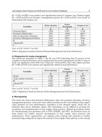
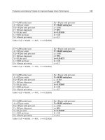
different circumstances are obtained, as shown in Table 2.

T
p
=1
−
<<
+
−
2
21 1
ii
w
ii
TT
T
TT
,
<
<01
i
T
>
+
2
21
i
w
i

T
T
T
, > 1
i
T
T
p
=2
−− − − + −− + − +
<<
−− −−
22
22
(3 9 2 1) (3 9 2 1)
2( 1) 2( 1)
iiii iiii
w
ii ii
T T TT T T TT
T
TT TT

<<0.5 1.618
i
T
−− − − +
>
−−
2

2
(3 9 2 1)
2( 1)
iiii
w
ii
TTTT
T
TT
> 1.618
i
T
T
a
=1,2
T
p
=3
−− +− − − ++
<<
+−−+
22 34
32
(4 2 3 8 4 16 1 16 )
2
21 2( 2 1)
ii i i i i i
i
w
iiii

TTT T T T T
T
T
TTTT

<<0 2.155
i
T

>
+
2
21
i
w
i
T
T
T
> 2.155
i
T
Table 2. Stability conditions of the APIOBPCS system
According to control engineering, a system’s stability condition only depends on the
parameters affecting feedback loop, as Table 2 shows. The stability boundary of DIS-
APIOBPCS is determined by T
p
, T
i
, and T

w
, whereas T
a
will not change the boundary. It is
interesting to note that the D–E line where T
i
= T
w
(Deziel and Eilon, 1967) always results in
a stable system and has other important desirable properties, as also reported in Disney and
Towill (2002).


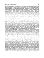
Fig. 3. The stability boundary when T
a
= 2 and T
p
= 2
0 1 2 3 4 5 6
0
1
2
3
4
5
6
7
Ti
Tw

Stable Region
Unstable
Region
Unstable Region
Ta=2,Tp=2 Stability condition
The Impact of Demand Information Sharing on the Supply Chain Stability

397
Thus it is important that system designers consider carefully about parameter settings and
avoid unstable regions. Given T
p
=2, the stable region of DIS-APIOBPCS is shown in Figure 3,
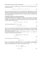
which also highlights six possible designs to be used as test cases of the stable criteria to a unit
step input. For sampled values of T
w
and T
i
, the exact step responses of the DIS-APIOBPCS
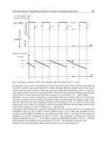
supply chain are simulated (Fig. 4) for stable; critically stable; and unstable designs.

0 5 10 15 20 25 30 35 40
-3000
-2000
-1000
0
1000
2000
3000
4000

Times (week s)
ORATE

0 10 20 30 40 50 60
0
0.2
0.4
0.6
0.8
1
1.2
1.4
1.6
Times (week s)
ORATE

(a) T
n
=4 T
w
=0 (point ○) (b) T
i
=4 T
w
=3 (point *)

0 5 10 15 20 25 30
-4
-3
-2

-1
0
1
2
3
4
5
6
Times(weeks)
ORATE

0 10 20 30 40 50 60 70 80 90 100
-3000
-2000
-1000
0
1000
2000
3000
4000
Times (week s)
ORATE

(c) T
i
=4 T
w
=0.8554 (point ●) (d) T
i
=1 T

w
=5 (point ×)
0 10 20 30 40 50 60 70 80 90 100
-2
-1
0
1
2
3
4
5
Times (week s)
ORATE

0 5 10 15 20 25 30 35 40 45 50
-3
-2
-1
0
1
2
3
4
x 10
4
Times (week s)
ORATE

(e) T
i

=1 T
w
=2 (point ▲) (f) T
i
=1 T
w
=0.2 (point △)
Fig. 4. Sampled dynamic responses of DIS-APIOBPCS
Supply Chain Management

398
These above plots conform the theory by clearly identifying the stable region for DIS-
APIOBPCS. The stable region provides supply chain operation a selected range for
parameter tuning. In other words, the size of the region reflects the anti-disturbance
capability of a supply chain system. As long as T
i
and T
w
are located in the stability region,
the supply chain could ultimately achieve stability regardless the form of the demand
information. While the parameters are located outside the stability region however, rather
than returning to equilibrium eventually, the system will appear oscillation. In real supply
chain systems, this kind of oscillation over production and inventory capacity will
inevitably lead system to collapse.
5. Dynamic response of DIS-APIOBPCS
Note that having selected stable design parameters, T
a
, T
i
, T

w
and T
p
significantly affect the
DIS supply chain response to any particular demand pattern. This section concentrates on
the fluctuations of ORATE, AINV and WIP dynamic response. There are various
performance measures under different forms of demand information. For demand signals in
forms of step and impulse, it is appropriate to use peak value, adjusted time and steady-
state error as measures of supply chain dynamic performance. For Gaussian process
demand, noise bandwidth will be a better choice. For other forms of demand information,
such as cyclical, dramatic and the combinations of the above, which measures should be
used still needs further investigation.
5.1 Dynamic response of DIS-APIOBPCS under step input
Within supply chain context, the step input to a production/inventory system may be
thought of as a genuine change in the mean demand rates (for example, as a result of
promotion or price reductions). A system’s step response usually provides rich insights
when seeking a qualitative understanding of the tradeoffs involved in the ‘‘tuning’’ of an
ordering policy (Bonney et al., 1994; John et al., 1994; Disney et al., 1997). Such responses
provide rich pictures of system behavior. A unit step input is a particularly powerful test
signal that control engineers to determine many properties of the system under study. For
example, the step is simply the integral of the impulse function, thus understanding the step
response automatically allows insight to be gained on the impulse response. This is very
useful as all discrete time signals may be decomposed into a series of weighted and delayed
impulses.
By simulation, a thorough understanding of the fundamental dynamic properties can be
clarified, which characterize the geometry of the step response with the following
descriptors.
Peak value: The maximum response to the unit step demand which reflects response
smoothness;
Adjusted time: transient time from the introduction of the step input to final value (±5

percent error) which reflect the rapidness of the supply chain response;
Steady-state error: I/O difference after system returns to the equilibrium state, which
reflects the accuracy of the supply chain response.
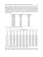
5.1.1 The impact of T
p
on DIS-APIOBPCS step response
As in real supply chain management environment, T
p
is a parameter which is hardly to
change frequently and artificially. No matter how T
p
is set, the steady-state error of ORATE,
The Impact of Demand Information Sharing on the Supply Chain Stability

399
AINV and WIP keeps zero. As shown in Figure 5, the smaller T
p
value, the smaller peak
value and shorter adjusted time. That is to say, when facing an expanding market demand,
supply chain members could try to shorten the production lead-time in order to lower
required capacity and accelerate response to market changes.

0 10 20 30 40 50 60
0
0.2
0.4
0.6
0.8
1
1.2

1.4
1.6
1.8
Time(weeks)
ORATE
Ta= 2 Ti= 3 Tw= 2


CONS
Tp= 1
Tp= 2
Tp= 3
0 10 20 30 40 50 60
-6
-5
-4
-3
-2
-1
0
1
Time(weeks)
AINV
Ta= 2 Ti= 3 Tw= 2


Tp= 1
Tp= 2
Tp= 3
CONS

DINV


(a) ORATE (b) AINV

0 10 20 30 40 50 60
0
0.5
1
1.5
2
2.5
3
3.5
4
4.5
5
Time(weeks)
WIP
Ta= 2 Ti=3 Tw= 2


CONS
Tp= 1
Tp= 2
Tp= 3
Tp= 1 DW IP
Tp= 2 DW IP
Tp= 3 DW IP

(c) WIP

Fig. 5. The impact of T
p
on DIS-APIOBPCS step response
5.1.2 The impact of T
w
on DIS-APIOBPCS step response
Fig.6 depicts the responses of DIS-APIOBPCS under different T
w
settings. It is shown that
given other parameters as constant, with T
w
increasing, the adjusted time of ORATE, AINV
and WIP responses and the peak value of ORATE response will first decline and then rise,
and the peak value of AINV and WIP responses will rise, while all the steady-state error will
remain zero. This means if the supply chain has a low production or stock capacity, when
the market demand is expanded, less proportion of WIP should be considered in order
quantity determination, to promote the performance and dynamic response of the supply
chain.
Supply Chain Management

400


1
1.2
1.4
1.6

1.8
2
2.2
2.4
2.6
0.9
1.2
1.4
1.6
2
4
6
8
10
Tw
Peak
0
5
10
15
20
25
30
35
40
Adjusted time
Peak
Adjusted time
3
3.5

4
4.5
5
5.5
1
1.3
1.5
1.8
3
5
7
9
Tw
Peak
0
10
20
30
40
50
60
Adjusted time
Peak
Adjusted time


(a) ORATE (b) AINV

2
2.5

3
3.5
4
4.5
5
1
1.2
1.3
1.4
1.5
1.6
1.8
2
3
4
5
6
7
8
9
Tw
Peak
0
5
10
15
20
25
30
35

40
45
Adjusted time
Peak
Adjusted time


(c) WIP

Fig. 6. The impact of T
w
on DIS-APIOBPCS step response
5.1.3 The impact of T
i
on DIS-APIOBPCS step response
Responses of DIS-APIOBPCS under different T
i
settings are shown in Fig.7. With other
parameters given, it can be found that the peak value of ORATE, AINV and WIP responses
will decline when T
i
increase, but the adjusted time follows a U-shaped process, and the
steady-state error keeps zero. This phenomenon indicates that when the market demand
expands, supply chain members must strike a balance between production, inventory
capacity and replenishment capabilities, and make a reasonable decision on inventory
adjustment parameter so as to maximize supply chain performance and to maintain long-
term and stable capability.
The Impact of Demand Information Sharing on the Supply Chain Stability

401

1
1.5
2
2.5
3
3.5
4
4.5
5
1
1.
2
1.
3
1.
4
1.
5
1.
6
1.
8
2
3
4
5
6
7

8
Ti
Peak
0
10
20
30
40
50
60
Adjusted time
Peak
Adjusted time
1
2
3
4
5
6
7
11.21.51.8234567
Ti
Peak
0
10
20
30
40
50
60

70
Adjusted time
Peak
Adjusted time


(a) ORATE (b) AINV

0
1
2
3
4
5
6
7
8
9
1
1.2
1.3
1.4
1.5
1.6
1.8
2
3
4
5
6

7
8
Ti
Peak
0
10
20
30
40
50
60
70
Adjusted time
Peak
Adjusted time


(c) WIP

Fig. 7. The impact of T
i
on DIS-APIOBPCS step response
5.1.4 The impact of T
a
on DIS-APIOBPCS step response
As shown in Fig.8, increasing T
a
is followed by declining peak value of ORATE and WIP
response and rising adjusted time, but the AINV peak value will first decline then rise. From
the analysis above, it is clear that T

a
should be reduced for the purpose of enhancing the
rapidness of the supply chain. But if the manager aims at production and inventory
smoothness, T
a
settings around 3.5 will be a reasonable choice.
From Section 5.1, it can be concluded that as long as the system parameters are located in
the stable region, the steady-state error of dynamic response will keep zero, which means
the requirement of response accuracy can always be met, whereas the smoothness and

Supply Chain Management

402
1.2
1.3
1.4
1.5
1.6
1.7
1.8
1
1.5
2
2.5
3
3.5
4
4.5
5
6

7
8
9
Ta
Peak
0
5
10
15
20
25
30
35
40
45
Adjusted time
Peak
Adjusted time
3.6
3.7
3.8
3.9
4.0
4.1
4.2
1 2 3 4 5 6 7 8 9 10 11 12 13
Ta
Peak
0
10

20
30
40
50
60
70
Adjusted time
Peak
Adjusted time

(a) ORATE (b) AINV
2.4
2.6
2.8
3
3.2
3.4
1
1.5
2
2.5
3
3.5
4
4.5
5
6
7
8
9

Ta
Peak
0
5
10
15
20
25
30
35
40
45
50
Adjusted time
Peak
Adjusted time

(c) WIP
Fig. 8. The impact of T
a
on DIS-APIOBPCS step response
rapidness of dynamic response sometimes have the contradictory requirements on system
parameter settings. For instance, the dynamic response of ORATE, AINV and WIP will be all
smoother and more rapid by decreasing T
p
, however, smoothness needs T
i
to stay low while
rapidness prefers a higher T
i

value. The supply chain members should adjust the system
parameters integratively for all the objectives of dynamic response so as to improve the
overall supply chain performance.
5.2 Dynamic response of DIS-APIOBPCS under impulse input
Demand in form of impulse can be seen as a sudden demand in the market. The sudden
demand appears frequently because there are a large number of uncertain factors in the
market competition environment. Sudden demand will have a serious impact on supply
chains, thus enterprises need to restore stability from this sudden change as soon as
possible, thereby reducing the volatility of the various negative effects.
5.2.1 The impact of T
p
on DIS-APIOBPCS impulse response
From Fig. 9, it can be seen that no matter how T
p
is set, the steady-state error of ORATE,
AINV and WIP keep zero. The smaller T
p
value, the smaller peak value and shorter adjusted
The Impact of Demand Information Sharing on the Supply Chain Stability

403
time. That is to say, when facing a sudden market demand, supply chain members could try
to shorten the production lead-time in order to restore supply chain stability.



0 5 10 15 20 25 30
-0.2
0
0.2

0.4
0.6
0.8
1
1.2
1.4
Times(weeks)
ORATE
Ta= 2 Ti=3 Tw= 2


Tp= 1
Tp= 2
Tp= 3
CONS
0 10 20 30 40 50 60
-1.5
-1
-0.5
0
0.5
1
Time(weeks)
AINV
Ta= 2 Ti=3 Tw= 2


Tp= 1
Tp= 2
Tp= 3

CONS


(a) ORATE (b) AINV

0 5 10 15 20 25 30 35 40
-0.2
0
0.2
0.4
0.6
0.8
1
1.2
1.4
1.6
1.8
Time(weeks)
WIP
Ta= 2 Ti=3 Tw= 2


Tp= 1
Tp= 2
Tp= 3
CONS


(c) WIP

Fig. 9. The impact of T
p
on DIS-APIOBPCS impulse response
5.2.2 The impact of T
w
on DIS-APIOBPCS impulse response
Fig.10 depicts that with other parameters given and the increase of T
w
, the adjusted time of
ORATE and WIP response will first decline and then rise, the adjusted time of AINV
response will decline when T
w
<6 and then rise. The peak value of ORATE declines; the peak
value of WIP will first decline then rise and eventually declines. But with the increase of T
w
,
the peak value of AINV response will rise.
Supply Chain Management

404

ORATE
0.6
0.7
0.8
0.9
1
1.1
1.2
1.3

1.4
1.5
1
1.2
1.5
1.8
2
3
4
5
6
7
8
9
10
Tw
Peak value
0
5
10
15
20
25
30
35
Adjusting time
Peak value
Adju s ting time
AINV
1

1.1
1.2
1.3
1.4
1.5
1.6
1.7
11.21.51.82345678910
Tw
Peak value
0
5
10
15
20
25
30
35
40
45
Adjusting tim e
Peak value
Adjusting time


(a) ORATE (b) AINV

WIP
1.2
1.25

1.3
1.35
1.4
1.45
1.5
11.21.51.62345678910
Tw
Peak value
0
5
10
15
20
25
30
Adjusting time
Peak value
Adjusting time


(c) WIP

Fig. 10. The impact of T
w
on DIS-APIOBPCS impulse response
5.2.3 The impact of T
i
on DIS-APIOBPCS impulse response
Impulse responses of DIS-APIOBPCS under different T
i

are shown in Fig.11. With other
parameters given, it can be found that the peak value of ORATE, AINV and WIP response
will decline when T
i
increases. The adjusted time of AINV response follows a process that
first decline and then rise; the adjusted time of ORATE and WIP response will decline. The
steady-state error keeps zero. This phenomenon indicates that when the market demand
bursts, supply chain members must strike a balance between production, inventory capacity
and recovery capabilities, and make a reasonable decision on inventory adjustment
parameter so as to maximize supply chain performance and maintain long-term and stable
operation.
The Impact of Demand Information Sharing on the Supply Chain Stability

405

ORATE
0
0.5
1
1.5
2
2.5
1
1.2
1.5
1.8
2
3
4
5

6
7
8
9
10
Ti
Peak value
0
10
20
30
40
50
60
Adjusting time
Peak value
Adjusting time
AINV
0.6
1.1
1.6
2.1
2.6
3.1
3.6
1 1.2 1.5 1.8 2 3 4 5 6 7 8 9 10
Ti
Peak value
0
5

10
15
20
25
30
35
40
45
50
Adjusting time
Peak value
Adjusting time


(a) ORATE (b) AINV

WIP
0
0.5
1
1.5
2
2.5
3
3.5
4
4.5
1.2 1.5 1.8 2 3 4 5 6 7 8 9 10
Ti
Peak value

0
5
10
15
20
25
30
Adjusting time
Peak value
Adjusting time


(c) WIP

Fig. 11. The impact of T
i
on DIS-APIOBPCS impulse response
5.2.4 The impact of T
a
on DIS-APIOBPCS impulse response
As shown in Fig.12, increasing T
a
is followed by declining peak value of ORATE, AINV and
WIP response and rising adjusted time. From the analysis above, it is clear that T
a
should be
reduced for the purpose of enhancing the rapidness of supply chain. But if the manager
aims at production and inventory smoothness, T
a
settings should be higher.

5.3 Dynamic response of the DIS-APIOBPCS under stochastic demand input
Noise bandwidth (W
n
) is commonly used in communication engineering system to measure
the inherent attributes of the system. It is defined as the area under the squared frequency
response of the system, expressed as Eq.(8).
Supply Chain Management

406

ORATE
0
0.2
0.4
0.6
0.8
1
1.2
1.4
1.6
1
1.5
2
2.5
3
3.5
4
4.5
5
6

7
8
9
Ta
Peak value
0
2
4
6
8
10
12
14
Adjusting time
Peak value
Adju s ting time
AINV
0.6
0.7
0.8
0.9
1
1.1
1.2
1.3
1.4
1.5
1.6
1 1.5 2 2.5 3 3.5 4 4.5 5 6 7 8 9
Ta

Peak value
0
5
10
15
20
25
30
35
40
Adjusting time
Peak value
Adjusting time


(a) ORATE (b) AINV

WIP
0
0.2
0.4
0.6
0.8
1
1.2
1.4
1.6
1.8
2
11.522.533.544.55 6 7 8 9

Ta
Peak value
0
5
10
15
20
25
Adjusting time
Peak value
Adjusting time


(c)WIP

Fig. 12. The impact of T
a
on DIS-APIOBPCS impulse response

π
=
∫
2
0
nf
WORATEdw (8)
Noise bandwidth is a performance measure that is proportional to the variance of the
ORATE response when the demand information consists of pure white noise (constant
power density at all frequencies), (Garnell and East, 1977 and Towill, 1999). Pure white noise
maybe interpreted as an independently and identically distributed (i.i.d.) normal

distribution. Thus, the noise bandwidth may be reasonably considered a surrogate metric
for production adaptation costs. These costs may include such factors as hiring/firing,
production on-costs, over-time, increased raw material stock holdings, obsolescence, lost
capacity etc. So when demand is i.i.d. form, the noise bandwidth can directly measure
fluctuations in production.
The Impact of Demand Information Sharing on the Supply Chain Stability

407
The relationship between W
n
and system parameters T
a
, T
i
and T
w
are shown in Fig.13.
2
4
6
8
2
4
6
8
0
10
20
30
40

Ti
Tw

Wn
WIP
ORATE
AINV

(a)
2
4
6
8 2
4
6
8
0
2
4
6
8
10
12
14

Ta
Ti

Wn

ORATE
AINV
WIP

(b)
Fig. 13. The impact of system parameters on dynamic response under stochastic input
The fluctuations of ORATE, AINV, and WIP response caused by demand fluctuations could
be reduced by tuning system parameters. From Fig.13, it can be concluded that the ORATE
and WIP fluctuation can be weakened by increasing T
a
and decreasing T
w
. The inventory
fluctuation can be weakened by increasing T
i
and reducing T
w
. Moreover, T
a
should be
Supply Chain Management

408
increased when T
i
is small, otherwise T
a
should be reduced. This shows that for members of
the supply chains, system fluctuation can be reduced by adjusting the system parameters in
feed-forward and feedback loops. However, when the inventory adjustment parameter T

i
is
a larger value, reducing inventory fluctuations has the opposite requirements on T
a
.
5.4 Dynamic response of the DIS-APIOBPCS under different order intervals
In Sections 5.1-5.3, this paper analyzes how the system parameters impact the system
dynamic responses to customer demand in forms of step, impulse, Gaussian Process in DIS-
APIOBPCS system. In this part, dynamic response to variant order intervals is studied. In
order to filter out the disturbance of random factors in simulation, demand information in
form of impulse will be appropriate. According to the step response of peak value and
adjusted time in DIS-APIOBPCS system, if T
w
takes 2, 3 or 4, the unit impulse response will
be more desirable, given T
a
=2, T
p
=2, T
i
=3 as shown in Fig.14. When T
w
=2, the unit impulse
response has a peak value of 1, but in other situations, the response will either has a higher
or lower peak value.




0 5 10 15 20 25 30 35 40

-1
-0.5
0
0.5
1
1.5
Time(weeks )
ORATE
Ta=2 Tp=2 Ti=3


Tw= 1
Tw= 2
Tw= 5
Tw= 8




Fig. 14. The impact of T
w
on DIS-APIOBPCS impulse response
From the simulation experiments under different order intervals from 1 to 10 week, the
maximum and minimum value of the response can be seen in Fig.15. When the order
interval is 1 week, the ORATE response has a minimum oscillation amplitude and the one of
WIP response is 0. The oscillation amplitude of AINV response will be minimal when the
order interval is 2 week as shown in Fig.16.
The Impact of Demand Information Sharing on the Supply Chain Stability

409

(a) ORATE (b) AINV



(c) WIP

Fig. 15. The maximum and minimum value of response under different order intervals
When the order interval of the supply chain is fixed, the system parameter setting will also
influence the dynamic response. With other parameters given, the optimal order interval of
ORATE response is still 1 week whether T
p
is increasing. However, the optimal order
interval of AINV and WIP response will increase with T
p
, and the increase of T
i
, T
w
and T
a

have no influence on the optimal order intervals. So it can be concluded that the optimal
order intervals will only be decided by the production lead-time no matter how much other
parameters are set. Because the page limits, this paper only gives the situation when T

p
=2
and T
p
=4, as shown in Figs.17 and 18.
Supply Chain Management

410

0 10 20 30 40 50 60 70 80
-0.2
0
0.2
0.4
0.6
0.8
1
1.2
Time(weeks)
ORATE
Ta=2 Tp= 2 Ti= 3 Tw= 2


ORATE
CONS

(a) ORATE
0 10 20 30 40 50 60 70 80 90 100
-1.5
-1

-0.5
0
0.5
1
Time(weeks)
AINV
Ta= 2 Tp=2 Ti =3 Tw=2


AINV
CONS


(b) AINV

0 10 20 30 40 50 60
-0.2
0
0.2
0.4
0.6
0.8
1
1.2
1.4
1.6
Time(weeks )
WIP
Ta=2 Tp=2 Ti=3 Tw=2

WIP
CONS

(c) WIP
Fig. 16. The dynamic response under optimal order interval
The Impact of Demand Information Sharing on the Supply Chain Stability

411



(1) ORATE

(2) AINV

(3) WIP

Fig. 17. The impact of order intervals on dynamic response when T
p
=2
Supply Chain Management

412



(1) ORATE

(2) AINV

(3) WIP

Fig. 18. The impact of order intervals on dynamic response when T
p
=4
The Impact of Demand Information Sharing on the Supply Chain Stability

413
6. Conclusions
Based on APIOBPCS model, this paper analyzes a demand information-sharing two-echelon
supply chain system model (DIS-APIOBPCS). The management significance of four key
parameters is analyzed and the stability condition under different lead-times is figured out.
The stability boundary is verified by simulation. Any parameters’ value beyond the stability
region will lead to instability of supply chain, thus it could be avoided via tuning
parameters of the feedback loops within the supply chain for a specific production lead-
time.
Then the system dynamic responses to customer demand in forms of stepwise, impulsive,
stochastic distribution and variant order intervals are analyzed. Regarding the step and
impulsive demand information input, the smaller the production lead-time, the lower the
peak value and the shorter the adjusted time. This means companies can reduce capacity
requirements when the market demand expands (and vice versa) by decreasing production
lead-times. T
i
and T
w
not only provide a means of ensuring stability, but also drive capacity
requirements to satisfy a step increase in demand. Supply chain members must strike a
balance between production, inventory capacity and recovery capabilities, and make a
reasonable decision on inventory adjustment parameters so as to maximize supply chain

performance and maintain long-term and stable operation. Under normally distributed
input, the noise bandwidth can directly measure fluctuations in production. The
fluctuations of ORATE, AINV, and WIP response caused by demand fluctuations could be
reduced by tuning system parameters. The optimal order intervals will only be affected by
the production lead-time.
The DIS-APIOBPCS system model could be expanded to any two enterprises in multi-
echelon supply chain systems and those using other information sharing strategies.
Furthermore, research on stability condition and dynamic response under other demand
information forms is an important problem in supply chain management.
7. Acknowledgement
The work reported in this paper was supported by the National Natural Science Foundation
of China (No. 70572014; 70821061; 70872009).
8. References
Dejonckheere J., Disney S.M., Lambrecht M.R., Towill D.R. Measuring and avoiding the
Bullwhip Effect: a control theoretic approach. European Journal of Operations
Research, 2003,147 (3), 567–590.
Dejonckeere J., et al. The impact of information enrichment on the bullwhip effect in supply
chains: a control engineering perspective, Euro. J. Operational Res. 2004, 153(3):

727-750.
Disney S.M., Naim M.M., Towill D.R. Genetic algorithm optimization of a class of inventory
control systems. International Journal of Production Economics 2000, 68:259–78.
Disney S.M., Towill D.R. A discrete transfer function model to determine the dynamic
stability of a vendor managed inventory supply chain. International Journal of
Production Research, 2002, 40 (1), 179–204.
Supply Chain Management

414
Disney S.M., Towill D.R. On the Bullwhip and inventory variance produced by an ordering
policy. The International Journal of Management Science, 2003, 31(3): 157–167.

Disney S.M., Towill D.R., Van de Velde, W. Variance amplification and the golden ratio in
production inventory control systems. International Journal of Production
Research, 2004, 90 (3), 295–309.
Disney S M. Towill D.R. Eliminating drift in inventory and order based production control
systems. International Journal of Production Economics, 2005, 93–94: 331-344.
Disney S.M., Towill D.R., Warburton, R.D.H. On the equivalence of control theoretic,
differential, and difference equation approaches to modeling supply chains.
International Journal of Production Economics, 2006, 101 (1), 194–208.
Warburton R.D.H., Disney S.M. Order and inventory variance amplification: The
equivalence of discrete and continuous time analyses. International Journal of
Production Economics, 2007, 110(1-2): 128-137.
Fernanda Strozzi, Carlo Noè, José-Manuel Zaldívar. The Control of Local Stability and the
Bullwhip Effect in a Supply Chain. International Journal of Production Economics,
2007, 12:1-11.
Forrester J.W. Industrial Dynamics. MIT Press, Cambridge, MA. 1961
Sarimveis H., et al. Dynamic modeling and control of supply chain systems: A review.
Computers and operations research, 2008, 35(11): 3530-3561.
Khalid Saee. Trend forecasting for stability in supply chains. Journal of Business Research,
Available online 16 January 2008.
Lalwani C.S., Disney S.M., Towill D.R. Controllable, observable and stable state space
representations of Order-up-to policy. International Journal of Production
Economics, 2006, 101:172-184
Nordin Saad, Visakan Kadirkamanathan. A DES Approach for the Contextual load
modeling of Supply Chain System for Instability Analysis. Simulation Modeling
Practice and Theory, 2006, 14:541-563
Riddalls C.E., Bennett S. The stability of supply chains. International Journal of Production
Research, 2002, 40 (2), 459–475.
Takashi Nagatani, Dirk Helbing. Stability Analysis and Stabilization Strategies for Linear
Supply Chains. Physica A, 2004:633-660.
Towill D.R. Dynamic analysis of an inventory and order based production control system.

International Journal of Production Research .1982;20:671–87.
Towill D.R. Industrial dynamics modeling of supply chains. International Journal of
Physical Distribution &Logistics Management, 1996,26(2):23~42.
Vassian H.J. Application of discrete variable servo theory to inventory control. Operations
Research, 1954. 3, 272–282.
Warburton R.D.H. An analytical investigation of the Bullwhip Effect. Production and
Operations Management , 2004a, 13 (1), 150–160.
Warburton R.D.H. An exact solution to the production inventory control system.
International Journal of Production Economics, 2004b, 92 (1), 81–96.
Warburton R.D.H., Disney S.M., Towill D.R., Hodgson J.P.E. Further insights into the
stability of supply chains. International Journal of Production Research, 2004, 42 (3),
639–648.
Yanfeng Ouyang. The effect of information sharing on supply chain stability and the
bullwhip effect. European Journal of Operational Research.2007, 182(3),1107-1121.
Part 3
Modeling and Analysis