Supply Chain Management Part 13 pdf

Quantifying the Demand Fulfillment Capability of a Manufacturing Organization

471
• The consumer’s behavior (demand uncertainty) impacts the planning horizon of the
market opportunity. In this way, demand uncertainty determines the level of customer
feedback provided by the business model, i.e. as the demand becomes more
unpredictable, no planning ahead of time can not take place and there is the need to
wait for customer info.
• The business model establishes the Organization’s approach to the identified market
opportunity, understood in terms of order winners/qualifiers. In this way, the business
model relies on the process environment, i.e. a make-to-stock (MTS) business model
that requires having always ready-to-sell finished goods, must be supported by a mass
production environment that produces high volumes of short-lead time products.
• The market opportunity is translated into a specific product. The capability of the
Organization to manufacture different varieties of products depends in great deal on
how much standardized the products’ BOM structures are (as they allow the use of
postponement and/or modularization approaches). In this way, product
standardization allows the achievement of the order winners/qualifiers, i.e. the order
winners/qualifiers delivery, cost, and quality are achievable when the product is of
simple assembly.
• The process required to produce a product have time components that are greatly
influenced by product’s features (operations complexity, i.e. level of standardization)
and process’ capabilities (operations uncertainties, i.e. production volumes). In this
way, the process environment is conditioned by the product standardization, i.e. a
product with high levels of standardization (and simple to produce) allows high levels
of production volumes.
It must be noted that there are four recurrent elements present in these alignment
conditions: demand uncertainty, business model, product standardization, and process
environment flexibility. In the next section we use these four elements to derive an
analytical expression of the impact the strategic - operational levels alignment has on the
performance of the manufacturing organization. Section 3 illustrates the usefulness of the

analytical expression via the development of a simulation model, section 4 shows the
sensitivity analysis performed over the proposed simulation model, and section 5 closes
with the conclusions and future research.
2. Analytical expression of the demand fulfillment capability
According to [16] and [17], metrics used to measure the performance of the SC can be
classified as strategic, tactical, and operational, where the performance of a SC partner can
be expressed in terms such as customer satisfaction, product quality, speed in completing
manufacturing orders, productivity, diversity of product line, flexibility in manufacturing
new products, etc [18]. In this paper we use demand fulfillment - understood as the
achievement of the demanded volume - as it relates to the four recurrent elements present in
the alignment conditions of the previous section:
• Demand uncertainty (U); according to [19], when demand uncertainty is low, a make-
to-stock (MTS) business model is recommended. When demand uncertainty is high, a
make-to-order (MTO) business model is recommended.
• Business model (BM); according to [20], in a MTS business model production planning is
made based on a forecast (rather than actual orders), allowing to produce ahead of time,
Supply Chain Management

472
keep a stock, and ship upon receipt of orders. According to [21], when using this business
model, an inventory-oriented level strategy should be used, where a steady production is
maintained and finished goods inventory is used to absorb ongoing differences between
output and sales. In the case of the case of the MTO business model, according to [20],
production planning is made on actual orders (rather than on forecast), allowing to
eliminate finished goods inventories. When using this business model, a capacity-oriented
chase strategy should be used [21], where the expected demand is tracked and the
corresponding capacity is computed, raising it or lowering it accordingly.
• Process environment flexibility (F); according to [19], when following a level strategy, a
rigid continuous production line should be used. When following a chase strategy, a
flexible job shop should be used.

• Product standardization (S); according to [22], a continuous production line uses
special-purpose equipment - grouped around the product - to profitably manufacture
high-volumes of standardized products. In the case of the of the job shop, it uses
general-purpose equipment - grouped around the process – to profitably manufacture
low-volumes of customized products.
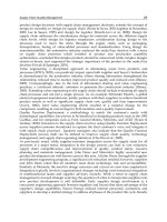
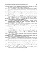
As we can see in Figure 1, there is trade-off between the inventory-oriented and capacity-
oriented strategies (or demand fulfillment strategies): the contribution increase/decrease of
one implies the contribution decrease/increase of the other. This can be express in an
analytical way:
• When uncertainty U is low (0), business model BM is MTS (0), standardization S is high
(1), and flexibility F is low (0), demand is fulfilled 100% from inventory, Equation (1):
Inventory contribution to demand fulfillment = D * (1-U) * (1-BM) * S * (1-F) (1)
• When uncertainty U is high (1), business model BM is MTO (1), standardization S is low
(0), and flexibility F is high (1), demand is fulfilled 100% from capacity, Equation (2):
Capacity contribution to demand fulfillment = D * U * BM *(1- S) * F (2)

Inventory-oriented
strategy
Capacity-oriented
strategy
BM = 0
U = 0
S = 1
F = 0
BM = 1
U = 1
S = 0
F = 1

Fig. 1. Demand fulfillment relationships

In this way, demand fulfillment would be sum of the contributions made by the inventory-
oriented and capacity-oriented strategies: for a totally aligned scenario (left or right sides of
Figure 1), demand will be fulfilled by a 100% inventory-oriented or 100% capacity-oriented
strategy; for a misaligned scenario, demand will be fulfilled by a combination of both
Quantifying the Demand Fulfillment Capability of a Manufacturing Organization

473
strategies. Table 3 presents all the different combinations of limit conditions (that is, the 0’s
or 1’s in Table 2), for a demand level of 100 units. As we can see, Equation (1) and (2)
represent accurately the trade-off between the demand fulfillment strategies. Note: when the
demand fulfillment equals to zero it means that even though some level of production takes
place, the achieved demand volume is really low - when compared to the demanded
volume - that it can be considered to be zero. For example, if demand equals to 100 units,
there is high uncertainty in the demand (U = 1), the business model used is MTO (BM = 1),
the product is totally standardized (S = 1), and it uses a functional job shop (F = 1). Here the
high uncertainty of the demand requires waiting for customer feedback (provided by the
MTO business model). However, the totally standardized product is characterized by using
simple manufacturing and/or assembly operations (that take a really short time). In this
case, the functional job shop used would affect the fulfillment of the 100 units, by presenting
two obstacles to the flow of the process: 1) the set up times proper of the universal
equipment used (very long compared to the production run), and 2) the moving time from
one operation to the next (as all the equipment is grouped based on their functionality). In
this way, the analytical expression of the alignment impact can not be taken as an estimator
of the final values of the fulfilled demand, but instead, as an indicator of the capability of the
manufacturing organization to achieve the demanded volume (or demand fulfillment
capability indicator): the closer this indicator is to the demand volume, the more feasible it
will be for the manufacturing organization to achieve the demanded volume.
Before proceeding to the next section, it must be noted that the customer service and the
demand fulfillment relationships (presented in the previous sections), are well-known facts -
by production managers and industrial engineers - that have been reported previously in

the literature. What we consider to be an original contribution of this paper is taking these
well-known facts of production engineering, and putting them in the form of the demand
fulfillment capability indicator, an analytical expression that relates the degree of alignment
(between the structural and operational levels) with demand fulfillment. Two similar
demand fulfillment equations are presented in [23], but they only consider the uncertainty
and business model configuration attributes. In our proposal, we extend that work by
including the standardization and flexibility configuration attributes. Next section present
the practical applications (and therefore its usefulness) of the derived analytical expression.

0 0.25 0.5 0.75 1
Uncertainty
Low, std = 0%
of demand
Low-medium,
std = 7.5% of
demand
Medium, std =
15% of demand
Medium-high,
std = 22.5% of
demand
High, std
= 30% of
demand
Business model MTS MTS-ATO ATO ATO-MTO MTO
Standardization
Customer’s
specs
Own catalog,
non-standard

options
Own catalog,
with standard
options
Standard with
options
Standard,
no options
Flexibility
Mass assembly
line
Repetitive U
line
Batch U line Batch cellular
Functional
job shop
Table 2. Numeric values of the recurrent elements
Supply Chain Management

474

Demand fulfillment strategy
100%
inventory-
-oriented
100%
Capacity-
-oriented

D 100 100 100 100 100 100 100 100 100 100 100 100 100 100 100 100

U 0 1 0 0 0 1 1 1 0 0 0 1 1 1 0 1
BM 0 0 1 0 0 1 0 0 1 1 0 1 1 0 1 1
S 0 0 0 1 0 0 1 0 1 0 1 1 0 1 1 1
F 0 0 0 0 1 0 0 1 0 1 1 0 1 1 1 1
Equation (1) result 0 0 0
100
0 0 0 0 0 0 0 0
0
0 0 0
Equation (2) result 0 0 0
0
0 0 0 0 0 0 0 0
100
0 0 0
Table 3. Results for different combinations of limit conditions
3. Practical application of the demand fulfillment capability indicator
Reference [24] presents the case of Company ABC, a furniture company experiencing
unforeseen problems due to the implementation of company-wide policies that put into
conflicts the alignment relationships (between the strategic and operational levels)
mentioned in section 1.1. The impact these policies have on Company ABC’s performance,
can be evaluated by using Equation (1) and (2) and the following values (from Table 2):
• U = 0.25, for a somewhat predictable market demand.
• BM = 0.5, for having products stocked in a ready-to-assemble condition.
• S = 0.25, for the offered own catalog – no standards options.
• F = 0.75, for the use of manufacturing cells.
In this way, for a demand level of 100 units, the demand fulfillment feasibility indicator
shows a total value of 9.37 (meaning that Company ABC has a really hard time trying to
achieve the demanded volume of 100 units):

Inventory contribution = 100 * (1-0.25) * (1-0.5) * 0.25 * (1-0.75) = 2.34

Capacity contribution = 100 * 0.25 * 0.5 *(1- 0.25) * 0.75…………… = 7.03
Total = 9.37
At this point, Company ABC needs to explore the possibility of making some adjustments to
their policies, by migrating from their current alignment conditions to new ones. This
migration process implies either increasing or decreasing some of the business model,
standardization, and/or flexibility values. Examples of such migration process can be found
in [14]. The question becomes then which values to increase/decrease and in what amount.
An alternative that Company ABC has to answer these questions is the development of a
simulation model that guides its search for more advantageous alignment conditions. Some
important business applications of simulation within SC scenarios are:
• A simulation model is generally accepted as a valuable aid for gaining insights into and
making decisions about the manufacturing system [25].
• A simulation model provides a mean to evaluate the impact of policy changes and to
answer ‘what if?’and ‘what’s best?’ questions [26].
• A simulation model is useful for performance prediction [27] and for representing time
varying behaviors [28].
• A simulation model is maybe the only approach for analyzing the complex and
comprehensive strategic level issues that need to consider the tactical and operational
levels [29].
Quantifying the Demand Fulfillment Capability of a Manufacturing Organization

475
For this reason, and in order to show the practical use of our research contribution,
Equations (1) and (2), in this paper we proceed in the following way:
• Develop of a simulation model of an automotive SC partner; following a similar
approach to the one presented by [30], where a discrete event simulation model (of a
SC) is implemented and an application example is proposed for a better understanding
of the simulation model potential. The reason for choosing the case of an automotive SC
partner obeys to the following reason: [31] presents a SC modeling methodology and
uses the automotive SC in order to exemplify it. It must be noted that point 3 of the

modeling methodology presented in [31] assumes that the demand fulfillment
capability, of the partners within the automotive SC, depends only on the business
model used. This is where we consider our research contribution can complement the
modeling methodology presented in [31], by adding the uncertainty, standardization,
and flexibility elements (Equations 1 and 2).
• Use of system dynamics (SD) as the simulation paradigm; following a similar approach
to the one presented by [32], where a SD is employed to analyze the behavior and
operation of a hybrid push/pull CONWIP-controlled lamp manufacturing SC. SD is
one of the four simulation types mentioned by [33], and it is a system thinking
approach that is not data driven, and that focuses on how the structure of a system and
the taken policies affect its behavior [34]. According to [32], SD can be applied from
macro perspective modeling (SC system) to micro perspective modeling (production
floor system), and when applied to SC systems, it allows the analysis and decision on
an aggregate level (which is more appropriate for supporting management decision-
making, than conventional quantitative simulation).
Within this context, we use Equations (1) and (2) to develop an SD simulation model and
use the situation of the automotive SC partner as an application example. In the case the
simulation model is used as a decision making tool, then a Design of Experiment (DOE) or
an Analysis of Variance (ANOVA) needs to be perform on the statistical analysis of the
output, as the result of the decision making process depends on how experiments are
planned and how experiments results are analyzed.
3.1 Simulation model of an automotive SC partner
Based on Equations (1) and (2), an SD simulation model was built using the simulation
software [35]. The SD simulation model was verified and validated following a similar
approach to the one in [36]: it was presented to experienced professionals in the area of
simulation model building, and the simulation model output was examined for
reasonableness under a variety of settings of input parameters. The SD simulation model
developed for a partner of the automotive SC is presented in Figure 2. This model complies
with the analytical model presented by [31]:
1. The SC has several independent partners.

2. There is no global coordinator to make decisions at all levels, decisions are made locally
and decentralized.
3. The partners have only two kinds of inputs and outputs, material and information
flows. Material and information flows are described using inventory level and order
backlog equations.
4. Each partner operates as a pull system (driven by orders between the partners involved
in the SC) that processes or satisfies orders only when it has a backlog or orders to be
processed.
Supply Chain Management

476
5. Each partner can handle one product family (i.e. wipers) or one a single product (i.e. a
specific type of wiper). For SC of the automotive industry, modeling partners that are
able only to handle one product represents a sufficient and realistic requirement.


Fig. 2. SD simulation model of an automotive supply chain partner, as proposed by [31]
The performance criteria considered is demand fulfillment (in the form of the accumulated
total backlog at the end of planning period T). The most important assumptions made in the
simulation model are the following:
• Total backlog
i
is the difference between Demand
i
and Supply
i
, during period i of the
planning period T.
• Demand
i

varies according to a normal distribution, with a mean of 100 units and a
standard deviation of Uncertainty. The normal distribution is used to represent a
symmetrically variation above and below a mean value [37].
• Uncertainty

ranges from 0 units (low) to 30 units (high).
• Supply
i
is equal to supply
i
OUT.
• Supply
i
OUT is equal to Supply
i
IN after a delay of lead time
i
.
• Lead time
i
varies according to a uniform distribution and is given in weeks. The uniform
distribution is used to represent the ‘worst case’ result of variances in the lead time [37].
• Supply
i
IN is the sum of the contribution made by Inventory
i
and Capacity
i
. This is done
with the intention to reflect the different demand fulfillment strategies, i.e. level

strategy (inventory-oriented) for MTS environments and chase strategy (capacity-
oriented) for MTO environments.
• Business model ranges from 0 (MTS environment) to 1 (MTO environment).
• Standardization ranges from 0 (low) to high (1).
• Flexibility ranges from 0 (low) to high (1).
Quantifying the Demand Fulfillment Capability of a Manufacturing Organization

477
• Inventory
i
is equal to Equation (1):
Demand * (1- Uncertainty) * (1- Business model) * Standardization * (1- Flexibility)
• Capacity P
i
is equal to Equation (2):
Demand * Uncertainty * Business model * (1- Standardization) * Flexibility
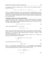
Figure 3 shows the analysis of a partner of the automotive supply chain. Stock elements were
used to represent the Backlog P
i
, due to its accumulating nature, while Conveyor elements were
used to represent the delay of lead time units for fulfilling the order, due to its transit time
feature.







= Supply OUT = 100 + Normal (0, uncertainty)

= Demand - Supply
= Inventory + Capacity Transit time = Lead time
= Demand*(Uncertainty/30)*Business model*(1-Standardization)*Flexibility
= Demand* (1- Uncertainty/30 )*(1-Business model)*Standardization*(1-Flexibility)

Fig. 3. Explanation of the elements of the SD simulation model
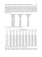
4. Sensitivity analysis
In order to study the effect of varying the level of demand uncertainty and lead time
variation, 1875 different scenarios were tested:
• Uncertainty levels of 0, 7.5, 15, 22.5, and 30. As it was stated previously, these values
represent the standard deviation (given in units) of the normal distribution used to
represent the demand variation.
• Business model, Standardization, and Flexibility levels of 0, 0.25, 0.5, 0.75, and 1.
• Lead time levels of Uniform (1, 1), Uniform (1, 3), and Uniform (1, 5). In a uniform
distribution, values spread uniformly between a minimum and a maximum value. In this
way, Uniform (1,1) represent a low lead time variation (no variation), Uniform (1,3)
represent medium lead time variation (values spread between 1 and 3 weeks), and
Uniform (1,5) represent a high lead time variation (values spread between 1 and 5 weeks).
For a planning period T = 100 and thirty replications per scenario, confidence intervals of
95% level were constructed and reported in Tables 4, 5, and 6, which summarize the
behavior of the total backlog values as standardization, flexibility, and business model
increases from 0 to 1, uncertainty increases from 0 to 30, and lead time increases from low -
Uniform (1, 1) - to high - Uniform (1, 5).
Supply Chain Management

478
03 = u 5.22 = u 51 = u
5
.
7

=
u
0
=
u
s
s
s s s
bm f 0 0.25 0.5 0.75 1 0 0.25 0.5 0.75 1 0 0.25 0.5 0.75 1 0 0.25 0.5 0.75 1 0 0.25 0.5 0.75 1
0
10000 7525 5050 2575 100 9949.47 8142 6286.03 4429.3 2572.43 9949.5 8760.77 7523.13 6285.57 5047.6 9948.47 9379.5 8760.03 8140.87 7521.43 9948.73 9948.73 9948.73 9948.73 9948.73
0.25
10000 8218 6337 4456 2575 9949.47 8605.9 7214 5821.7 4429.3 9949.5 9070.63 8141.53 7213.3 6285.57 9948.47 9533.97 9069.43 8605.67 8140.87 9948.73 9948.73 9948.73 9948.73 9948.73
0.5
10000 8812 7525 6337 5050 9949.47 9070.7 8142 7214 6286.03 9949.5 9377.79 8760.77 8141.53 7523.13 9948.47 9688.57 9379.5 9069.43 8760.03 9948.73 9948.73 9948.73 9948.73 9948.73
0.75
10000 9406 8812 8218 7525 9949.47 9537.23 9070.7 8605.9 8142 9949.5 9688.23 9379.77 9070.63 8760.77 9948.47 9845.07 9688.57 9533.97 9379.5 9948.73 9948.73 9948.73 9948.73 9948.73
0
1
10000 10000 10000 10000 10000 9949.47 9949.47 9949.47 9949.47 9949.47 9949.5 9949.5 9949.5 9949.5 9949.5 9948.47 9948.47 9948.47 9948.47 9948.47 9948.73 9948.73 9948.73 9948.73 9948.73
0
10000 8218 6337 4456 2575 9949.47 8605.9 7214 5821.7 4429.3 9949.5 9070.63 8141.53 7213.3 6285.57 9948.47 9533.97 9069.43 8605.67 8140.87 9948.73 9948.73 9948.73 9948.73 9948.73
0.25
10000 8614 7228 5842 4456 9850.47 8838.1 7833.47 6827.63 5821.7 9688.23 9070.63 8451.13 7831.87 7213.3 9533.97 9302.47 9069.43 8836.77 8605.67 9378.77 9533.43 9688.37 9844 9948.73
0.5
10000 9109 8218 7228 6337 9681.83 9070.7 8452.37 7833.47 7214 9379.77 9070.63 8760.77 8451.13 8141.53 9069.43 9069.43 9069.43 9069.43 9069.43 8760.03 9069.93 9378.77 9688.37 9948.73
0.75
10000 9604 9109 8614 8218 9537.23 9301.93 9070.7 8838.1 8605.9 9070.63 9070.63 9070.63 9070.63 9070.63 8605.67 8836.77 9069.43 9302.47 9533.97 8140.53 8604.27 9069.93 9533.43 9948.73
0.25
1

10000 10000 10000 10000 10000 9379.4 9537.23 9681.83 9850.47 9949.47 8760.77 9070.63 9379.77 9688.23 9949.5 8140.87 8605.67 9069.43 9533.97
9948.47 7521.67 8140.53 8760.03 9378.77 9948.73
0
10000 8812 7525 6337 5050 9949.47 9070.7 8142 7214 6286.03 9949.5 9379.77 8760.77 8141.53 7523.13 9948.47 9688.57 9379.5 9069.43 8760.03
9948.73 9948.73 9948.73 9948.73 9948.73
0.25
10000 9109 8218 7228 6337 9681.83 9070.7 8452.37 7833.47 7214 9379.77 9070.63 8760.77 8451.13 8141.53 9069.43 9069.43 9069.43 9069.43 9069.43 8760.03 9069.93 9378.77 9688.37 9948.73
0.5
10000 9406 8812 8218 7525 9379.4 9070.7 8762.03 8452.37 8142 8760.77 8760.77 8760.77 8760.77 8760.77 8140.87 8450.33 8760.03 9069.43 9379.5 7521.67 8140.53 8760.03 9378.77 9948.73
0.75
10000 9703 9406 9109 8812 9070.7 9070.7 9070.7 9070.7 9070.7 8141.53 8451.13 8760.77 9070.63 9379.77 7212.03 7826.4 8450.33 9069.43 9688.57 6283.8 7210.97 8140.53 9069.93 9948.73
0.5
1
10000 10000 10000 10000 10000 8762.03 9070.7 9379.4 9681.83 9949.47 7523.13 8141.53 8760.77 9379.77 9949.5 6283.7 7212.03 8140.87 9069.43 9948.47 5044.73 6283.8 7521.67 8760.03 9948.73
0
10000 9406 8812 8218 7525 9949.47 9537.23 9070.7 8605.9 8142 9949.5 9688.23 9379.77 9070.63 8760.77 9948.47 9845.07 9688.57 9533.97 9379.
5 9948.73 9948.73 9948.73 9948.73 9948.73
0.25
10000 9604 9109 8614 8218 9537.23 9301.93 9070.7 8838.1 8605.9 9070.63 9070.63 9070.63 9070.63 9070.63 8605.67 8836.77 9069.43 9302.47 9533.97 8140.53 8604.27 9069.93 9533.43 9948.73
0.5
10000 9703 9406 9109 8812 9070.7 9070.7 9070.7 9070.7 9070.7 8141.53 8451.13 8760.77 9070.63 9379.77 7212.03 7832.3 8450.33 9069.43 9688.57 6283.8 7210.97 8140.53 9069.93 9948.73
0.75
10000 9901 9703 9604 9406 8605.9 8838.1 9070.7 9301.93 9537.23 7213.3 7831.87 8451.13 9070.63 9688.23 5280.03 6825.23 7832.3 8836.77 9845.07 4425.7 5818.9 7210.97 8604.27 9948.73
0.75
1
10000 10000 10000 10000 10000 8142 8605.9 9070.7 9537.23 9949.47 6285.57 7213.3 8141.53 9007.63 9949.5 4426.9 5820.03 7212.03 8605.67 99
48.47 2568.33 4425.7 6283.8 8140.53 9948.73
0
10000 10000 10000 10000 10000 9949.47 9949.47 9949.47 9949.47 9949.47 9949.5 9949.5 9949.5 9949.5 9949.5 9948.47 9948.47 9948.47 9948.47 9
948.47 9948.73 9948.73 9948.73 9948.73 9948.73

0.25
10000 10000 10000 10000 10000 9379.4 9537.23 9681.83 9850.47 9949.47 8760.77 9070.63 9379.77 9688.23 9949.5 8140.87 8605.67 9069.43 9533.97 9948.47 7521.67 8140.53 8760.03 9378.77 9948.73
0.5
10000 10000 10000 10000 10000 8762.03 9070.7 9379.4 9681.83 9949.47 7523.13 8141.53 8760.77 9379.77 9949.5 6283.7 7212.03 8410.87 9069.43 9948.47 5044.73 6283.8 7521.67 8760.03 9948.73
0.75
10000 10000 10000 10000 10000 8142 8605.9 9070.7 9537.23 9949.47 6285.57 7213.3 8141.53 9070.63 9949.5 4426.9 5820.03 7212.03 8605.67 9948.47 2568.83 4425.7 6283.8 8140.53 9948.73
1
1
10000 10000 10000 10000 10000 7523.83 8142 8762.03 9379.4 9949.47 5047.6 6283.57 7523.13 8760.77 9949.5 2568.77 4426.9 6283.7 8140.87 9948.47 91.73 2568.83 5044.73 7521.67 9948.73

Table 4. Simulation output, low lead time variation
Quantifying the Demand Fulfillment Capability of a Manufacturing Organization

479
03 = u 5.22 = u 51 = u
5
.
7
= u 0 =
u
s
s
s s s
bm f 0 0.25 0.5 0.75 1 0 0.25 0.5 0.75 1 0 0.25 0.5 0.75 1 0 0.25 0.5 0.75 1 0 0.25 0.5 0.75 1
0
10000 7560.83 5121.67 2682.5 243.33 9949.47 8167.73 6338.07 4507.9 2677.33 9949.5 8777.4 7557.1 6336.83 5116.27 9948.47 9387.17 8776.23 8165.57 7554.67 9948.73 9948.73 9948.73 9948.73 9948.7
3
0.25
10000 8243.8 6390.03 4536.27 2682.5 9949.47 8625.1 7253 5880.4 4507.9 9949.5 9083 8166.87 7251.63 6336.83 9948.47 9539.53 9081.37 8624.17 8165.57 9948.73 9948.73 9948.73 9948.73 9948.7
3

0.5
10000 8829.2 7560.83 6390.03 5121.67 9949.47 9083.23 8167.73 7253 6338.07 9949.5 9387.7 8777.4 8166.87 7557.1 9948.47 9691.93 9387.17 9081.37 8776.23 9948.73 9948.73 9948.73 9948.73 9948.7
3
0.75
10000 9414.6 8829.2 8243.8 7560.83 9949.47 9543.17 9083.23 8625.1 8167.73 9949.5 9691.87 9387.7 9083 8777.4 9948.47 9846.37 9691.93 9539.53 9387.17 9948.73 9948.73 9948.73 9948.73 9948.7
3
0
1
10000 10000 10000 10000 10000 9949.47 9949.47 9949.47 9949.47 9949.47 9949.5 9949.5 9949.5 9949.5 9949.5 9948.47 9948.47 9948.47 9948.47 9948.47 9948.73 9948.73 9948.73 9948.73 9948.7
3
0
10000 8243.8 6390.03 4536.27 2682.5 9949.47 8625.1 7253 5880.4 4507.9 9949.5 9083 8166.87 7251.63 6336.83 9948.47 9539.53 9081.37 8624.17 8165.57 9948.73 9948.73 9948.73 9948.73 9948.7
3
0.25
10000 8634.07 7268.13 5902.2 4536.27 9851.9 8853.97 7863.63 6871.97 5880.4 9691.87 9083 8472.1 7861.5 7251.63 9539.53 9311.3 9081.37 8852.13 8624.17 9386.43 9539.07 9691.8 9845.37 9948.7
3
0.5
10000 9121.9 8243.8 7268.13 6390.03 9685.57 9083.23 8473.6 7863.63 7253 9387.7 9083 8777.4 8472.1 8166.87 9081.37 9081.37 9081.37 9081.37 9081.37 8776.1 9081.67 9386.43 9691.8 9948.7
3
0.75
10000 9609.73 9121.9 8634.07 8243.8 9543.17 9311.17 9083.23 8853.97 8625.1 9083 9083 9083 9083 9083 8624.17 8852.13 9081.37 9311.3 9539.53 8164.93 8622.43 9081.67 9539.07 9948.7
3
0.25
1
10000 10000 10000 10000 10000 9387.47 9543.17 9685.57 9851.9 9949.47 8777.4 9083 9387.7 9691.87 9949.5 8165.57 8624.17 9081.37 9539.53 9948.47 7554.5 8164.93 8776.1 9386.43 9948.7
3
0
10000 8829.2 7560.83 6390.03 5121.67 9949.47 9083.23 8167.73 7253 6338.07 9949.5 9387.7 8777.4 8166.87 7557.1 9948.47 9691.93 9387.17 9081.37 8776.23 9948.73 9948.73 9948.73 9948.73 9948.7
3
0.25

10000 9121.9 8243.8 7268.13 6390.03 9685.57 9083.23 8473.6 7863.63 7253 9387.7 9083 8777.4 8472.1 8166.87 9081.37 9081.37 9081.37 9081.37 9081.37 8776.1 9081.67 9386.43 9691.8 9948.7
3
0.5
10000 9414.6 8829.2 8243.8 7560.83 9387.47 9083.23 8778.9 8473.6 8167.73 8777.4 8777.4 8777.4 8777.4 8777.4 8165.57 8470.87 8776.23 9081.37 9387.17 7554.5 8164.93 8776.1 9386.43 9948.7
3
0.75
10000 9707.3 9414.6 9121.9 8829.2 9083.23 9083.23 9083.23 9083.23 9083.23 8166.87 8472.1 8777.4 9083 9387.7 7249.67 7861.33 8470.87 9081.37 9691.93 6333.33 7247.9 8164.93 9081.67 9948.7
3
0.5
1
10000 10000 10000 10000 10000 8778.9 9083.23 9387.47 9685.57 9949.47 7557.1 8166.87 8777.4 9387.7 9949.5 6333.97 7249.67 8165.57 9081.37
9948.47 5110.97 6333.33 7554.5 8776.1 9948.7
3
0
10000 9414.6 8829.2 8243.8 7560.83 9949.47 9543.17 9083.23 8625.1 8167.73 9949.5 9691.87 9387.7 9083 8777.4 9948.47 9846.37 9691.93 9539.53 9387.17 9948.73 9948.73 9948.73 9948.73 9948.7
3
0.25
10000 9609.73 9121.9 8634.07 8243.8 9543.17 9311.17 9083.23 8853.97 8625.1 9083 9083 9083 9083 9083 8624.17 8852.13 9081.37 9311.3 9539.53 8164.93 8622.43 9081.67 9539.07 9948.7
3
0.5
10000 9707.3 9414.6 9121.9 8829.2 9083.23 9083.23 9083.23 9083.23 9083.23 8166.87 8472.1 8777.4 9083 9387.7 7249.67 7861.33 8470.87 9081.37 9691.93 6333.33 7247.9 8164.93 9081.67 9948.7
3
0.75
10000 9902.43 9707.3 9609.73 9414.6 8625.1 8853.97 9083.23 9311.17 9543.17 7251.63 7861.5 8472.1 9083 9691.87 5876.73 6868.03 7861.33 8852.13 9846.37 4500.3 5874.57 7247.9 8622.43 9948.7
3
0.75
1
10000 10000 10000 10000 10000 8167.73 8625.1 9083.23 9543.17 9949.47 6336.83 7251.63 8166.87 9083 9949.5 4502.77 5876.73 7249.67 8624.17 9948.47 2668.47 4500.3 6333.33 8164.93 9948.7
3
0

10000 10000 10000 10000 10000 9949.47 9949.47 9949.47 9949.47 9949.47 9949.5 9949.5 9949.5 9949.5 9949.5 9948.47 9948.47 9948.47 9948.47 9948.47 9948.73 9948.73 9948.73 9948.73 9948.7
3
0.25
10000 10000 10000 10000 10000 9387.47 9543.17 9685.57 9851.9 9949.47 8777.4 9083 9387.87 9691.87 9949.5 8165.57 8624.17 9081.37 9539.53 9948.47 7554.5 8164.93 8776.1 9386.43 9948.7
3
0.5
10000 10000 10000 10000 10000 8778.9 9083.23 9387.47 9685.57 9949.47 7557.1 8166.87 8777.4 9387.7 9949.5 6333.97 7249.67 8165.57 9081.37 9948.47 5110.97 6333.33 7554.5 8776.1 9948.7
3
0.75
10000 10000 10000 10000 10000 8167.73 8625.1 9083.23 9543.17 9949.47 6336.83 7251.63 8166.87 9083 9949.5 4502.77 5876.73 7249.67 8624.17 9948.47 2668.47 4500.3 6333.33 8164.93 9948.7
3
1
1
10000 10000 10000 10000 10000 7558.37 8167.73 8778.9 9387.47 9949.47 5116.27 6336.83 7557.1 8777.4 9949.5 2670.17 4502.77 6333.97 8165.57
9948.47 224.87 2668.47 5110.97 7554.5 9948.7
3

Table 5. Simulation output, medium lead time variation
Supply Chain Management

480


03 = u 5.22 = u 51 = u 5.7 = u 0 = u

s
s

s s s
bm f 0 0.25 0.5 0.75 1 0 0.25 0.5 0.75 1 0 0.25 0.5 0.75 1 0 0.25 0.5 0.75 1 0 0.25 0.5 0.75

0
10000.00 7587.50 5175.00 2762.50 350.00 9949.47 8187.00 6377.30 4567.03 2756.30 9949.50 8790.13 7583.03 6375.87 5168.50 9948.47 9393.27 8788.80 8184.67 7580.30 9948.73 9948.73 9948.73 9948.73
0.25
10000.00 8263.00 6429.50 4596.00 2762.50 9949.47 8639.47 7282.30 5924.60 4567.03 9949.50 9092.40 8186.13 7280.77 6375.87 9948.47 9543.87 9090.63 8638.40 8184.67 9948.73 9948.73 9948.73 9948.73
0.5
10000.00 8842.00 7587.50 6429.50 5175.00 9949.47 9092.67 8187.00 7282.30 6377.30 9949.50 9393.83 8790.13 8186.13 7583.03 9948.47 9694.67 9393.27 9090.63 8788.80 9948.73 9948.73 9948.73 9948.73
0.75
10000.00 9421.00 8842.00 8263.00 7587.50 9949.47 9547.53 9092.67 8639.47 8187.00 9949.50 9694.67 9393.83 9092.40 8790.13 9948.47 9847.47 9694.67 9543.87 9393.27 9948.73 9948.73 9948.73 9948.73
0
1
10000.00 10000.00 10000.00 10000.00 10000.00 9949.47 9949.47 9949.47 9949.47 9949.47 9949.50 9949.50 9949.50 9949.50 9949.50 9948.47 9948.47
9948.47 9948.47 9948.47 9948.73 9948.73 9948.73 9948.73
0
10000.00 8263.00 6429.50 4596.00 2762.50 9949.47 8639.47 7282.30 5924.60 4567.03 9949.50 9092.40 8186.13 7280.77 6375.87 9948.47 9543.87 9090.63 8638.40 8184.67 9948.73 9948.73 9948.73 9948.73
0.25
10000.00 8649.00 7298.00 5947.00 4596.00 9852.97 8865.83 7886.30 6905.47 5924.60 9694.67 9092.40 8488.03 7884.10 7280.77 9543.87 9318.17 9090.63 8863.93 8638.40 9392.33 9543.33 9694.47 9846.43
0.5
10000.00 9131.50 8263.00 7298.00 6429.50 9688.47 9092.67 8489.60 7886.30 7282.30 9393.83 9092.40 8790.13 8488.03 8186.13 9090.63 9090.63 9090.63 9090.63 9090.63 8788.53 9090.93 9392.33 9694.47
0.75
10000.00 9614.00 9131.50 8649.00 8263.00 9547.53 9318.07 9092.67 8865.83 8639.47 9092.40 9092.40 9092.40 9092.40 9092.40 8638.40 8863.93 9090.63 9318.17 9543.87 8183.93 8636.57 9090.93 9543.33
0.25
1
10000.00 10000.00 10000.00 10000.00 10000.00 9393.60 9547.53 9688.47 9852.97 9949.47 8790.13 9092.40 9393.83 9694.67 9949.50 8184.67 8638.40
9090.63 9543.87 9948.47 7580.07 8183.93 8788.53 9392.33
0
10000.00 8842.00 7587.50 6429.50 5175.00 9949.47 9092.67 8187.00 7282.30 6377.30 9949.50 9393.83 8790.13 8186.13 7583.03 9948.47 9694.67 9393.27 9090.63 8788.80 9948.73 9948.73 9948.73 9948.73
0.25
10000.00 9131.50 8263.00 7298.00 6429.50 9688.47 9092.67 8489.60 7886.30 7282.30 9393.83 9092.40 8790.13 8488.03 8186.13 9090.63 9090.63 9090.63 9090.63 9090.63 8788.53 9090.93 9392.33 9694.47
0.5
10000.00 9421.00 8842.00 8263.00 7587.50 9393.60 9092.67 8791.70 8489.60 8187.00 8790.13 8790.13 8790.13 8790.13 8790.13 8184.67 8486.63 8788.80 9090.63 9393.27 7580.07 8183.93 8788.53 9392.33

0.75
10000.00 9710.50 9421.00 9131.50 8842.00 9092.67 9092.67 9092.67 9092.67 9092.67 8186.13 8488.03 8790.13 9092.40 9393.83 7278.67 7883.77 8486.63 9090.63 9694.67 6371.83 7276.73 8183.93 9090.93
0.5
1
10000.00 10000.00 10000.00 10000.00 10000.00 8791.70 9092.67 9393.60 9688.47 9949.47 7583.03 8186.13 8790.13 9393.83 9949.50 6372.73 7278.67 8184.67 9090.63 9948.47 5162.50 6371.83 7580.07 8788.53
0
10000.00 9421.00 8842.00 8263.00 7587.50 9949.47 9547.53 9092.67 8639.47 8187.00 9949.50 9694.67 9393.83 9092.40 8790.13 9948.47 9847.47 9694.67 9543.87 9393.27 9948.73 9948.73 9948.73 9948.73
0.25
10000.00 9614.00 9131.50 8649.00 8263.00 9547.53 9318.07 9092.67 8865.83 8639.47 9092.40 9092.40 9092.40 9092.40 9092.40 8638.40 8863.93 9090.63 9318.17 9543.87 8183.93 8636.57 9090.93 9543.33
0.5
10000.00 9710.50 9421.00 9131.50 8842.00 9092.67 9092.67 9092.67 9092.67 9092.67 8186.13 8488.03 8790.13 9092.40 9393.83 7278.67 7883.77 8486.63 9090.63 9694.67 6371.83 7276.73 8183.93 9090.93
0.75
10000.00 9903.50 9710.50 9614.00 9421.00 8639.47 8865.83 9092.67 9318.07 9547.53 7280.77 7884.10 8488.03 9092.40 9694.67 5920.43 6901.13 7883.77 8863.93 9847.47 4558.40 5918.07 7276.73 8636.57
0.75
1
10000.00 10000.00 10000.00 10000.00 10000.00 8187.00 8639.47 9092.67 9547.53 9949.47 6375.87 7280.77 8186.13 9092.40 9949.50 4561.20 5920.43
7278.67 8638.40 9948.47 2746.03 4558.40 6371.83 8183.93
0
10000.00 10000.00 10000.00 10000.00 10000.00 9949.47 9949.47 9949.47 9949.47 9949.47 9949.50 9949.50 9949.50 9949.50 9949.50 9948.47 9948.47 9948.47 9948.47 9948.47 9948.73 9948.73 9948.73 9948.73
0.25
10000.00 10000.00 10000.00 10000.00 10000.00 9393.60 9547.53 9688.47 9852.97 9949.47 8790.13 9092.40 9393.83 9694.67 9949.50 8184.67 8638.40 9090.63 9543.87 9948.47 7580.07 8183.93 8788.53 9392.33
0.5
10000.00 10000.00 10000.00 10000.00 10000.00 8791.70 9092.67 9393.60 9688.47 9949.47 7583.03 8186.13 8790.13 9393.83 9949.50 6372.73 7278.67 8184.67 9090.63 9948.47 5162.50 6371.83 7580.07 8788.53
0.75
10000.00 10000.00 10000.00 10000.00 10000.00 8187.00 8639.47 9092.67 9547.53 9949.47 6375.87 7280.77 8186.13 9092.40 9949.50 4561.20 5920.43 7278.67 8638.40 9948.47 2746.03 4558.40 6371.83 8183.93
1
1
10000.00 10000.00 10000.00 10000.00 10000.00 7584.37 8187.00 8791.70 9393.60 9949.47 5168.50 6375.87 7583.03 8790.13 9949.50 2748.30 4561.20
6372.73 8184.67 9948.47 328.60 2746.03 5162.50 7580.07

Table 6. Simulation output, high lead time variation
Quantifying the Demand Fulfillment Capability of a Manufacturing Organization

481
4.1 Standardization increase
When using the scenarios with a standardization level of zero as a comparison basis, an
analysis of Tables 4, 5, and 6 reveals the same behavior:
• Below the diagonal that goes from BM = 1, U = 0 to BM = 0, U = 1 (Figure 4), the total
backlog values decrease 76% of the time, remains the same 18% of the time, and
increase 6% of the time. These results are explained by the fact that the U, BM and S
values tend to the alignment conditions of a 100% inventory-oriented demand
fulfillment strategy (U = 0, BM = 0, S = 1).
• Within the diagonal, the total backlog values decrease 24% of the time, remains the
same 52% of the time, and increase 24% of the time.
• Above the diagonal, the total backlog values decrease 6% of the time, remains the same
18% of the time, and increase 76% of the time. These results are explained by the fact
that the U and BM values tend to the alignment conditions of a 100% capacity-oriented
demand fulfillment strategy (U = 1, BM = 1), but the S values are moving away (S = 0).

u = 0 u = 0.25 u = 0.5 u = 0.75 u = 1
s s s s s
bm f 0 0 0 0 0





0

0.25





0.5





0.75





1


reference lower values than reference higher values than reference

Fig. 4. Standardization increase
4.2 Flexibility increase
When using the scenarios with a flexibility level of zero as a comparison basis, an analysis of
Tables 4, 5, and 6 reveals the same behavior:

• Below the diagonal, the total backlog values decrease 76% of the time, remains the same
18% of the time, and increase 6% of the time. These results are explained by the fact that
the U, BM, and F values tend to the alignment conditions of a 100% capacity-oriented
demand fulfillment strategy (U = 1, BM = 1, F = 1).
• Within the diagonal, the total backlog values decrease 24% of the time, remains the
same 52% of the time, and increase 24% of the time.
• Above the diagonal that goes from BM = 1, U = 0 to BM = 0, U = 1 (Figure 5), the total
backlog values decrease 6% of the time, remains the same 18% of the time, and increase
76% of the time. These results are explained by the fact that the U and BM values tend
to the alignment conditions of a 100% inventory-oriented demand fulfillment strategy
(U = 0, BM = 0), but the F values are moving away (F = 0).
Supply Chain Management

482

Fig. 5. Flexibility increase
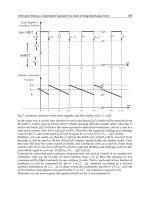
4.3 Uncertainty and business model increase
When using (as a comparison basis) the total backlog values of the scenarios with
uncertainty and business model equal to 0, we found that higher (or equal) total backlog
values are found more frequently than lower values when there is a mismatch between the
level of demand uncertainty present and the business model used to cope with it (lower left
quadrant and upper right quadrant of Figure 6). An interesting fact is the role played by
uncertainty in this mismatch: when uncertainty is low, 100% of the time higher (or equal)
total backlog values are found (lower left quadrant of Figure 6). But when uncertainty is
total then lower total backlog values can be found (lower right quadrant of Figure 6). This
suggests that as the level of uncertainty increases, lower total backlog values are to be found
(independently of the level of business model used).


bm u = 0 u = 0.25 u = 0.5 u = 0.75 u = 1

0





0.25





0.5





0.75





1

reference lower values than reference higher values than reference

Fig. 6. Comparison of scenarios, uncertainty and business model values increase
Quantifying the Demand Fulfillment Capability of a Manufacturing Organization

483
In fact, when using the scenarios with a business model level of zero as a comparison basis,
an analysis of Tables 4, 5, and 6 reveals the same behavior: within the same level of
uncertainty, all the different business model levels (i.e. bm = 0, 0.25, 0.5, etc.), present the
same the total backlog values behavior. In this way, for an uncertainty level of:
• 0; total backlog values decrease 0% of the time, remain the same 36% of the time, and
increase 64% of the time.
• 0.25; total backlog values decrease 32% of the time, remain the same 16% of the time,
and increase 52% of the time.
• 0.5; total backlog values decrease 40% of the time, remain the same 20% of the time, and
increase 40% of the time.
• 0.75; total backlog values decrease 52% of the time, remain the same 16% of the time,
and increase 32% of the time.
• 1.0; total backlog values decrease 64% of the time, remain the same 36% of the time,
and increase 0% of the time.
4.4 Total backlog values frequency
When the values of Tables 4, 5, and 6 are classified according to the frequency a value
appears within certain range, we found that:
• The distribution of the values is symmetrical (for the most part). This behavior has to do
with the assumption that there is a continuum betwen the contributions made to
demand fulfillment, by the inventory and the capacity strategies, Equations (1) and (2).
Total backlog values can be obtained through different combinations of u, bm, s, and f
(Table 7), i.e. eight total backlog values in the range of 2,000 – 3,000.

Value range frequency frequency %
10000+ 62 9.76
9000-10000 314 50.4
8000-9000 134 21.6
7000-8000 52 8.32
6000-7000 26 4.16
5000-6000 16 2.56
4000-5000 12 1.76
2000-3000 8 1.28
0-1000 2 0.16

Table 7. Total backlog values frequency
4.5 Implications for the automotive SC partner
As the level of uncertainty can not be controlled by the automotive SC partner, this last has to
focus in adjusting the levels of standardization and/or flexibility rather than in adjusting the
level of business model: while a total match between the business model used an the level of
uncertainty present is not a guarantee of 100% lower total backlog values, neither a total
mismatch guarantee 100% higher total backlog values. In fact, [38] reports that the
standardization of a small number of semi-finished products resulted in a large reduction in
the average lead times and with this, the increasing of volume of customer orders that can be
processed during a certain period of volatile demand. If we take into account that a business
Supply Chain Management

484
model can be understood in terms of its level of customer feedback [23], i.e. all the activities in
a pure MTO environment are driven by customer’s information (so uncertainty of what to do
next, when to do it, and for how long to do it, is at its maximum), then further research is
called in the area of optimum customer feedback (that is, the level of customer feedback
information with the least cost that allows the maximum reduction of the total backlog value).
A second implication is related to the frequency of the total backlog values: the automotive

SC partner should follow and adaptive strategy in the management of its operations, as the
same total backlog values can be obtained through different combinations of uncertainty,
business model, standardization, and flexibility. Therefore, it is necessary to not only
determine the optimum level customer feedback (as proposed earlier), but also the range of
matchness (between uncertainty and the business model used) that would allow achieving a
high frecuency of lower total backlog values, in the event of dealing with a high varying
environment.
5. Conclusions
Manufacturing enterprises are pressured to shift from the traditional MTS to the MTO
production model, and at the same time, compete against each other as part of a SC, in order to
respond to changes in the customers’ demands. As the decisions taken at the strategic level of
the SC have a deep impact at the operational level of the manufacturing organization, it
becomes necessary the alignment of activities, from the strategic level through the
operational level. The objective of this paper was to quantitatively evaluate the impact of such
alignment of the total backlog value of a manufacturing organization. For this reason, an
analytical expression was derived a system dynamics (SD) simulation model was developed
and tested under different scenarios (in order to collect statistical data regarding total backlog).
The usefulness of the analytical expression was illustrated via a case study of an automotive
SC partner and conclusions were derived regarding actions to improve its demand fulfillment
capability. This research effort acknowledges that the misalignment between the strategic and
operational levels creates an obstacle to demand fulfillment: the bigger the misalignment is,
the bigger the obstacle to achieve the demanded volume will be. This idea resembles the
concept of structural complexity proposed by [39], whom states that a high level of complexity
in the structure of a production system (i.e. the number of operations and machines present in
the routing sheets of a product family), has the effect of building obstacles that impedes the
process flow. Future research will explore this venue and also, the use of a simulation-by-
optimization approach (that is, finding out values of the decision variables which optimize a
quantitative objective function under constraints).
6. References
[1] Ismail, H.S., Sharifi, H., A balanced approach to building agile supply chains,

International Journal of Physical Distribution & Logistics Management 36 (6) (2006)
431-444.
[2] Duclos, L., Vokurka, R., Lummus, R. A conceptual model of supply chain flexibility,
Industrial Management & Data Systems 103 (6) (2000) 446-456.
[3] Terzi, S., Cavalieri, S. Simulation in the supply chain context: a survey, Computers in
Industry 53 (2004) 3–16.
[4] Ngai, E.W.T., Gunasekaran, A. Build-to-order supply chain management: a literature
review and framework for development, Journal of Operations Management 23
(2005) 423–451.
Quantifying the Demand Fulfillment Capability of a Manufacturing Organization

485
[5] Li, D., O’Brien, C. 1999. Integrated decision modeling of supply chain efficiency,
International Journal of Production Economics 59 (1999) 147-157.
[6] Li, D., O’Brien, C. A quantitative analysis of relationships between product types and
supply chain strategies, International Journal of Production Economics 73 (2001) 29-
39.
[7] Vonderembse, M.A., Uppal, M., Huang, S.H., Dismukes, J.P. Designing supply chains:
Towards theory development, International Journal of Production Economics 100
(006) 223–238.
[8] Olhager, J. Strategic positioning of the order penetration point, International Journal of
Production Economics 85 (3) (2003) 2335-2351.
[9] Vernadat, F. UEML: towards a unified enterprise modeling language, International
Journal of Production Research 40 (17) (2002) 4309-4321.
[10] Angelides, M.C., Angerhofer, B.J. A model and a performance measurement system for
collaborative supply chains, Decision Support Systems 42 (2006) 283– 301.
[11] Son, Y.J., Venkateswaran, J. Hybrid system dynamic: discrete event simulation-based
architecture for hierarchical production planning, International Journal of
Production Research 43 (20) (2005) 4397–4429.
[12] Khoo, L.P., Yin, X.F. An extended graph-based virtual clustering-enhanced approach to

supply chain optimization, International Journal of Advanced Manufacturing
Technology 22 (2003) 836–847.
[13] Zhang, D.Z., Anosike, A.I., Lim, M.K., Akanle,O.M. An agent-based approach for e-
manufacturing and supply chain integration, Computers & Industrial Engineering
51 (2006) 343–360.
[14] Martinez-Olvera, C., Shunk, D. A comprehensive framework for the development of a
supply chain strategy, International Journal of Production Research 44 (21) (2006)
4511–4528.
[15] Griffiths, J., James, R., Kempson, J. Focusing customer demand through manufacturing
supply chains by the use of customer focused cells: an appraisal. International
Journal of Production Economics 65 (1) (2000) 111-120.
[16] Chibba, A., Ake Horte, S., Supply chain performance – A Meta Analysis, European
operations management association & Production and operations management
society, Joint conference, June, 16-18 (2003).
[17] Gunasekaran, A., Patelb, C., McGaughey, R.E. A framework for supply chain
performance measurement, International Journal of Production Economics 87
(2004) 333–347.
[18] Chen, C., C. An objective-oriented and product-line-based manufacturing performance
measurement, International Journal of Production Economics 112 (2008) 380–390.
[19] Safizadeh, M.H., Ritzman, L.P. Linking performance drivers in production planning
and inventory control to process choice, Journal of Operations Management 15
(1997) 389-403
[20] Gupta, D., Benjaafar, S. Make-to-order, make-to-stock, or delay product differentiation?
A common framework for modeling and analysis, IIE Transactions 36 (2004) 529–
546.
[21] Buxey, G. Strategy not tactics drives aggregate planning, International Journal of
Production Economics 85 (2003) 331–346.
[22] Miltenburg, J. Manufacturing Strategy: How to Formulate and Implement a Winning
Plan, Productivity Press, Portland, Oregon (1995).
Supply Chain Management

486
[23] Martinez-Olvera, C. Impact of hybrid business models in the supply chain performance,
book chapter. Supply Chain: Theory and Applications, ISBN 978-3-902613-22-6. I-
Tech Education and Publishing, Vienna, Austria, European Union (2008a).
[24] Martinez-Olvera, C. Methodology for realignment of supply-chain structural,
International Journal of Production Economics, doi:10.1016/j.ijpe.2008.03.008
(2008b),
[25] Huang, S.H., Uppal, M., Shi, J. A product driven approach to manufacturing supply
chain selection, Supply chain management 7 (4) (2002) 189-199.
[26] Shah, N., Hung, W.Y., Kucherenko, S., Samsatli, N.J. A flexible and generic approach to
dynamic modelling of supply chains, Journal of the Operational Research Society
55 (2004) 801–813.
[27] Towill, D.R. Time compression and supply chain management – a guided tour. Supply
chain management 1 (1) (1996) 15-27.
[28] Venkateswaran, J., Son, Y. J. Impact of modeling approximations in supply chain
analysis – an experimental study, International Journal of Production Research 42
(15) (2004) 2971–2992.
[29] Zhao, Z.Y., Ball, M., Chen, C.Y. A scalable supply chain infrastructure research test-bed.
Department of decision & information technology. Robert H. Smith, School of
Business, University of Maryland (2002).
[30] Longo, F., Mirabelli, G. An advanced supply chain management tool based on modeling
and simulation, Computers & Industrial Engineering 54 (2008) 570–588.
[31] Roder, A., Tibken, B. A methodology for modeling inter-company supply chains and for
evaluating a method of integrated product and process documentation, European
Journal of Operational Research 169 (2006) 1010–1029.
[32] Huang, M., Ip, W.H., Yung, K.L., Wang, X., Wang, D. Simulation study using system
dynamics for a CONWIP-controlled lamp supply chain, International Journal of
Advanced Manufacturing Technology 32 (2007) 184–193. DOI 10.1007/s00170-005-
0324-2

[33] Kleijnen, J.P.C. Supply chain simulation tools and techniques: a survey, International
Journal of Simulation & Process Modelling 1 (1/2) (2005) 82-89.
[34] Eskandari, H., Rabelo, L., Shaalan, T., Helal, M. Value chain analysis using hybrid
simulation and AHP, International Journal of Production Economics 105 (2007)
536–547.
[35] iThink Analyst Technical Documentation, High Performance Systems, Inc. (1996)
[36] Hwarng, H. B., Chong, C. S. P., Xie, N., Burgess, T.F., 2005. Modeling a complex supply
chain: understanding the effect of simplified assumptions, International Journal of
Production Research 43 (13) (2005) 2829–2872.
[37] Banks, J. Discrete-event system simulation, Upper Saddle River, NJ : Prentice Hall.
(2000)
[38] Kuroda, M., Mihira, H. Strategic inventory holding to allow the estimation of earlier
due dates in make-to-order production, International Journal of Production
Research 46 (2) (2008) 495–508.
[39] Frizelle, G., Woodcock, E. Measuring complexity as an aid to developing strategy,
International Journal of Operations & Production Management 15 (5) (1995) 268-
270.
1. Introduction
A supply network consists of suppliers, manufacturers, warehouses, and stores, that perform
the functions of materials procurement, their transformation into intermediate and finished
goods, and the distribution of the final products to customers among different production
facilities. Mathematical models are used to monitor cost-efficient distribution of parts and
to measure current business processes. The main aim is to plan supply networks so as to
reduce the dead times and to avoid bottlenecks, obtaining as a result a greater coordination
leading to the optimization of the production process of a given good. Several questions arise
in the design of optimal supply chain networks: can we control the maximum processing
rates, or the processing velocities, or the input flow in such way to minimize the value the
queues attain and to achieve an expected outflow? The formulation of optimization problems
for supply chain management is an immediate consequence of performing successful supply
modeling and hence simulations.

Depending on the scale, supply networks modelling is characterized by different
mathematical approaches: discrete event simulations and continuous models. Since
discrete event models are based on considerations of individual parts, the principal
drawback of them, however, is their enormous computational effort. A cost-effective
alternative to discrete event models is continuous models (e.g. for models based on
ordinary differential equations see Daganzo (2003), Helbing et al. (2004), Nagatani & Helbing
(2004), Helbing & L¨ammer (2005), Helbing et al. (2006)), in particular fluid-like network
models using partial differential equations describing averaged quantities like density and
average velocity (see Armbruster et al. (2004), G ¨ottlich et al. (2005), Armbruster et al. (2006a),
Armbruster et al. (2006b), Armbruster et al. (2006c), G¨ottlich et al. (2006), Herty et al. (2007),
D’Apice et al. (2010)). Probably the first paper for supply chains in continuous direction was
Armbruster et al. (2006b) where the authors, taking the limit on the number of parts and
suppliers, have obtained a conservation law, whose flux is described by the minimum among
the parts density and the maximal productive capacity.
Due to the difficulty of finding solution for the general equation proposed in Armbruster et al.
(2006b), other fluid dynamic models for supply chains were introduced in G¨ottlich et al.
(2005), D’Apice & Manzo (2006) and Bretti et al. (2007).
Ciro D’Apice
1
, Rosanna Manzo
1
and Benedetto Piccoli
2
1
Department of Information Engineering and Applied Mathematics
University of Salerno, Fisciano (SA)
2
Department of Mathematical Sciences, Rutgers University - Camden, Camden, NJ
1
Italy

2
United States

Continuum-Discrete Models
for Supply Chains and Networks
23
2 Supply Chain Coordination and Management
The work D’Apice & Manzo (2006) is based on a mixed continuum-discrete model, i.e. the
supply chain is described by a graph consisting of consecutive arcs separated by nodes. The
arcs represent processors or sub-chains, while the nodes model connections between arcs at
which the dynamics can be regulated. The chain load, expressed by the part density and
the processing rate, follows a time-space continuous evolution on arcs, and at nodes the
conservation of the goods density is imposed, but not of the processing rate. In fact, on
each arc an hyperbolic system of two equations is considered: a conservation law for the
goods density, and a semi-linear evolution equation for the processing rate. At nodes a
way to solve Riemann Problems, i.e. Cauchy problems with constant initial data on each
arc, is prescribed and a solution at nodes guaranteeing the conservation of fluxes is defined.
Moreover, existence of solutions to Cauchy problems was proved.
The paper G¨ottlich et al. (2005) deals with a conservation law, with constant processing rate,
inside each supply sub-chain, with an entering queue for exceeding parts. The dynamics at a
node is solved considering an ode for the queue. Some optimization technique for the model
described in G¨ottlich et al. (2005) is developed in G¨ottlich et al. (2006), while the existence
of solutions to Cauchy problems with the front tracking method is proved in Herty et al.
(2007). In particular in G¨ottlich et al. (2006) the question of optimal operating velocities for
each individual processing unit is treated for a supply chain network consisting of three
processors. The maximal processing rates are fixed and not subject to change. The controls
are the processing velocities. Given some default initial velocities the processing velocities
are found to minimize the height of the buffering queues and producing a certain outflow.
Moreover given a supply chain network with a vertex of dispersing type, the distribution rate
has been controlled in such way to minimize the queues.

It is evident that the models described in G¨ottlich et al. (2005) and D’Apice & Manzo (2006)
complete each other. In fact, the approach of G¨ottlich et al. (2005) is more suitable when
the presence of queue with buffer is fundamental to manage goods production. The model
of D’Apice & Manzo (2006), on the other hand, is useful when there is the possibility to
reorganize the supply chain: in particular, the productive capacity can be readapted for some
contingent necessity.
Starting from the model introduced in D’Apice & Manzo (2006) and fixing the rule that
the objects are processed in order to maximize the flux, two different Riemann Solvers
are defined and equilibria at a node are discussed in Bretti et al. (2007). Moreover,
discretization algorithms to find approximated solution to the problem are described,
numerical experiments on sample supply chains are reported and discussed for both the
Riemann Solvers.
In D’Apice et al. (2010) existence of solutions to Cauchy problems is proven for both
continuum-discrete supply chains and networks models, deriving estimates on the total
variation of the density flux, density and processing rate along a wave-front tracking
approximate solution.
Observe that while the papers Armbruster et al. (2006b), D’Apice & Manzo (2006), Bretti et al.
(2007) treat the case of chains, i.e. sequential processors, modelled by a real line seen as a
sequence of sub-chains corresponding to real intervals, the model in G¨ottlich et al. (2005) and
the extended results in G¨ottlich et al. (2006), Herty et al. (2007), D’Apice et al. (2009) refer to
networks.
In this Chapter we describe the continuum-discrete models for supply chains and networks
reporting the main results of D’Apice & Manzo (2006), Bretti et al. (2007) and D’Apice et al.
(2009).
488
Supply Chain Management
Continuum-Discrete Models for Supply Chains and Networks 3
We recall the basic supply chain model under consideration: a supply chain consists of
sequential processors or arcs which are going to assemble and construct parts. Each processor
is characterized by a maximum processing rate μ

e
, its length L
e
and the processing time T
e
.
The rate L
e
/T
e
represents the processing velocity.
The supply chain is modelled by a real line seen as a sequence of arcs corresponding to real
intervals
[
a
e
,b
e
]
such that
[
a
e
,b
e
]
∩

a
e+1

,b
e+1

= v
e
: a node separating arcs. The dynamic of
each arc is governed by a continuum system of the type
ρ
t
+ f
ε
(ρ, μ)
x
= 0,
μ
t
−μ
x
= 0,
where ρ
(t, x) ∈ [0, ρ
max
] is the density of objects processed by the supply chain at point x and
time t and μ
(t, x) ∈ [0, μ
max
] is the processing rate. For ε > 0, the flux f
ε
is given by:
f

ε
(ρ, μ)=

m ρ,ifρ
≤ μ,
m μ
+ ε(ρ −μ),ifρ ≥ μ,
where m is the processing velocity.
The evolution at nodes v
e
has been interpreted thinking to it as Riemann Problems for the
density equation with μ data as parameters. Keeping the analogy to Riemann Problems, we
call the latter Riemann Solver at nodes. In D’Apice & Manzo (2006) the following rule was
used:
SC1 The incoming density flux is equal to the outgoing density flux. Then, if a solution with
only waves in the density ρ exists, then such solution is taken, otherwise the minimal μ
wave is produced.
Rule SC1 corresponds to the case in which processing rate adjustments are done only if
necessary, while the density ρ can be regulated more freely. Thus, it is justified in all situations
in which processing rate adjustments require re-building of the supply chain, while density
adjustments are operated easily (e.g. by stocking). Even if rule SC1 is the most natural also
from a geometric point of view, in the space of Riemann data, it produces waves only to
lower the value of μ. As a consequence in some cases the value of the processing rate does
not increase and it is not possible to maximize the flux. In order to avoid this problem two
additional rules to solve dynamics at a node have been analyzed in Bretti et al. (2007):
SC2 The objects are processed in order to maximize the flux with the minimal value of the
processing rate.
SC3 The objects are processed in order to maximize the flux. Then, if a solution with only
waves in the density ρ exists, then such solution is taken, otherwise the minimal μ wave
is produced.

The continuum-discrete model, regarding sequential supply chains, has been generalized to
supply networks which consist of arcs and two types of nodes: nodes with one incoming arc
and more outgoing ones and nodes with more incoming arcs and one outgoing arc.
The Riemann Problems are solved fixing two “routing” algorithms:
RA1 Goods from an incoming arc are sent to outgoing ones according to their final
destination in order to maximize the flux over incoming arcs. Goods are processed
ordered by arrival time (FIFO policy).
489
Continuum-Discrete Models for Supply Chains and Networks
4 Supply Chain Coordination and Management
RA2 Goods are processed by arrival time (FIFO policy) and are sent to outgoing arcs in order
to maximize the flux over incoming and outgoing arcs.
For both routing algorithms the flux of goods is maximized considering one of the two
additional rules, SC2 and SC3.
In order to motivate the introduction of the model and to understand the mechanism of the
above rules, we show some examples of real supply networks.
We analyze the behaviour of a supply network for assembling pear and apple fruit juice
bottles, whose scheme is in Figure 1 (left).
Bottles coming from arc e
1
are sterilized in node v
1
. Then, the sterilized bottles, with a certain
probability α are directed to node v
3
, where apple fruit juice is bottled, and with probability
1
− α to node 4, where the pear fruit juice is bottled. In nodes v
5
and v

6
, bottles are labelled.
Finally, in node 7, produced bottles are corked. Assume that pear and apple fruit juice bottles
are produced using two different bottle shapes. The bottles are addressed from arc e
2
to
the outgoing sub-chains e
3
and e
4
in which they are filled up with apple or pear fruit juice
according to the bottle shape and thus according to their final destination: production of apple
or pear fruit juice bottles. In a model able to describe this situation, the dynamics at node v
2
is solved using the RA1 algorithm. In fact, the redirection of bottles in order to maximize the
production on both incoming and outgoing sub-chains is not possible, since bottles with apple
and pear fruit juice have different shapes.
Consider a supply network for colored cups (Figure 1, right). The white cups are addressed
towards n sub-chains in which they are colored using different colors. Since the aim is to
maximize the cups production independently from the colors, a mechanism is realized which
addresses the cups on the outgoing sub-chains by taking into account their loads in such
way as to maximize flux on both incoming and outgoing sub-chains. It follows that a model
realized to capture the behavior of the described supply network is based on rule RA2.
Let us now analyze an existing supply network where both algorithms shows up naturally:
the chips production of the San Carlo enterprise. The productive processes follows various
steps, that can be summarized in this way: when potatoes arrive at the enterprise, they are
subjected to a goodness test. After this test, everything is ready for chips production, that
starts with potatoes wash in drinking water. After washing potatoes, they are skinned off,
rewashed and subjected to a qualification test. Then, they are cut by an automatic machine,
and, finally, washed and dried by an air blow. At this point, potatoes are ready to be fried in

vegetable oil for some minutes and, after this, the surplus oil is dripped. Potatoes are then
salted by a dispenser, that nebulizes salt spreading it on potatoes. An opportune chooser
Α
 Α
$
$
3
3

Y

Y

Y

Y

Y

Y

Y

H

H

H

H


H

H

H

H

H
Fig. 1. Fruit juice network and cups production.
490
Supply Chain Management
Continuum-Discrete Models for Supply Chains and Networks 5
Fig. 2. Graph of the supply network for chips production (top) and possible arcs (bottom).
is useful to select the best products. The final phase of the process is given by potatoes
confection. A simplified vision of the supply chain network is in Fig. 2 (top).
In phases 1, 5 and 10 a discrimination is made in production in order to distinguish good and
bad products. In such sense, we can say that there is a statistical percentage α of product, that
follows the production steps, while the percentage 1
−α is the product discarded (obviously,
the percentage α can be different for different phases). Therefore, the goods routing in these
nodes follows the algorithm RA1. On the other side, phase 6 concerns the potatoes cut: as the
enterprise produces different types of fried potatoes (classical, grill, light, stick, etc.), different
ways of cutting potatoes must be considered. Assume that, for simplicity, there are only
two types of potatoes production, then the supply network is as in Fig. 2 (bottom). If the
aim is only the production maximization independently from the type, then the potatoes are
addressed from node 6 towards the outgoing arcs according to the RA2 algorithm.
The Chapter is organized as follows. Section 2 is devoted the description of the
continuum-discrete model for supply chain. In particular Subsection 2.1 gives the basic

definitions of supply chain and Riemann Solver. Then the dynamics inside an arc is studied.
In Subsection 2.2 particular Riemann Solvers according to rules SC1, SC2 and SC3 are defined
and explicit unique solutions are given. Moreover test simulations are reported. Section 3
extends the model to simple supply networks.
491
Continuum-Discrete Models for Supply Chains and Networks
6 Supply Chain Coordination and Management
2. A continuum-discrete model for supply chains
In this Section we present a model able to describe the load dynamics on supply chains, i.e.
sequential processors, modelled by a real line seen as a sequence of sub-chains corresponding
to real intervals.
2.1 Basic definitions
We start from the conservation law model of Armbruster et al. (2006b):
ρ
t
+(min{μ(t, x), ρ})
x
= 0. (1)
To avoid problems of existence of solutions, we assume μ piecewise constant and an evolution
equation of semi-linear type:
μ
t
+ Vμ
x
= 0, (2)
where
V is some constant velocity. Taking V = 0, we may have no solution to a Riemann
Problem for the system (1)–(2) with data
(ρ
l

,μ
l
) and (ρ
r
,μ
r
) if min{μ
l
,ρ
l
} > μ
r
.Sincewe
expect the chain to influence backward the processing rate we assume
V < 0 and for simplicity
we set
V = −1.
We define a mixed continuum-discrete model in the following way. On each arc e,the
evolution is given by (1)–(2). On the other side, the evolution at nodes v
e
is given solving
Riemann Problems for the density equation (1) with μs as parameters. Such Riemann
Problems may still admit no solution as before if we keep the values of the parameters μs
constant, thus we expect μ waves to be generated and then follow equation (2). The vanishing
of the characteristic velocity for (1), in case ρ
> μ, can provoke resonances with the nodes
(which can be thought as waves with zero velocities). Therefore, we slightly modify the model
as follows.
Each arc e is characterized by a maximum density ρ
e

max
, a maximum processing rate μ
e
max
and
aflux f
e
ε
.Forafixedε > 0, the dynamics is given by:

ρ
t
+ f
e
ε
(ρ, μ)
x
= 0,
μ
t
−μ
x
= 0.
(3)
The flux is defined as:
(F) f
e
ε
(
ρ, μ

)
=

ρ,0
≤ ρ ≤ μ,
μ
+ ε(ρ −μ), μ ≤ ρ ≤ ρ
e
max
,
f
e
ε
(
ρ, μ
)
=

ερ
+(1 − ε)μ,0≤ μ ≤ ρ,
ρ, ρ
≤ μ ≤ μ
e
max
,
see Figure 3.
The conservation law for the good density in (3) is a ε perturbation of (1) in the sense that
f − f
ε


∞
≤Cε,where f is the flux of (1). The equation has the advantage of producing waves
with always strictly positive speed, thus avoiding resonance with the “boundary”problems at
nodes v
e
.
Remark 1 We can consider a slope m, defining the flux
f
ε
(ρ, μ)=

m ρ,ifρ
≤ μ,
m μ
+ ε(ρ −μ),ifρ ≥ μ,
(4)
492
Supply Chain Management
Continuum-Discrete Models for Supply Chains and Networks 7
Μ
fΡ

,Μ
Ρ

Μ
max
e
Ρ


 Ρ

Ρ
fΡ,Μ


Μ

Ρ
max
e
Μ

Μ

Ρ
max
e
Μ


Fig. 3. Flux (F): Left, f (
¯
ρ, μ
).Right,f(ρ,
¯
μ).
or different slopes m
e
, considering the flux

f
e
ε
(
ρ, μ
)
=

m
e
ρ,0≤ ρ ≤ μ,
m
e
μ + ε(ρ −μ), μ ≤ ρ ≤ ρ
e
max
,
(5)
where m
e
≥ 0 represents the velocity of each processor and is given by m
e
=
L
e
T
e
,withL
e
and T

e
,
respectively, fixed length and processing time of processor e.
From now on, for simplicity we assume that ε is fixed and the flux is the same for each arc
e, we then drop the indices thus indicate the flux by f
(ρ, μ). The general case can be treated
similarly.
The supply chain evolution is described by a finite set of functions ρ
e
,μ
e
defined on
[
0, +∞
[
×
[
a
e
,b
e
].Oneachsub-chain[a
e
,b
e
], we say that U
e
:=(ρ
e
,μ

e
) :
[
0, +∞
[
× [
a
e
,b
e
] → R is a weak
solution to (3) if, for every C
∞
-function ϕ :
[
0, +∞
[
× [
a
e
,b
e
] → R
2
with compact support in
]
0, +∞
[
×
]

a
e
,b
e
[
,
+∞

0
b
e

a
e

U
e
·
∂ϕ
∂t
+ f (U
e
) ·
∂ϕ
∂x

dxdt
= 0,
where
f

(U
e
)=

f
(ρ
e
,μ
e
)
−
μ
e

,
is the flux function of the system (3). For the definition of entropy solution, we refer to Bressan
(2000).
For a scalar conservation law, a Riemann Problem (RP) is a Cauchy problem for an initial
data of Heavyside type, that is piecewise constant with only one discontinuity. One looks
for centered solutions, i.e. ρ
(t, x)=φ(
x
t
) formed by simple waves, which are the building
blocks to construct solutions to the Cauchy problem via wave- front tracking algorithm. These
solutions are formed by continuous waves called rarefactions and by travelling discontinuities
called shocks. The speed of waves are related to the values of f

, see Bressan (2000).
Analogously, we call Riemann Problem for a junction the Cauchy problem corresponding to

an initial data which is constant on each supply line.
Definition 2 A Riemann Solver for the node v
e
consists in a map RS :
[0, ρ
e
max
] × [0, μ
e
max
] × [0, ρ
e+1
max
] × [0, μ
e+1
max
] → [ 0, ρ
e
max
] × [0, μ
e
max
] × [0, ρ
e+1
max
] ×
[
0, μ
e+1
max

] that associates to a Riemann data ( ρ
e,0
,μ
e,0
,ρ
e+1,0
,μ
e+1,0
) at v
e
avector
493
Continuum-Discrete Models for Supply Chains and Networks
8 Supply Chain Coordination and Management
(
ˆ
ρ
e
,
ˆ
μ
e
,
ˆ
ρ
e+1
,
ˆ
μ
e+1

) so that the solution is given by the waves (ρ
e,0
,
ˆ
ρ
e
) and (μ
e,0
,
ˆ
μ
e
) on the
arc e and by the waves
(
ˆ
ρ
e+1
,ρ
e+1,0
),and(
ˆ
μ
e+1
,μ
e+1,0
) on the ar c e + 1. We require the consistency
condition
(CC) RS
(RS(ρ

e,0
,μ
e,0
,ρ
e+1,0
,μ
e+1,0
)) = RS((ρ
e,0
,μ
e,0
,ρ
e+1,0
,μ
e+1,0
)).
Once a Riemann Solver is assigned we can define admissible solutions at v
e
.
Definition 3 Assume a Riemann Solver RS is assigned for the node v
e
.LetU=(U
e
,U
e+1
) be such
that U
e
(t, ·) and U
e+1

(t, ·) are of bounded variation for every t ≥ 0. Then U is an admissible weak
solution of (3) related to RS at the junction v
e
if and only if the following property holds for almost
every t. Setting

U
e
(t)=(U
e
(·, b
e
−),U
e+1
(·, a
e
+))
we have RS(

U
e
(t)) =

U
e
(t).
Our aim is to solve the Cauchy problem for t
≥ 0 for given initial data.
2.1.1 Dynamics on arcs
Let us fix an arc e and analyze system (3): it is a system of conservation laws in the variables

U
=(ρ, μ):
U
t
+ F(U)
x
= 0, (6)
with flux function given by F
(U)=(f(ρ, μ), −μ), thus the Jacobian matrix of the flux is:
DF
(ρ, μ)=
⎧
⎪
⎪
⎪
⎪
⎨
⎪
⎪
⎪
⎪
⎩

10
0
−1

,ifρ
< μ,


ε 1
−ε
0
−1

,ifρ
> μ.
The eigenvalues and eigenvectors are given by:
λ
1
(ρ, μ)=−1, r
1
(ρ, μ)=
⎧
⎪
⎪
⎪
⎪
⎨
⎪
⎪
⎪
⎪
⎩

0
1

,ifρ
< μ,


−
1−ε
1+ε
1

,ifρ
> μ,
λ
2
(ρ, μ)=

1, if ρ
< μ,
ε,ifρ
> μ,
r
2
(ρ, μ)=

1
0

.
Hence the Hugoniot curves for the first family are vertical lines above the secant ρ
= μ and
lines with slope close to
−1/2 below the same secant. The Hugoniot curves for the second
family are just horizontal lines. Since we consider positive and bounded values for the
variables, we fix the invariant region:

D = {(ρ, μ) :0≤ ρ ≤ ρ
max
,0≤ μ ≤ μ
max
,
0
≤ (1 + ε)ρ +(1 −ε)μ ≤ (1 + ε)ρ
max
= 2( 1 − ε)μ
max
}
494
Supply Chain Management
Continuum-Discrete Models for Supply Chains and Networks 9
Ρ
Μ
PPΡ
max
Μ
max
Ρ,Μ
Ρ,Μ
ΡΜ
1st family curve
1st family curve
2nd family curve
2nd family curve
Fig. 4. First and second family curves.
see Figure 4.
Observe that

ρ
max
= μ
max
2
1 + ε
.(7)
Proposition 4 Given
(ρ
0
,μ
0
), the minimal value of the flux at points of the curve of the first family
passing through
(ρ
0
,μ
0
) is given by:
f
min
((ρ
0
,μ
0
)) =

2ε
1+ε
ρ

0
, if ρ
0
≤ μ
0
,
ερ
0
+
ε(1−ε)
1+ε
μ
0
, if ρ
0
> μ
0
.
Lemma 5 Given an initial datum
(ρ
0
,μ
0
), the maximum value of the density of the curve of the second
family passing through
(ρ
0
,μ
0
) and belonging to the invariant region is given by

ρ
M
(μ
0
)=ρ
max
−μ
0
ρ
max
−μ
max
μ
max
.(8)
2.2 Riemann Solvers at nodes
In this Section we discuss possible definitions of a general Riemann Solver, which conserves
the flux at nodes. We fix a node v
e
and a Riemann initial datum: constantly equal to (ρ
e,0
,μ
e,0
)
on e and constantly equal to (ρ
e+1,0
,μ
e+1,0
) on e + 1.
First observe that the following Lemmas hold:

Lemma 6 On the incoming arc, only waves of the first family may be produced, while on the outgoing
arc only waves of the second family may be produced.
Lemma 7 The Riemann Problem at node v
e
admits a solution if the following holds.
If ρ
e,0
≤ μ
e,0
then
μ
e+1,0
(1 −ε)+ε(ρ
e+1
max
−
2
1 + ε
ρ
e,0
) ≥ 0. (9)
495
Continuum-Discrete Models for Supply Chains and Networks