Advanced Topics in Mass Transfer Part 8 pot

Simulation of Hydrodynamics and Mass Transfer
in a Valve Tray Distillation Column Using Computational Fluid Dynamics Approach

269
where K
pq
( K
qp
) is the interphase momentum exchange coefficient; and it tends to zero
whenever the primary phase is not present within the domain.
In simulations of the multiphase flow, the lift force can be considered for the secondary
phase (gas). This force is important if the bubble diameter is very large. It was assumed that
the bubble diameters were smaller than the distance between them, so the lift force was
insignificant compared with the other forces, such as drag force. Therefore, there was no
reason to include this extra term.
The exchange coefficient for these types of gas-liquid mixtures can be written in the
following general form:

qpp
pq
p
f
K
α
αρ
τ
= (6)
where
f
and
p

τ
are the drag function and relaxation time, respectively.
f
can be defined
differently for the each of the exchange-coefficient models. Nearly all definitions of
f

include a drag coefficient that is based on the relative Reynolds number. In this study the
basic drag correlation implemented in FLUENT (
Schiller-Naumann) was used in order to
predict the drag coefficient.
In comparison with single-phase flows, the number of terms to be modeled in the
momentum equations in multiphase flows is large, which complicates the modeling of
turbulence in multiphase simulations.
In the present study, standard
k -
ε
turbulence model was used. The simplest "complete
models" of turbulence are two-equation models in which the solution of two separate
transport equations allows the turbulent velocity and length scales to be independently
determined. Eeconomy, and reasonable accuracy for a wide range of turbulent flows explain
popularity of the standard
k -
ε
model in industrial flow and heat transfer simulations. It is
a semi-empirical model, and the derivation of the model equations relies on
phenomenological considerations and empiricism (FLUENT 6.2 Users Guide, 2005).
The equations
k and
ε

that describe the model are as follows:

,
,
().( ).( )
tm
mmm kmm
k
kvk kG
t
μ
ρ
ρρε
σ
∂
+∇ =∇ ∇ + −
∂
G
(7)
and

,
1, 2
().( ).( )( )
tm
mmm kmm
vCGC
tk
εε
ε

μ
ε
ρ
ερε ε ρε
σ
∂
+∇ =∇ ∇ + −
∂
G
(8)
where
k and
ε
shows turbulent kinetic energy and dissipation rate, respectively; and
1
C
ε
,
2
C
ε
,
k
σ
and
σ
ε
are parameters of the model. The mixture density and velocity,
m
ρ

and v
m
G
, are computed from:

1
N
mii
i
ρ
αρ
=
=
∑
(9)
and
Advanced Topics in Mass Transfer

270

1
1
N
iii
i
m
N
ii
i

v
v
α
ρ
α
ρ
=
=
=
∑
∑
G
G
(10)
The turbulent viscosity
,
tm
μ
is computed from:

2
,tm m
k
C
μ
μρ
ε
= (11)
The production of turbulent kinetic energy
,

G
km
is computed from:

,,
(()):
T
km tm m m m
Gvvv
μ
=
∇+∇ ∇
G
GG
(12)
2.2 Species transport equations
To solve conservation equations for chemical species, software predicts the local mass
fraction of each species,
Y
i
, through the solution of a convection-diffusion equation for the i
th

species. This conservation equation takes the following general form:

() ( )
ii ii
YvYjRS
t
ρρ

∂
+
∇⋅ =−∇⋅ + +
∂
(13)
where
R
i
is the net rate of production of species i by chemical reaction and here it is zero. S
i

is the rate of creation by addition from the dispersed phase plus any user-defined sources.
An equation of this form will be solved for N -1 species where N is the total number of fluid
phase chemical species present in the system. Since the mass fraction of the species must
sum to unity, the Nth mass fraction is determined as one minus the sum of the N - 1 solved
mass fractions.
In Equation (13),
J
i
is the diffusion flux of species i, which arises due to concentration
gradients. By default, FLUENT uses the dilute approximation, under which the diffusion
flux can be written as:

Ji = -
ρ
D
i,m
i
Y
∇

(14)
Here D
i,m
is the diffusion coefficient for species i in the mixture.
3. Numerical implementation
3.1 Simulation characteristics
In the present work, commercial grid-generation tools, GAMBIT 2.2 (FLUENT Inc., USA)
and CATIA were used to create the geometry and generate the grids. The use of an adequate
number of computational cells while numerically solving the governing equations over the
solution domain is very important. To divide the geometry into discrete control volumes,
more than 5.7×10
5
3-D tetrahedral computational cells and 37432 nodes were used.
Schematic of the valve tray is shown in figure 1.
The commercial code, FLUENT, have been selected for simulations, and Eulerian method
implemented in this software; were applied. Liquid and gas phase was considered as
Simulation of Hydrodynamics and Mass Transfer
in a Valve Tray Distillation Column Using Computational Fluid Dynamics Approach

271
continuous and dispersed phase, respectively. The inlet flow boundary conditions of gas
and liquid phase was set to inlet velocity. The liquid and gas outlet boundaries were
specified as pressure outlet fixed to the local atmospheric pressure. All walls assumed as no
slip wall boundary. The gas volume fraction at the inlet holes was set to be unity.


Fig. 1. Schematic of the geometry

The phase-coupled simple (PC-SIMPLE) algorithm, which extends the SIMPLE algorithm to

multiphase flows, was applied to determine the pressure-velocity coupling in the
simulation. The velocities were solved coupled by phases, but in a segregated fashion. The
block algebraic multigrid scheme used by the coupled solver was used to solve a vector
equation formed by the velocity components of all phases simultaneously. Then, a pressure
correction equation was built based on total volume continuity rather than mass continuity.
The pressure and velocities were then corrected to satisfy the continuity constraint. The
volume fractions were obtained from the phase continuity equations. To satisfy these
conditions, the sum of all volume fractions should be equal to one.
For the continuous phase (liquid phase), the turbulent contribution to the stress tensor was
evaluated by the
k–ε model described by Sokolichin and Eigenberger (1999) using the
following standard single-phase parameters: 0.09C
μ
=
,1.44
1
C
ε
=
,1.92
2
C
ε
=
, 1
σ
κ
= and
1.3
σ

ε
= .
The discretization scheme for each governing equation involved the following procedure:
PC- SIMPLE for the pressure-velocity coupling and "first order upwind" for the momentum,
volume fraction, turbulence kinetic energy and turbulence dissipation rate. The under-
relaxation factors that determine how much control each of the equations has in the final
solution were set to 0.5 for the pressure and volume fraction, 0.8 for the turbulence kinetic
energy, turbulence dissipation rate, and for all species.
Using mentioned values for the under-relaxation factors, a reasonable rate of convergence
was achieved. The convergence was considered to be achieved when the conservation
equations of mass and momentum were satisfied, which was considered to have occurred
Advanced Topics in Mass Transfer

272
when the normalized residuals became smaller than 10
-3
. The normalization factors used for
the mass and momentum were the maximum residual values after the first few iterations.
3.2 Confirmation of grid independency
The results are grid independent. To select the optimized number of grids, a grid
independence check was performed. In this test water and air were used as liquid and gas
phase, respectively. The flow boundary conditions applied to each phase set the inlet gas
velocity to 0.64
1
ms
−
, and the inlet liquid velocity to 0.195
1
ms
−

. Four mesh sizes were
examined and results have been represented in table 1. The data were recorded at 15 s,
which was the point at which the system stabilized for all cases. Outlet mass flux of air was
considered to compare grids. As the difference between numerical results in grid 3 and 4 is
less than 0.3%, grid 3 was chosen for the simulation. Figure 2 shows the grid.

Outlet mass flux of air
(g/s) Number of elements Grid
5.24 411
×
10
3
1
7.08 554
×
10
3
2
7.4 575
×
10
3
3
7.42 806
×
10
3
4
Table 1. Results of grid independency

(a) (b)

(c)

Fig. 2. (a) The grid used in simulations; (b) To obtain better visualization the highlighted
part in Fig. 2(a) is magnified; (c) Grid of the tray.
Simulation of Hydrodynamics and Mass Transfer
in a Valve Tray Distillation Column Using Computational Fluid Dynamics Approach

273
4. Results and discussion
Here hydrodynamics and mass transfer of a distillation column with valve tray is studied.
Two-phase, newtonian fluids in Eulerian framework were considered
4.1 Hydrodynamics behviour of a valve tray
Firstly water and air were used as liquid and gas phase. During the simulation, the clear
liquid height, the height of liquid that would
exist on the tray in the absence of gas flow,
was monitored, and results have been presented in figure 3. As this figure shows, after a
sufficiently
long time quasi-steady state condition has established. The clear liquid height
has been calculated as the tray spacing
multiplied by the volume average of the liquid-
volume fraction.



Fig. 3. Clear liquid height versus time.

Fig. 4. Clear liquid height as a fuction of superficial gas velocity
Advanced Topics in Mass Transfer

274
In order to valid simulations, results (clear liquid height) were compared with semi-
empirical correlations (Li et al., 2009). As figure 3 illustrates, around 15 s steady-state
condition is achieved and the clear liquid height is about 0.0478 m. Simulation results are in
good agreement with those predicted by semi-empirical correlations and the error is about
2%.
To investigate the effect of gas velocity on clear liquid height, three different velocities (0.69,
0.89 and 1.1 m/s) were applied. The liquid load per weir length was set to 0.0032 m
3
s
-1
m
-1
,
and clear liquid height
was calculated for the air-water system. Results have been shown in
figure 4 and they have been compared with experimental data (Li et al., 2009). As this figure
represents, trend of simulations and experimental data are similar.


Fig. 5. Top view of liquid velocity vectors after 6 s at (a) z=0.003m, (b) z=0.009m and (c)
z=0.015m.
Simulations continued and two phase containing cyclohexane (C
6
H
12
) and n-heptane (C

7
H
16
)
were assumed. Numerical approach has been conducted to reach the stable conditions.
Simulation of Hydrodynamics and Mass Transfer
in a Valve Tray Distillation Column Using Computational Fluid Dynamics Approach

275
Because flow pattern plays an important role in the tray efficiency; numerical results were
analysed and Liquid velocity vectors after 6 s have been represented in figure 5. As this
figure illustrates, the circulation of liquid near the tray wall have been observed, confirmed
experimentally by Yu & Huang (1980) and also Solari & Bell (1986). In fact, as soon as the
liquid enters the tray, the flow passage suddenly expands. This leads to separation of the
boundary layer. In turbulent flow, the fluids mix with each other, and the slower flow can
easily be removed from the boundary layer and replaced by the faster one. The liquid
velocity in lower layers is greater than that in higher layers, thus the turbulent energy of the
former is larger, and this leads to the separation point of lower liquid layers moving
backward toward the wall. Finally circulation produces in the region near the tray wall.
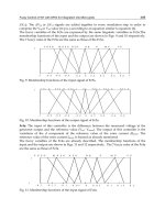
Gas velocity vectors have been shown in figure 6. As this figure represents, the best mixing
of phases happens around caps. Such circulations around valves also have been reported
elsewhere (Lianghua et al., 2008). Existence of eddies enhances mixing and has an important
effect on mass transfer in a distillation column.


Fig. 6. Gas velocity vectors around caps after 6 s.
4.2 Mass transfer on a valve tray
It is assumed that cyclohexane transfers from liquid to the gas phase, and initial mass
fraction of C
7

H
16
in both phases is about 0.15. Concentration is simulated by simultaneously
solving the CFD model and mass-transfer equation. Mass fraction of C
7
H
16
in liquid phase
versus time has been presented in figure 7. As this figure shows, with passing time mass
fraction of n-heptane in liquid increases. In other words, the concentration of the light
component (C
6
H
12
) in the gas phase increases along time (figure 8) and the C
7
H
16
concentration in this phase decreases. In addition, C
6
H
12
concentration in gas phase at higher
layers increases. Figure 9 shows mass frcation of the light component at three different z and
after 6 s. As contours (figure 8 and 9) illustrate, concentrations are not constant over the
entire tray and they change point by point. This concept also has been found by Bjorn et al.
(2002).
Advanced Topics in Mass Transfer

276

Fig. 7. Changes of n-heptane mass fraction in liquid phase with time.


Fig. 8. Mass fraction contours of C
6
H
12
in the gas phase on an x-z plane after (a) 0.25 s, (b) 0.4
s, and (c) 0.6 s.
As mentioned in figure 5, fluid circulation happenes near the tray wall. Therefore, the liquid
residence time distribution in the same zone is longer than that in other zones. With the
Simulation of Hydrodynamics and Mass Transfer
in a Valve Tray Distillation Column Using Computational Fluid Dynamics Approach

277
increase of the liquid residence time distribution, mass transfer between gas and liquid is
more complete than that in other zones. As the liquid layer moves up, the average
concentration of C
6
H
12
in gas phase increases (figure 9) or C
6
H
12
concentration in liquid
phase decreases.
A simulation test with high initial velocities of phases were done, and it was found that
hydrodynamics have a significant effect on mass transfer. Results of the simulation have

been presented in figure 10. Again liquid circulation were observed near the tray wall, and
the maximum velocity can be seen around z=0.009m (figure 10 (b)). At this z, C
6
H
12

concentration is in the maximum value and after that the mass fraction becomes constant
(figure 10 (c)).


Fig. 9. Mass fraction contours of C
6
H
12
in the gas phase after 6 s at (a) z=0.003m; (b) z=0.009
m and (c) z=0.015m.
Advanced Topics in Mass Transfer

278

Fig. 10. Results at high initial velocities of gas and liquid afterr 6s. (a) The geometry;
(b) Liquid velocity versus z and (c) Changes of C
6
H
12
mass fraction with z.
Figure 11 represents snapshots of gas hold-up at z=0. Fluid hold-up was calculated as the
phase volume fraction. Near the tray, gas is dispersed by the continued liquid, and liquid
hold-up decreases as height increases.

Fig. 11. Gas hold-up at z=0 at (a) 1s,(b) 3s, and (c) 6s.
Simulation of Hydrodynamics and Mass Transfer
in a Valve Tray Distillation Column Using Computational Fluid Dynamics Approach

279
5. Conclusion
A three dimensional two phase flow and mass transfer model was developed for simulation
of hydrodynamics behaviour and concentration distribution in a valve tray of a distillation
column. CFD techniques have been used and governing equations simultaneously were
solved by FLUENT software. Eulerian method was applied in order to predict the behaviour
of two phase flow. Clear liquid height for the system of air-water was calculated and results
were compared with experimental data.
System of cyclohexane-n-heptane also were considered and its mass transfer were
investigated. Eddies near the caps have been observed, and it is found that such circulations
enhances mixing and has an important effect on mass transfer in a distillation column.
Results show that the concentration of the light component (C
6
H
12
) in the vapour phase
increases along time and the C
7
H
16
concentration in the vapour phase decreases. In addition,
concentrations are not constant over the entire tray and they change point by point. This
research showed that CFD is a powerful technique in design and analysis of mass transfer in
distillation columns and the presented model can be used for further study about mass
transfer of valve trays.

6. Acknowledgements
The authors thank the National Iranian Oil Refining & Distribution Company (NIORDC)
because of financial support of this research (contract No. 88-1096). Special thanks to Eng.
Mohammad Reza Mirian for his kind cooperation in this work.
7. References
Alizadehdakhel, A.; Rahimi, M. & Abdulaziz Alsairafi, A. (2010). CFD and experimental
studies on the effect of valve weight on performance of a valve tray column.
Comp.
Chem. Eng.
, 34, 1–8.
Bjorn, I.N.; Gren, U. & Svensson, F. (2002). Simulation and experimental study of
intermediate heat exchange in a sieve tray distillation column.
Comp. Chem. Eng.,
26, 499-505.
Buwa, V.V. & Ranade, V.V. (2002). Dynamics of gas-liquid flow in a rectangular bubble
column: Experiments and single/multi-group CFD simulations.
Chem. Eng. Sci., 57,
22, 4715-4736.
C.H. Fischer & G.L. Quarini, 1998. Three-dimensional heterogeneous modelling of
distillation tray hydraulics. Paper presented at the AIChE Annual Meeting, Miami
Beach, FL, 15-19.
Deen, N.G.; Solberg, T. & Hjertager, B.H. (2001). Large eddy simulation of the gas-liquid
flow in a square cross-sectioned bubble column.
Chem. Eng Sci., 56, 6341-6349.
Delnoij, E.; Kuipers, J.A.M. & van Swaaij, W.P.M. (1999). A three-dimensional CFD model
for gas-liquid bubble columns.
Chem. Eng. Sci., 54, 13/14, 2217-2226.
Fluent 6.2 Users Guide (2005). Fluent Inc., Lebanon.
Hirschberg, S.; Wijn, E.F. & Wehrli, M. (2005). Simulating the two phase flow on column
trays.

Chem. Eng. Res. Des., 83, A12, 1410–1424.
Krishna, R.; Van Baten, J.M.; Ellenberger, J.; Higler, A.P. & Taylor, R. (1999). CFD
simulations of sieve tray hydrodynamics.
Chem. Eng. Res. Des., 77, 639–646.
Advanced Topics in Mass Transfer

280
Li, X.G.; Liuc, D.X.; Xua, Sh.M. & Li, H. (2009). CFD simulation of hydrodynamics of valve
tray.
Chem. Engin. Proc., 48, 145–151.
Lianghua, W.; Juejian, C. & Kejian, Y. (2008). Numerical simulation and analysis of gas flow
field in serrated valve column.
Chin. J. of Chem. Eng., 16, 4, 541-546.
Ling Wang, X.; Jiang Liu, C.; Gang Yuan, X. & Yu, K.T. (2004). Computational fluid
dynamics simulation of three-dimensional liquid flow and mass transfer on
distillation column trays.
Ind. Eng. Chem. Res., 43, 2556-2567.
Liu, C.J.; Yuan, X.G.; Yu, K.T. & Zhu, X.J. (2000). A fluid-dynamics model for flow pattern on
a distillation tray.
Chem. Eng. Sci., 55, 12, 2287-2294.
McFarlane, R.C.; Muller, T.D. & Miller, F.G. (1967). Unsteady-state distribution of fluid
composition in two-phase oil reservoirs undergoing gas injection.
Soc. Petrol. Eng.
J.
, 7, 1, 61-74.
Mehta, B.; Chuang, K.T. & Nandakumar, K. (1998). Model for liquid phase flow on sieve
trays.
Chem. Engin. Res. and Des., 76, 843-848.
Rahbar, R.; Rahimi, M.R.; Shahraki, F. & Zivdar, M. (2006). Efficiencies of sieve tray
distillation columns by CFD simulation.

Chem. Eng. Technol., 29, 3, 326-335.
Sanyal, J.; Marchisio, D.L.; Fox, R.O. & Dhanasekharan, K. (2005). On the comparison
between population balance models for CFD simulation of bubble columns.
Ind.
Eng. Chem. Res.
, 44, 14, 5063-5072.
Solari, R.B.; Bell, R.L. (1986).
Fluid flow patterns and velocity distribution on commerical-
scale sieve trays.
AICHE J., 32, 4, 640-649.
Sokolichin, A.; Eigenberger, G.; (1999). Applicability of the standard turbulence model to the
dynamic simulation of bubble columns. Part I. Detailed numerical simulations,
Chem. Eng. Sci., 54, 2273–2284.
Sun, Z.M.; Yu, K.T.; Yuan, X.G.; Liu, C.J. & Sun, Z.M. (2007). A modified model of
computational mass transfer for distillation column.
Chem. Eng. Sci., 62, 1839 – 1850.
Van Baten, J.M. & Krishna, R. (2000). Modelling sieve tray hydraulics using computational
fluid dynamics.
Chem. Eng. J., 77, 3, 143-151.
We, C.; Farouqali, S.M. & Stahl, C.D. (1969).Experimental and numerical simulation of two-
phase flow with interface mass transfer in one and two dimensions.
Soc. Petrol. Eng.
J.
, 9, 3, 323-337.
Wijn, E.F. (1996). The effect of downcomer layout pattern on tray efficiency.
Chem. Eng. J.,
63, 167-180.
Xigang, Y. & Guocong, Y. (2008). Computational mass transfer method for chemical process
simulation.
Chin. J. of Chem. Eng., 16, 4, 497-502.

YOU, X.Y. (2004). Numerical simulation of mass transfer performance of sieve distillation
trays.
Chem. Biochem. Eng. Q., 18, 3, 223–233.
Yu, K.T.; Huang, J. (1980).
Simulation of large tray and tray efficiency. Paper presented at the
AIChE Spring National Meeting
, Philadelphia.
Yu, K.T.; Yuan, X.G.; You, X.Y. & Liu, C.J. (1999). Computational fluid-dynamics and
experimental verification of two-phase two dimensional flow on a sieve column
tray.
Chem. Eng. Res. Des., 77A, 554-558.
Zhang, M.Q. & Yu, K.T. (1994). Simulation of two-dimensional liquid flow on a distillation
tray.
Chin. J. Chem. Eng., 2, 2, 63-71.


14
Modeling Moisture Movement in Rice
Bhagwati Prakash
1
and Zhongli Pan
1,2

1
University of California, Davis,
2
Western Regional Research Center, ARS, USDA
United States
1. Introduction
Rice is one of the leading food crops in the world with total annual production being about

448 million metric tons on milled rice basis in 2008/09 year (USDA, 2010). Rice is found in
marketplace in different forms depending on level of its subsequent processing. Rough rice
(or paddy rice) is the rice that is obtained just after harvest. After removal of its outer husk
(or hull), it becomes brown rice. Brown rice after milling, where the bran layer and embryo
is removed become whiter in color and is called white rice (or milled rice) that is favored
form of human consumption in most countries.
Rough rice is generally harvested at 18-24% moisture contents on wet basis and requires
drying down to 12-14% for safe storage. At commercial scale, drying is carried out by
blowing heated air over grains causing them to lose moisture rapidly. In addition to drying,
moisture movement inside rice kernels occurs when rice is exposed to dry or humid
environments causing desorption or adsorption of moisture, respectively, during any of pre-
harvest or post-harvest stages.
During any of moisture adsorption or desorption processes, the surface of kernel reaches the
equilibrium moisture content in surrounding environmental conditions very rapidly,
however, at center of kernel moisture changes slowly, developing moisture gradients within
the kernel. Higher magnitudes of such moisture gradients are believed to be one of the
major reasons causing fissures or cracks in rice, which result in broken rice on milling.
Milled rice kernels that are three-fourths or more of the unbroken kernel length are called
head rice while the rest are called broken rice (USDA, 1994). Since the full-length grain is
preferred form of rice, broken rice has typically half market value than that of head rice
(Mossman, 1986; Thompson & Mutters, 2006). Therefore, reducing rice fissuring has been an
important goal in rice drying research.
In last five decades, many researchers have pursued mathematical modeling of rice drying
process. Key objective of such model development was to determine the moisture of the
drying rice sample after certain drying period. Development of models also assisted in
understanding the impact of factors affecting drying process such that drying air
temperature and speed of drying air and optimizes them for reducing drying time, without
performing a large number of experiments. Mathematical models were also used to
determine the moisture gradients within the rice kernels that might affect rice fissuring. In
addition to improve drying process, mathematical models can also help in making decisions

on whether rice at particular moisture can be exposed to certain environmental conditions
for certain period of time without significant fissuring.
Advanced Topics in Mass Transfer

284
Among different moisture adsorption and desorption processes, drying has attracted most
attention of researchers. From modeling perspective, there is very little difference between
these processes except the magnitude of moisture movement is very rapid in case of drying.
Drying process would be the main focus in this chapter, however, important information on
other sorption processes will also be described when necessary. Modeling of two types of
drying: convective air drying by heated air and radiative drying by infrared drying will be
mainly covered in this chapter.
The purpose of this chapter is to illustrate different approaches pursued in modeling of
drying processes in rice. Development of both empirical and theoretical models based upon
principles of mass and heat transfer is described in this chapter. Near the end of chapter,
brief discussion on determination of some of the key hygroscopic and thermal properties is
provided. Our goal is to expose the reader to variety of options available in rice drying
modeling literature and assist them to make well-informed choices for successful
development of rice drying models.
2. Mechanism of moisture movement
During most of agricultural products drying, initially moisture is quickly removed, then is
followed by progressively slower drying rates (Allen, 1960). Fig. 1. shows the typical rice
drying curve of rice. It clearly shows that drying rate, which is slope of the drying curve,
becomes smaller with progress of drying. Such drying is referred as falling rate drying.


Fig. 1. Typical drying curve of rough rice
The cause of falling rate drying is inability of internal moisture movement to convey
moisture to the surface at a rate comparable to that of its removal from the surface. Many
theories were proposed to explain mechanism of internal moisture movement in such falling

rate drying behavior. Some of them are: difference in vapor pressure, liquid diffusion,
capillary flow, pore flow, unimolecular layer movement, multimolecular layer movement,
Modeling Moisture Movement in Rice

285
concentration gradient and solubility of the absorbate. Each of these theories explains some
aspects of drying in some materials but no universally applicable theory has been
substantiated by experiments (Allen, 1960). Srikiateden & Roberts (2007) reviewed these
mechanisms as reported in different solid foods and described the mathematical equations
involved in such mechanisms.
Despite the uncertainty about the actual mechanism of moisture movement, most
researchers (Mannapperuma, 1975; Steffe & Singh, 1980a; Aguerre et al., 1982; Lague, 1990;
Sarker et al. 1994; Igathinathane & Chattopadhyay, 1999a; Meeso et al., 2007; Prakash & Pan,
2009) have described moisture movement in rice drying by Fick’s laws of diffusion. Using
such diffusion mechanism, Lu & Siebenmorgen (1992) have modeled moisture movement
during adsorption and desorption processes. Their models predicted average moisture of
the grain reasonably well. However, it should be noted that this alone does not establish
diffusion as the mechanism of moisture movement in rice. A true criterion for the validity of
the mechanism would be accurate prediction of moisture distribution within the grain
(Hougen et al., 1940), which has not been fully considered in rice drying.
3. Mathematical models
Drying of any material normally involves both heat and mass transfer (or moisture transfer).
Pabis & Henderson (1962) measured the center and surface temperature of yellow shelled
maize kernels during heating by free convection in an oven at 71ºC (i.e. 160ºF). They
observed that the surface and center temperatures differed significantly during the first 3 to
4 minutes only and therefore, grains can be considered isothermal during drying process.
Citing this work as their basis, many researchers have assumed grains to be isothermal
during the drying process and neglected heat transfer within the rice kernel. However, in
case of infrared drying, where heating period is very short (typically less than two minutes),
rice kernel cannot be considered isothermal and heat transfer within the rice kernel must be

considered.
Different approaches were taken to mathematically model the moisture changes during the
drying period. Based on the size of sample, these models can be broadly categorized into
three: thin layer (or single layer) drying models, deep bed drying models and single kernel
drying models. Thin layer drying models were mostly empirical or semi-empirical in nature
while most single kernel drying models were based on mechanism of Fickian diffusion.
Deep bed drying models are generally based on thin layer drying models. It is important to
discuss the concept of equilibrium moisture content before we describe development of
different models in detail.
At any fixed environmental conditions, a wet rice sample continues to lose moisture until an
equilibrium state is reached. This moisture content is called equilibrium moisture content
(EMC). In addition to rice variety, this EMC of a rice sample also depends on the
temperature and humidity of ambient air. When a dry rice sample is exposed to humid
environments, it gains moisture content and equilibrates to a value of EMC, which may be
different than the EMC obtained during the moisture desorption. The difference in EMCs
obtained during adsorption and desorption experiments are due to the different condition of
the grains in their approach to equilibrium conditions (Allen, 1960). They cited Simmonds et
al. (1953), who described the discrepancy between the EMC values obtained during
adsorption and desorption to be due to the living nature of grain, which changes its
chemical and physical nature according to environment.
Advanced Topics in Mass Transfer

286
Allen (1960) described another concept of EMC called dynamic EMC that is different than
from the EMC value discussed previously, which they referred as static EMC. They
considered that use of static EMC is inappropriate for drying process, because physical and
chemical changes in the kernel during such process are very fast compared to the conditions
used to determine static EMC. During drying, kernel surface becomes very dry while inner
kernel has higher moisture content creating high moisture gradients. In such conditions,
kernel surface that is exposed to drying air is not representative of the whole grain. This

causes grain moisture to approach a value that is higher than its static EMC during drying.
This moisture content value is called its dynamic EMC. If drying is conducted through a
large range of moisture contents, this approach may reveal existence of more than one value
of dynamic EMCs. They considered dynamic EMCs to be the logical choice to describe
moisture loss during drying process while for gentle moisture movement processes such as
exposure to humid or dry conditions, use of static EMC was more appropriate.
Bakker-Arkema & Hall (1965) dried alfalfa wafers and found that use of static EMC as
boundary equations in second order differential equation of moisture transfer predicted
drying behavior successfully. When static EMC was used, they found the moisture
diffusivity to be almost constant during all but initial stages of drying. On the other hand,
using dynamic EMC resulted in diffusivity value that changed rapidly with moisture
content. Based on this work, they concluded that use of static EMC is more suitable for some
biological products. In rice drying, most of recent works have used static EMCs in their
models. Unless specified, EMC in this chapter refers to static equilibrium moisture content.
3.1 Thin layer drying model
Utilizing the analogy between heat transfer and drying process (Allen, 1960), drying rate of
grains can be expressed as:

e
M
kM M
t
()
∂
∂
=− −
(1)
where, M (kg water/ kg dry solids) is moisture content of grain, t (s) is the period of drying,
M
e

(kg water/ kg dry solids) is the equilibrium moisture content (EMC) of the drying grain
and k (s
-1
) is the drying constant. This equation was found to be convenient, if dynamic EMC
was used for M
e
(Allen, 1960). Integrated form and solution of this equation is given by:

e
k
M
MtClog( )
2.303
−
=− + (2)

kt
e
oe
MM
M
Re
MM
−
−
==
−
(3)
where, C is the integration coefficient, MR is dimensionless moisture ratio, and M
0

(kg
water/kg dry solids) is the initial moisture content of grains. The value of dynamic EMC
used in such equations are determined using trial and error method by plotting, log(M-M
e
)
versus time for different assumed values of M
e
. For the correct value of M
e
, such plot would
be a straight line. The slope of such straight line is used to determine the drying constant k.
Allen (1960) applied this drying equation to thin layer rice drying experimental data and
found that the M
e
and drying constant k, depended upon initial moisture content,
Modeling Moisture Movement in Rice

287
temperature, humidity and quantity of drying air. The rice drying experimental data also
revealed that initial drying period i.e. up to 30 minutes needs different treatment, since it is
dependent upon M
e
and k values, which is different from those used in later drying periods.
However this transition was smooth and knowledge of precise discontinuity was not
required.
In last fifty years, there has been considerable interest among researchers to use empirical or
semi-empirical models, to describe the drying curves during thin-layer grain drying. Some
of these models are described in Table 1.

Reference Model Equation

Allen (1960)
kt
M
Re
−
=
Henderson (1974)
kt kt
M
RAe Be
12
−−
=+

Agrawal & Singh (1977)
n
kt
M
RAe
−
=
Wang (1978)
M
RAtBt
2
1=+ +
Midilli et al. (2002)
n
kt
M

RAe Bt
−
=
+
Table 1. Thin layer drying model equations
In these models, k, A, B, k
1
, k
2
, n are constants dependent upon drying conditions such as
ambient humidity, temperature of drying air and air flow rate through drying column.
Hacihafizoglu et al. (2008) reviewed twelve such models to describe thin layer drying of
rice. The number of parameters in these models varies from one to four. They conducted
drying experiments on long grain rough rice to determine the parameters of these models
and determined the statistical fit of these models to the drying experimental data. In all but
one model, the correlation coefficient was found to be higher than 0.98, which means that all
of these can describe the thin layer drying of rough rice satisfactorily. As expected, model
developed by Midilli et al. (2002) that has four parameters gave the best fit with the
experimental results.
Advantages of such thin layer drying models are in their simplicity and ease of
development. However, parameters in these models depend on specific drying conditions
and therefore must be experimentally determined for each drying condition.
3.2 Deep bed drying models
In deep bed drying, conditions of drying air and grain vary at different depths making it
difficult to use single value of drying constant and equilibrium moisture content, required in
thin-layer drying equations. Two approaches were taken to model such deep bed drying
systems. First approach required determination of mean bed temperature and then, use the
thin layer drying equation with drying constants at that mean temperature. In second
approach, deep drying bed was considered as series of thin layer drying beds, each having
different temperature and therefore, different drying constants.

Allen (1960) conducted experiments to study deep bed drying of maize and rice and used
principle of dimensional analysis, to determine mean bed temperature. Their predicted
drying times in case of rice and maize drying were close to the actual values, the difference
Advanced Topics in Mass Transfer

288
being less than 10% of total drying periods. Nelson (1960) applied similar dimensional
analysis and theory of similitude to study drying in deep bed grain dryers.
Boyce (1965) conducted enthalpy balances to thin layers of barley during drying, accounting
both sensible heat and latent heat of vaporization and conducted layer by layer calculations
to determine temperature of grains at different depths in the deep bed. Despite involving
extensive computation in this approach, it has considerable merit as it uses the
fundamentals principles of heat transfer, compared to empirical approach of Allen (1960).
Detailed description of deep bed drying models was considered beyond the scope of this
chapter. For detailed information on these models and their implementation on computer
reader can refer to works by Bakker-Arkema et al. (1967), Spencer (1969), Henderson &
Henderson (1968) and Parry (1985).
3.3 Single kernel models
In last three decades, Fick’s laws of diffusion have been extensively used to model moisture
movement within the rice kernel in different forms namely white rice, brown rice and rough
rice. In addition to average kernel moisture, such models also describe moisture distribution
within the rice kernels that can be used to estimate moisture gradients and fissuring in rice.
Some studies (Lague, 1990; Yang et al., 2002; Meeso et al., 2007; Prakash & Pan, 2009) have
also considered heat transport within the kernel in their models.
Different rice varieties have their different physical, thermal and hygroscopic properties.
Depending upon the variety of interest, researchers have determined these properties and
developed appropriate models to describe drying. Detailed description of these modeling
efforts is described in the next section.
4. Single kernel models
4.1 Kernel geometry

Rice kernel has an irregular shape. In addition to its shape, structure and thickness of husk
also varies in the kernel (Fig. 2). Developing mathematical model for irregular shapes is
computer power intensive and hence, most of the times rice kernel is approximated to
simpler shapes such as sphere, cylinder, prolate spheroid and ellipsoid. Depending upon
length-width ratio of milled rice, rice varieties are classified into three grain types: long,
medium and short. Length to width ratio for long grain rice is larger than 3.0, medium grain
rice is 2.0 to 2.9 and short grain rice is lower than 2.0 (USDA, 1994). Selecting the shape of
model depends upon geometry of rice variety under study and computational tools
available to solve the model.
Steffe & Singh (1980a) assumed spherical shape to model short grain rice forms. In rough
rice model, they considered endosperm layer to have spherical shape that is surrounded by
spherical shells of bran and husk. Their brown rice model consisted of endosperm and bran
layers while white rice model consisted endosperm only. Assuming spherical shape made
drying a one-dimensional transport process and easy to solve mathematically.
Prediction of moisture gradients accurately demanded more resemblance to the true shape
of kernel. Lu & Siebenmorgen (1992), Sarkar et al. (1994), Igathinathane & Chattopadhyay
(1999a) and Yang et al. (2002) assumed prolate spheroid shape to model medium and long
grain rices while, Ece and Cihan (1993) considered short cylinder shape to model the short
grain rice kernel. Due to their choice of model geometry, these studies have considered
transport processes in two directions.
Modeling Moisture Movement in Rice

289

Fig. 2. Scanning electron micrograph of transverse section of rough rice (Lemont variety)
Use of prolate spheroid shape is suitable when rice kernel cross-section is circular. In case of
medium grain rice variety Californian M206, kernel cross-section is not circular with one
axis about 40% longer than the other. Table 2 shows the three dimensions of this rice variety.
In this case, we have considered an ellipsoid shape with three unequal axes to represent the
kernel. Here, moisture transport within the kernel is three-dimensional phenomenon.

Dimensions (mm) Weight (mg)
Length Width Thickness
Mean 5.78 2.66 1.85 22.3
White Rice
(Std. Dev.) (0.23) (0.11) (0.08) (0.6)
Mean 5.82 2.78 1.97 25.0
Brown Rice
(Std. Dev.) (0.33) (0.09) (0.08) (0.7)
Mean 6.97 3.16 2.19 31.1
Rough Rice

(Std. Dev.) (0.32) (0.19) (0.08) (0.5)
Table 2. Kernel dimensions and weights of medium grain rice variety Californian M206 at
18% moisture on wet basis
Advanced Topics in Mass Transfer

290
Before drying After drying
Fig. 3. X-ray images of two rough rice kernels before and after drying
In rough rice model, the kernel consists of three isotropic regions namely endosperm (or
white rice), bran and husk. In addition to these regions, small air gap is also present between
bran and husk regions in actual rough rice (Fig. 3). Using X-ray imaging, we observed size
of this air gap to increase with progress of drying. In most models, existence of this air layer
is not considered and moisture transfer resistance due to husk represents the equivalent
resistances of this air gap and the husk region. Moisture transfer resistances present in the
rough rice model are shown in Fig. 4.


Boundar

y
la
y
er Endos
p
erm Bran Husk

Fig. 4. Moisture transport resistances in rough rice drying model
It should be noted that size of rice kernel depends on its moisture content. During the
drying process, rice kernels shrink in size. But, for the sake of simplicity, most researchers
have neglected this shrinkage and assumed rice kernel to have same dimensions during the
drying process.
4.2 Transport equations
Single-phase moisture diffusion and heat conduction is commonly used as the mechanism of
moisture transfer and heat transfer, respectively, within the rice kernel. Fick’s law of diffusion
and Fourier’s law of conduction are commonly used to describe these transport processes
during rice drying, respectively. General equations corresponding to these laws are given by:

M
DM
t
()
∂
∂
=∇• ∇
(4)
Modeling Moisture Movement in Rice

291

p
T
ckTQ
t
()
∂
ρ
∂
=
∇• ∇ + (5)
where, M is the moisture content on dry basis (kg water/kg dry matter), t is time (s),
∇
is
divergence operator, D is moisture diffusivity (m
2
/s),
ρ
is density of rice components
(kg/m
3
), c
p
is specific heat (J.kg
-1
.ºC
-1
), T is temperature (ºC), k is thermal conductivity (W.m
-
1
.ºC

-1
) and Q is volumetric heat generation (W/m
3
).
Depending upon the assumed kernel shape, these transport equations can be applied in
spherical, cylindrical or cartesian co-ordinates. Igathinathane & Chattopadhyay (1999a) have
used prolate spheroid co-ordinates.
4.3 Boundary and initial conditions
Two kind of boundary conditions are commonly found in the moisture transport modeling in
the rice drying literature: Dirichlet boundary condition (i.e. instant moisture equilibration of
kernel surface to the ambient environment) and Newmann boundary condition.
Mannappeeruma (1975), Steffe & Singh (1980a), Lu & Siebenmorgen (1992) and Meeso et al.
(2007) considered Dirichlet boundary condition and assumed kernel surface moisture M
s
(kg
water/kg dry matter) to have the same moisture as the equilibrium moisture content M
e
(kg
water/kg dry matter) of rice in the ambient environmental conditions. This can be written as:

se
M
M=
(6)
Sarker et al. (1994) and Yang et al. (2002) equated the outward moving moisture flux to
moisture taken away by convective air and obtained the following Newmann boundary
condition:

ms e
M

DhMM
n
()
∂
∂
−= −
(7)
where, h
m
(m/s) is the surface moisture transfer coefficient and n is the outward normal at
the kernel surface. It should be noted that Eqn. 6 and Eqn. 7 become identical for larger
values of h
m
.
Due to existing uncertainty on mechanism of moisture movement in the rice kernel, some
researchers have assumed evaporation of liquid moisture to occur both at surface and inside
the kernel (Yang et al., 2002) while others have assumed evaporation to occur only at surface
of kernels (Meeso et al., 2007; Prakash & Pan, 2009).
Assuming evaporation to occur only at kernel surface during drying, heat transfer by
convective air to the rice surface can be equated to the conductive heat entering the surface
and change in enthalpy of evaporating moisture. This enthalpy balance represents the heat
transfer boundary condition and can be described by:

av
sa
TVM
khTT
nAt
()
∂ρλ∂

∂∂
−=−−• (8)
where, h (W.m
-2
.ºC
-1
) is the convective heat transfer coefficient, T
s
(ºC) is the temperature of
rice kernel surface, T
a
(ºC) is the temperature of drying air,
λ
(J/kg) is latent heat of
vaporization, V (m
3
) is the volume of the kernel, A (m
2
) is the total surface area of the kernel
and M
av
(kg water/kg dry solids) is average moisture content of kernel at any given time on
dry basis.
Advanced Topics in Mass Transfer

292
At internal boundaries i.e. bran-husk interface and endosperm-bran interface, moisture and
heat fluxes leaving one region is equated to the respective fluxes entering other region. Rice
is considered to have uniform moisture and temperature throughout the kernel before
drying. This is set as the initial conditions in the models.

4.4 Volumetric heat generation
Assuming moisture evaporation to take place both at surface and inside the kernel, the heat
generation due to such evaporating liquid moisture can be expressed as:

M
Q
M
t1
ρλ ∂
∂
=•
+
(9)
where,
λ
(J/kg) is latent heat of vaporization. Here
M
t
∂
∂
must represent the rate of
change of moisture content in liquid form. Determining this rate would require multiphase
modeling that describes moisture in liquid and vapor phases separately. Such multiphase
approach is not pursued in rice modeling yet. When moisture evaporation is assumed to
occur only at kernel surface then there is no such volumetric generation.
Like other radiations, infrared radiation has power to penetrate the surfaces and generate
heat. Heat transfer from infrared radiations to rice kernels can be modeled in two ways:
assuming penetration of heat inside the kernel surface or assuming no heat penetration i.e.
all of radiation heating the surface only.
Heat generated at certain depth below the kernel surface can be modeled as an exponential

decay (Ginzburg, 1969). Datta & Ni (2002) described the heat generation due to infrared
radiations as following:

p
d
d
s
p
P
Qe
d
−
= (10)
where, P
s
is the infrared radiation power at the surface (W/m
2
), d is the depth from the
surface (m), and d
p
is the penetration depth of infrared radiation (m).
Though assuming heat penetration is more fundamental approach, it requires knowledge of
penetration depth that is still to be determined accurately. Some studies (Meeso, 2007;
Prakash & Pan, 2009) have considered penetration depth of of 1-2 mm that was reported for
grains by Ginzberg (1969) and Nindo et al. (1995). If penetration of heat is not assumed, then
there is no heat generation due to infrared radiation. In such case, all radiation heat falling
over the rice surface should be considered in the heat transfer boundary condition, which
can then be rewritten as:

av

sa s
TVM
khTT P
nAt
()
∂ρλ∂
∂∂
−
=−− • −
(11)
4.5 Solution of models
Analytical and numerical solutions have been used to solve the transport equations in rice
drying. Crank (1979) described analytical solution to Fick’s law of diffusion for regular
shapes such as sphere, cylinder and slab for different boundary conditions.

Aguerre et al. (1982) have assumed rough rice kernel as a homogeneous sphere and
considered instant moisture equilibration of kernel surface to the ambient environment.
Modeling Moisture Movement in Rice

293
They have used the following analytical solution to predict average moisture content (M) of
the kernel at any given time:


e
n
e
M
MnDt
MR

MM n R
22
22 2
1
0
61
exp
π
π
∞
=
⎛⎞
−
== −
⎜⎟
−
⎝⎠
∑
(12)
where, M
0
is the initial moisture content, M
e
is the equilibrium moisture content to rice
kernel at ambient drying conditions and R (m) is the equivalent radius of the rice kernel.
Equivalent radius was determined by equating the volume of rice kernel (V, m
3
) to that of
sphere and is given by:

RV
1
3
3
4
π
⎛⎞
=
⎜⎟
⎝⎠
(13)
It should be noted that neglecting third and higher terms of series in Eqn. 12 result in the
thin-layer drying equation reported by Henderson (1974) in Table 1.
Ece & Cihan (1993) assumed rice as a homogeneous short cylinder with Dirichlet boundary
conditions at surface and used following analytical solution to determine average moisture
constant at any given time:

nm
D
e
R
nm
enm
MM R
MR e
MM L
22
2
2
()

222
11
0
81
αβ
αβ
∞∞
−+
==
−
==
−
∑∑
(14)
where, R (m) is radius of cylinder, L (m) is height of cylinder.
α
n
(n=1,2,…) are the roots of
Bessel function of zero order J
0
(x), and
β
m
(m=1,2,…) are defined as:

(
)
m
mR
L

21
2
π
β
−
=
(15)
Aguerre et al. (1982) and Ece & Cihan (1993) did not consider presence of multiple
components such as endosperm, bran and husk inside their models. If these components are
considered in the model, known analytical solutions cannot be used to solve moisture
transport equations. In such cases, numerical methods such as finite difference and finite
element methods are used to solve heat and moisture transport equations.
Steffe & Singh (1980a) and Meeso et al. (2007) used finite difference methods in their one
dimensional spherical shaped rice models. Igathinathane & Chattopadhyay (1999a) have
used finite difference method in prolate spheroid co-ordinate system to model rice drying in
two dimensions. Advantage of the finite difference method lies in its simplicity of
implementation. However, it is not well suited to solve two or three-dimensional problems
and/or problems consisting of material discontinuity. In such problems, finite element
method is more suitable.
Many general-purpose finite element software packages such as Comsol Multiphysics or
pdetool in MATLAB can be used to solve heat and mass transfer equations involved in the
drying model. Lu & Sibenmorgen (1992), Sarker et al. (1994), Yang et al. (2002) and Prakash
& Pan (2009) have used finite element method in their rice models. The representative
meshed model geometry of rough rice in the three-dimensional model is shown in Fig. 5. As
seen in this figure, only one-eighth of the actual rough rice volume was considered in this
model. This was due to the existence of symmetry about the three axes in the rice kernel.