Developments in Heat Transfer Part 11 potx

Its dimensionless form is:

2
**2
()
sCR s s
sf
rss
Hk
CHU
tz
θ
θ
θθ
τρ
∂∂
=− − +
∂∂
(27)


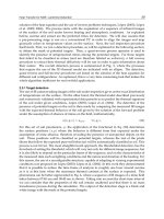
Fig. 9. Comparison of dimensionless energy storage in the ‘washer’, normalized by the ideal
maximum energy change in the ‘washer’, due to different methods of solution
(
(/2)/
washer i s
Bi h d k= =3.0; / 6.0
eq i
Dd

=
;
*2
/[( /2) / ]
is
tt d
α
= ;
c
w = 0.83442)
The parameter cluster of
/( )
sss
kCHU
ρ
is a dimensionless term. If it is sufficiently large, the
axial conduction term in Eq. (27) may not be dropped off. A basic effect of significant axial
heat conduction is that it will destroy the thermocline effect—a temperature gradient with
hot material being on top of cold. This can lower the thermal storage performance in
general. Therefore, to take into account the axial heat conduction effect, a similar correction
via the introduction of another factor to the modified heat transfer coefficient is proposed.
This results in a new modified heat transfer coefficient of:

11
1/
1
p
s
washer c
ss

hh
k
Bi w
CHU
ρ
⎛⎞
⎜⎟
⎛⎞
⎜⎟
=
⎜⎟
+
⎜⎟
⎝⎠
+
⎜⎟
⎝⎠
(28)
For most thermal storage materials, such as rocks, molten salts, concrete, soil, and sands, the
value of
/( )
sss
kCHU
ρ
is very small (in the order of
6
110
−
×
); while other terms in Eq.(27)

are in the order of 1.0. Therefore, the axial heat conduction effect in the thermal storage
material in Eq. (27) is negligible.
5.2.7 Application of the model to the storage system with PCM
For thermal storage with phase-change involved, the PCM can be enclosed in capsules to
form a packed bed as shown in Fig. 2(a), or simply put in a storage tank that has heat
transfer tubes inside as shown in Fig. 2(b). The governing equations discussed above are still

applicable to the heat transfer at locations where either phase change has not yet occurred or
has already been completed. However, at locations undergoing phase change, the energy
equations must account for the melting or solidification process (Halawa & Saman, 2011;
Wu et al., 2011). The key feature in a melting or solidification process is that the temperature
of the material stays constant.
Considering the energy balance for the thermal storage material:

2
()(1)
sm f s
d
hS T T R
dt
ρεπ
Φ
−=−Γ −
(29)
where
Γ is the fusion energy of the material, and
Φ
is the ratio of the liquid mass to the
total mass in the control volume of dz. For melting,
Φ

increases from 0 to 1.0, while for
solidification it decreases from 1.0 to 0.
Considering the invariant of the temperature of the material during a phase change process,
the energy balance equation for HTF is:

2
()
ff
s
mf
ff
TT
hS
TT U
tz
CR
ρεπ
∂
∂
−= +
∂
∂
(30)
Equation (29) and (30) can be reduced to dimensionless equations by introducing the same
group of dimensionless parameters:

**
1
()
ff

mf
r
tz
θ
θ
θθ
τ
∂
∂
−= +
∂
∂
(31)

*
()
CR
mf
r
H
d
dt
ψθ θ
τ
Φ
−−=
(32)
where a new dimensionless parameter
()/
HLs

TTC
ψ
=
−Γ is introduced. Since the phase
change temperature is known, Eqs. (31) and (32) can be solved separately.
5.3 Numerical methods and solution to governing equations
5.3.1 Solution for the case of no phase change
A number of analyses and solutions to the heat transfer governing equations of a working
fluid flowing through a packed-bed have been presented in the past (Schumann, 1929;
Shitzer & Levy, 1983; McMahan, 2006; Beasley, 1984; Zarty & Juddaimi, 1987). As the
pioneering work, Schumann (Schumann, 1929) presented a set of equations governing the
energy conservation of fluid flow through porous media. Schumann’s equations have been
widely adopted in the analysis of thermocline heat storage utilizing solid filler material
inside a tank. His analysis and solutions were for the special case where there is a fixed fluid
temperature at the inlet to the storage system. In most solar thermal storage applications this
may not be the actual situation. To overcome this limitation, Shitzer and Levy (Shitzer &
Levy, 1983) employed Duhamel’s theorem on the basis of Schumann’s solution to consider a
transient inlet fluid temperature to the storage system. The analysis of Schumann, and
Shitzer and Levy, however, still carry with them some limitations. Their method does not
consider a non-uniform initial temperature distribution. For a heat storage system,
particularly in a solar thermal power plant, heat charge and discharge are cycled daily. The
initial temperature field of a heat charge process is dictated by the most recently completed

heat discharge process, and vice versa. Therefore, non-uniform and nonlinear temperature
distribution is typical for both charge and discharge processes. To consider a non-uniform
initial temperature distribution and varying fluid temperature at the inlet in a heat storage
system, numerical methods have been deployed by researchers in the past.
To avoid the long mathematical analysis necessary in analytical solutions, numerical
methods used to solve the Schumann equations were discussed in the literature by
McMahan (McMahan, 2006, 2007), and Pacheco et al. (Pacheco et al., 2002), and

demonstrated in the TRNSYS software developed by Kolb and Hassani (Kolb & Hassani,
2006). Based on the regular finite-difference method, McMahan provided both explicit and
implicit discretized equations for the Schumann equations. Whereas the explicit solution
method had serious stability issues, the implicit solution method encountered an additional
computational overhead, thus requiring a dramatic amount of computation time. The
solution for the complete power plant with thermocline storage provided by the TRNSYS
model in Kolb’s work (Kolb & Hassani, 2006) cites the short time step requirement for the
differential equations of the thermocline as one major source of computer time
consumption. To overcome the problems encountered in the explicit and implicit methods,
McMahan et al. also proposed an infinite-NTU method (McMahan, 2006, 2007). This model
however is limited to the case in which the heat transfer of the fluid compared to the heat
storage in fluid is extremely large.
The present study has approached the governing equations using a different numerical
method (Van Lew et al., 2011). The governing equations have been reduced to
dimensionless forms which allow for a universal application of the solution. The
dimensionless hyperbolic type equations are solved numerically by the method of
characteristics. This numerical method overcomes the numerical difficulties encountered in
McMahan’s work—explicit, implicit, and the restriction on infinite-NTU method (McMahan,
2006, 2007). The current model yields a direct solution to the discretized equations (with no
iterative computation needed) and completely eliminates any computational overhead. A
grid-independent solution is obtained at a small number of nodes. The method of
characteristics and the present numerical solution has proven to be a fast, efficient, and
accurate algorithm for the Schumann equations.
The non-dimensional energy balance equations for the heat transfer fluid and filler material
can be solved numerically along the characteristics (Courant & Hilbert, 1962; Polyanin, 2002;
Ferziger, 1998). Equation (9) can be reduced along the characteristic
**
zt = so that:

)(

1
Dt
D
fr
r
*
f
θθ
τ
θ
−=
(33)
Separating and integrating along the characteristic, the equation becomes:

∫∫
−=
*
fr
r
f
dt)(
1
d
θθ
τ
θ
(34)
Similarly, Eq.(12) for the energy balance for the filler material is reposed along the
characteristic
*

z
=constant so that:

)(
H
dt
d
fr
r
CR
*
r
θθ
τ
θ
−−=
(35)

The solution for Eq. (35) is very similar to that for Eq. (33) but with the additional factor of
CR
H . The term
CR
H is simply a fractional ratio of fluid heat capacitance to filler heat
capacitance. Therefore, the equation for the solution of
r
θ
will react with a dampened speed
when compared to
f
θ

, as the filler material must have the capacity to store the energy
being delivered to it, or vice versa. Finally, separating and integrating along the characteristic
for Eq.(35) results in:

∫∫
−−=
*
fr
r
CR
r
dt)(
H
d
θθ
τ
θ
(36)
There are now two characteristic equations bound to intersections of time and space. A
discretized grid of points, laid over the time-space dimensions will have nodes at these
intersecting points. A diagram of these points in a matrix is shown in Fig. 10. In space, there
are
i = 1, 2, . . . ,M nodes broken up into step sizes of
*
z
Δ
to span all of
*
z
. Similarly, in

time, there are
j = 1, 2, . . . ,N nodes broken up into time-steps of
*
t
Δ
to span all of
*
t .
Looking at a grid of the
ϑ
nodes, a clear picture of the solution can arise. To demonstrate a
calculation of the solution we can look at a specific point in time, along
*
z
where there are
two points,
1,1
ϑ
and
1,2
ϑ
. These two points are the starting points of their respective
characteristic waves described by Eq. (33) and (36). After the time
*
t
Δ
there is a third point
2,2
ϑ
which has been reached by both wave equations. Therefore, Eq. (34) can be integrated

numerically as:

∫∫
−=
2,2
1,1
2,2
1,1
*
fr
r
f
dt)(
1
d
ϑ
ϑ
ϑ
ϑ
θθ
τ
θ
(37)
The numerical integration of the right hand side is performed via the trapezoidal rule and
the solution is:

*
ffrr
r
ff

t
22
1
1,12,21,12,2
1,12,2
Δ
θθθθ
τ
θθ
⎟
⎟
⎠
⎞
⎜
⎜
⎝
⎛
+
−
+
=−
(38)
where
1,1
f
θ
is the value of
f
θ
at

1,1
ϑ
, and
2,2
f
θ
is the value of
f
θ
at
2,2
ϑ
, and similarly so
for
r
θ
.
The integration for Eq. (36) along
*
z
=constant is:

∫∫
−−=
22
12
22
12
,
,

,
,
*
fr
r
CR
r
dt)](
H
[d
ϑ
ϑ
ϑ
ϑ
θθ
τ
θ
(39)
The numerical integration of the right hand side is also performed via the trapezoidal rule
and the solution is:

*
ffrr
r
CR
rr
t
22
H
1,22,21,22,2

1,22,2
Δ
θ
θ
θ
θ
τ
θθ
⎟
⎟
⎠
⎞
⎜
⎜
⎝
⎛
+
−
+
−=−
(40)
Equations (38) and (40) can be reposed as a system of algebraic equations for two
unknowns,
2,2
f
θ
and
2,2
r
θ

, while
f
θ
and
r
θ
at grid points
1,1
ϑ
and
1,2
ϑ
are known.


⎥
⎥
⎥
⎥
⎥
⎦
⎤
⎢
⎢
⎢
⎢
⎢
⎣
⎡
⎟

⎟
⎠
⎞
⎜
⎜
⎝
⎛
−+
⎟
⎟
⎠
⎞
⎜
⎜
⎝
⎛
+
⎟
⎟
⎠
⎞
⎜
⎜
⎝
⎛
−
=
⎥
⎥
⎥

⎥
⎥
⎦
⎤
⎢
⎢
⎢
⎢
⎢
⎣
⎡
⎥
⎥
⎥
⎥
⎦
⎤
⎢
⎢
⎢
⎢
⎣
⎡
+−
−+
r
*
CR
r
r

*
CR
f
r
*
r
r
*
f
r
f
r
*
CR
r
*
CR
r
*
r
*
2
tH
1
2
tH
2
t
2
t

1
2
tH
1
2
tH
2
t
2
t
1
1,21,2
1,11,1
2,2
2,2
τ
Δ
θ
τ
Δ
θ
τ
Δ
θ
τ
Δ
θ
θ
θ
τ

Δ
τ
Δ
τ
Δ
τ
Δ
(41)
Cramer’s rule (Ferziger, 1998) can be applied to obtain the solution efficiently. It is
important to note that all coefficients/terms in Eq.(41) are independent of
*
z ,
*
t ,
f
θ
, and
r
θ
, thus they can be evaluated once for all. Therefore, the numerical computation takes a
minimum of computing time, and is much more efficient than the method applied in
references (McMahan, 2006, 2007).


Fig. 10. Diagram of the solution matrix arising from the method of characteristics
From the grid matrix in Fig.10 it is seen that the temperatures of the filler and fluid at grids
1,i
ϑ
are the initial conditions. The temperatures of the fluid and filler at grid
1,1

ϑ
are the
inlet conditions which vary with time. The inlet temperature for the fluid versus time is
given. The filler temperature (as a function of time) at the inlet can be easily obtained using
Eq.(12), for which the inlet fluid temperature is known. Now, as the conditions at
1,1
ϑ
,
2,1
ϑ
,
and
1,2
ϑ
are known, the temperatures of the rocks and fluid at
2,2
ϑ
will be easily calculated
from Eq.(41).
Extending the above sample calculation to all points in the
ϑ
grid of time and space will
give the entire matrix of solutions in time and space for both the rocks and fluid. While the
march of
*
z
Δ
steps is limited to 1z
*
=

the march of time
*
t
Δ
has no limitation.
The above numerical integrations used the trapezoidal rule; the error of such an
implementation is not straightforwardly analyzed but the formal accuracy is on the order of
)t(O
2*
Δ
for functions (Ferziger, 1998) such as those solved in this study.
5.3.2 Solutions for the case with phase change
For the governing equations of the phase change case, the adopted convention of having the
z-direction coordinate always follow the flow direction is preserved, such that for heat

charging, z=0 is for the top of a tank, and for heat discharging, z=0 is for the bottom of a
tank. The two governing equations (Eq. (31) and Eq.(32)) for the phase change process can
be discretized using finite control volume methodology:

** * ** **
**
() () () ( 1)
()
**
1
()
tt t tt tt
fi fi fi fi
tt
mfi

r
tz
θθθθ
θθ
τ
+Δ +Δ +Δ
−
+Δ
−−
−= +
ΔΔ
(42)

** *
**
()
*
()
tt t
tt
CR i i
mfi
r
H
t
ψθ θ
τ
+Δ
+Δ
Φ

−Φ
−−=
Δ
(43)
From Eq.(42) the fluid temperature
**
()
tt
fi
θ
+
Δ
can be solved, which is then used in Eq. (43) to
solve for the fusion ratio
**
tt
i
+
Δ
Φ .
The procedures for finding the solution of phase change problem are as follows:
1.
Solve the non-phase-change governing equation analytically using Eq.(12) for the phase
change material for the inlet point.
2.
Monitor the temperature at each time step as given by Eq.(12), and see if the
temperature at a time step is greater than the fusion temperature, if yes, the solution for
that and subsequent time steps are to be solved using the phase change equation (Eq.
(43)
3.

For each time step solved using Eq (43), monitor the fusion ratio,
Φ
; when it becomes
larger than 1.0 then the solution for that and subsequent time steps are to be solved
using the non-phase-change governing equation (Eq.(12)) for the remainder of the
required time.
4.
March a spatial step forward and repeat all of the above steps. However, now in part (1)
of this procedure, Eq.(41) must be used to solve the temperatures of both the fluid and
PCM for time steps before phase change starts; and also in part (3) of this procedure
Eq.(41) should be used to solve the temperatures of the fluid and PCM for steps after
the phase change is over. The repetition of parts (1) to (3) of this procedure is to be
continued until all the spatial steps are covered.
6. Results from simulations and experimental tests
6.1 Numerical results for the temperature variation in a packed bed
The first analysis of the storage system was done on a single tank configuration of a chosen
geometry, using a filler and fluid with given thermodynamic properties. The advantage of
having the governing equations reduced to their dimensionless form is that by finding the
values of two dimensionless parameters (
r
τ
and
CR
H ) all the necessary information about
the problem is known. The properties of the fluid and filler rocks, as well as the tank
dimensions, which determined
r
τ
and
CR

H for the example problem, are summarized in
Table 7.
The numerical computation started from a discharge process assuming initial conditions of
an ideally charged tank with the fluid and rocks both having the same high temperature
throughout the entire tank, i.e. 1
fs
θ
θ
=
= . After the heat discharge, the temperature
distribution in the tank is taken as the initial condition of the following charge process. The
discharge and charge time were each set to 4 hours. The fluid mass flow rate was
determined such that an empty (no filler) tank was sure to be filled by the fluid in 4 hours.

With the current configuration, after five discharge and charge cycles the results of all
subsequent discharge processes were identical—likewise for the charge processes. It is
therefore assumed that the solution is then independent of the first-initial condition. The
data presented in the following portions of this section are the results from the cyclic
discharge and charge processes after 5 cycles.

ε

r
τ

CR
H
H R
t
0.25 0.0152 0.3051 14.6 m 7.3 m

Fluid (Therminol
®
VP-1 ) properties:
T
H
=395 °C; T
L
=310 °C;
f
ρ
=753.75 kg/m
3
;
C
f
=2474.5 J/(kg K);
k
f
=0.086W/(m K);
m

=128.74 kg/s;
f
μ
=1.8
4
10 Pa s
−
×
⋅ ;

Filler material (granite rocks) properties:
s
ρ

= 2630 kg/m3;
C
s
=775 J/(kg K); k
s
=2.8 W/(m K); d
r
= 0.04 m;
Table 7. Dimensions and parameters of a thermocline tank (Van Lew et al., 2011)


Fig. 11. Dimensionless fluid temperature profile in the tank for every 0.5 hours
Shown in Fig. 11 are the temperature profiles in the tank during a discharge process, in
which cold fluid enters into the tank from bottom of the tank. The location of
*
0z = is at the
bottom of a tank for a discharge process. The temperature profile evolves as discharging
proceeds, showing the heat wave propagation and the high temperature fluid moving out of

the storage tank. The fluid temperature at the exit (
*
1z
=
) of the tank gradually decreases
after 3 hours of discharge. At the end of the discharge process, the temperature distribution
along the tank is shown in Fig. 12. At this time the fluid and rock temperatures,

f
θ
and
s
θ
respectively (
s
θ
is denoted by
r
θ
when the filler material is rock), in the region with
*
z
below 0.7 are almost zero, which means that the heat in the rocks in this region has been
completely extracted by the passing fluid. In the region from
*
0.7z = to
*
1.0z = the
temperature of the fluid and rock gradually becomes higher, which indicates that some heat
has remained in the tank.


Fig. 12. Dimensionless temperature distribution in the tank after time t
*
= 4 of discharge
(Here
r
θ

is used to denote
s
θ
, as rocks are used as the storage material in the example).


Fig. 13. Dimensionless temperature distribution in the tank after time t
*
= 4 of charge

(Here
r
θ
is used to denote
s
θ
, as rocks are used as the storage material in the example)
A heat charge process exhibits a similar heat wave propagation scenario. The temperature
for the filler and fluid along the flow direction is shown in Fig. 13 after a 4 hour charging
process. During a charge process, fluid flows into the tank from the top, where
*
z is set as
zero. It is seen that for the bottom region (
*
z
from 0.7 to 1.0) the temperatures of the fluid
and rocks decrease significantly. A slight temperature difference between heat transfer fluid
and rocks also exists in this region.

Fig. 14. Dimensionless temperature histories of the exit fluid at z
*
= 1 for charge and
discharge processes
The next plots of interest are the variation of
f
θ
at
*
1z
=
as dimensionless time progresses
for a charging or discharging process. Figure 14 shows the behavior of
f
θ
at the outlet
during both charge and discharge cycles. For the charge cycle,
f
θ
begins to increase when
all of the initially cold fluid has been ejected from the thermocline tank. For the present
thermocline tank, the fluid that first entered the tank at the start of the cycle has moved
completely through the tank at
*
1t
=
, which also indicates that the initially-existing cold
fluid of the tank has been ejected from the tank. Similarly, during the discharge cycle, after
the initially-existing hot fluid in the tank has been ejected, the cold fluid that first entered
the tank from the bottom at the start of the cycle has moved completely through the tank at

*
1t =
. At
*
2.5t =
, or t=2.5 hours, the fluid temperature
f
θ
starts to drop. This is because
the energy from the rock bed has been significantly depleted and incoming cold fluid no
longer can be heated to
f
θ
= 1 by the time it exits the storage tank.
The above numerical results agree with the expected scenario as described in section 4. To
validate the above numerical method, analytical solutions were obtained using a Laplace
Transform method by the current authors (Karaki, et al, 2010), which were only possible for
cases with a constant inlet fluid temperature and a simple initial temperature profile. Results
compared in Fig. 15 are obtained under the same operational conditions—starting from a

fully charged initial state and run for 5 iterations of cyclic discharge and charge processes.
The fluid temperature distribution along the tank (
*
z =0 for bottom of the tank) from numerical
results agrees with the analytical results very well. This comparison essentially proves the
effectiveness and reliability of the numerical method developed in the present study.


Fig. 15. Comparison of numerical and analytical results of the temperature distribution in
the tank after time t

*
= 4 of a discharge (Here
r
θ
is used to denote
s
θ
, as rocks are used as
the storage material in the example)
Based on the results shown in Fig. 15, the temperature distribution along
*
z at the end of a
charge is nonlinear. This distribution will be the initial condition for the next discharge
cycle. Similarly a discharge process will result in a nonlinear temperature distribution,
which will be the initial condition for the next charge. It is evident that the analytical
solutions developed by Schumann (Schumann, 1929) could not handle this type of situation.


Fig. 16. Comparison of dimensionless temperature distributions in the tank after time t
*
= 4
of discharge for different numbers of discretized nodes

Another special comparison was made to demonstrate the efficiency of the method of
characteristics at solving the dimensionless form of the governing equations. Shown in Fig.
16 are the temperature profiles at
*
4t
=
obtained by using different numbers of nodes (20,

100, and 1000) for
*
z . The high level of accuracy of the current numerical method, even with
only 20 nodes, demonstrates the accuracy and stability of the method with minimal
computing time.
6.2 Comparison of modeling results with experimental data from literature
6.2.1 Temperature variations in charge processes
The authors have conducted experimental tests (Karaki at al., 2011). The test conditions for a
given heat charge process are listed in Table 8, which also shows the dimensionless
parameters. As shown in Fig. 17, at the initial time the thermocline tank has a uniform
temperature equal to room temperature. The temperature readings from the thermocouples
at the top of the tank provide the inlet fluid temperatures in a charge process.

Tank Length 0.65(m)
Initial temperature 21.9 (
o
C)
Tank inner diameter 0.241 (m)
High temperature 79.82 (
o
C)
Rock nominal diameter 0.01 (m)
Low temperature 21.9 (
o
C)
Oil flow rate 1.0 (Liter/min.)
Porosity 0.324
Density of rocks 2632.8 kg/m
3
/( / )

cc
tHU
Π
= 7.2511
Charging period t
c
70.08 (min.)
r
τ
0.1262
Rock heat capacity 790 (J/(kg K))
CR
H
0.4068
Time (s) 0 856 1713 2570 3427 4284
Dimensionless time t* 0 1.45 2.9 4.35 5.80 7.25
Table 8. Conditions of a heat charging test (HTF is Xceltherm 600 by Radco Industries)

0
10
20
30
40
50
60
70
80
90
0 1000 2000 3000 4000 5000
Time (second)

Temperature (
o
C)
TC-1
TC-2
TC-3
TC-4
TC-5
TC-6
TC-7
TC-8
TC-9
TC-1 0
TC-1 1
TC-1 2
TC-1 3
TC-1 4

Fig. 17. Temperatures in the center of the tank along the height of 65 cm for a charging
process (Thermocouples were set every 5cm)

0 0.1 0.2 0.3 0.4 0.5 0.6 0.7 0.8 0.9 1
0
0.1
0.2
0.3
0.4
0.5
0.6
0.7

0.8
0.9
1
z
*
θ
f


t
*
=
1.
45
t
*
=
2.
90
t
*
=4
.35
t
*
=
5.80
t
*
=

7.25
z
∗

θ
avg


Fig. 18. The temperature distribution along the height in the tank at different time points
(Solid lines are from simulation results and dashed lines are from experimental tests)
Based on the temperature measurements, the temperature in the tank increases gradually
and at the end of the charging process, the temperatures at all the locations are sufficiently
high. The temperature distribution along the height in the tank at different times is shown in
Fig. 18. Obviously at the end of the charge, the temperature at the top of the tank (at z*=0) is
high. Using the initial temperature distribution and the inlet fluid temperature, together
with the properties listed in Table 8, numerical simulation results were obtained and are
shown in Fig. 18 for the average temperature of the fluid and rocks. The real time and the
dimensionless time are listed in Table 8. The agreement between the experimental data and
the modeling simulation is very satisfactory.
The thermal storage performance test results of a thermocline tank reported in the literature
(Pacheco et al., 2002) was also referenced to validate the current modeling work. The
experimental tests used eutectic molten salt (NaNO
3
-KNO
3
, 50% by 50%) as the heat transfer
fluid and quartzite rocks and silica sands as the filler material. Thermocouples in the test
apparatus were imbedded in the packed-bed. Temperatures in the tank at different height
locations were recorded during a two-hour heat discharge process after the tank was
charged for the same length of time. The storage tank dimensions, packed-bed porosity, and

properties of the fluid and filler material are listed in Table 9.
Using the modeling of section 5, the heat charge followed by heat discharge was simulated.
In Fig. 19, the predicted temperatures at several height locations of the tank at different time
instances during the discharge process were compared to the experimental data reported
(Pacheco et al., 2002). The trend of temperature curves from the modeling prediction and the
experiment is quite consistent. Considering the uncertainties in the experimental test and
the properties of materials considered, the agreement between the experimental data and
the modeling prediction is quite satisfactory. This comparasion firmly validates the current
modeling and its numerical solution method.

ε

r
τ

CR
H
H R
t
0.22 0.0041 0.2733 6.1m 1.5m 2 hr
Molten salt NaNO
3
-KNO
3
properties:
T
H
=396 °C; T
L
=290 °C;

f
ρ
=1733 kg/m
3
;
C
f
=1550 J/(kg K);
k
f
=0.57 W/(m K);
m

=7.0 kg/s;
f
μ
= 0.0021 Pa s⋅ ;
Quartzite rocks/sands mixture properties:
s
ρ

= 2640 kg/m3;
C
s
=1050 J/(kg K); k
s
=2.5 W/(m K); d
r
= 0.015 m;
Table 9. Dimensions and parameters of a thermocline tank for the test in literature (Pacheco

et al., 2002)

Tank Length measured 0.65(m)
Initial temperature 129.0 (
o
C)
Tank inner diameter 0.241 (m)
High temperature 129.0 (
o
C)
Rock nominal diameter 0.01 (m)
Low temperature 56.0 (
o
C)
Oil flow rate 1.96 (Liter/min.)
Porosity 0.324
Density of rocks 2632.8 kg/m
3
/( / )
dd
tHU
Π
= 8.0596
Charging period t
c
39.74 (min)
r
τ
0.1044
Rock heat capacity 790 (J/(kg K))

CR
H
0.4210
Time (s) 0 476.2 952.5 1428.7 1905.0 2381.2
Dimensionless time t* 0 1.61192 3.22384 4.83576 6.44768 8.0596
Table 10. Conditions of a discharge test

0
0.1
0.2
0.3
0.4
0.5
0.6
0.7
0.8
0.9
1
0 0.1 0.2 0.3 0.4 0.5 0.6 0.7 0.8 0.9 1
z*=z/H
θ
avg
t*=0 Modeling
t*=0.767 Modeling
t*=1.534 Modeling
t*=2.300 Modeling
t*=3.067 Modeling
t*=0.0 Test
t*=0.767 Test
t*=1.534 Test

t*=2.300 Test
t*=3.067 Test

Fig. 19. Comparison of modeling predicted results with experimental data from reference
(Pacheco et al., 2002)

6.2.2 Temperature variations in a discharge process
A heat discharge experiment was conducted under the conditions listed in Table 10, which
also includes the dimensionless parameters. Shown in Fig. 20 is the temperature variation
versus time at different locations in the tank along the tank height. The thermocouples at the
top (z*=1.0) of the tank measure the temperature of the discharged fluid. The degradation of
discharged fluid temperature is clearly shown in the figure.

0
20
40
60
80
100
120
140
0 500 1000 1500 2000 2500 3000
Time (second)
Temperature (oC)
TC-1 (bottom-in)
TC-2
TC-3
TC-4
TC-5
TC-6

TC-7
TC-8
TC-9
TC-10
TC-11
TC-12
TC-13
TC-14 (top-out)

Fig. 20. Temperatures in the center of the tank along the height of 65 cm for a discharging
process (Thermocouples were set every 5cm)

0 0.1 0.2 0.3 0.4 0.5 0.6 0.7 0.8 0.9 1
0
0.1
0.2
0.3
0.4
0.5
0.6
0.7
0.8
0.9
1
z
*
θ
f

t
*
=6.44
t
*
=
3.
22
t
*
=1
.6
1
t
*
=
4.
84
t
*
=0.0
t
*
=8.06

θ
avg


Fig. 21. The temperature distribution along the height in the tank at different time points

(Solid lines are from simulation results and dashed lines are from experimental tests)

The temperature distribution along the height in the tank at different times is shown in Fig.
21. At the end of the discharge, the temperature on top of the tank (at z*=1) becomes low,
which means that stored energy has been discharged. Using the measured initial
temperature distribution and the inlet fluid temperature (at z*=1) together with the
properties listed in Table 10, numerical simulation results were obtained and are compared
with the test results in Fig. 21. The real time and the dimensionless time are listed in Table
10. Again, the agreement between the experimental data and the modeling simulation is
satisfactory.
6.3 Correlation of energy delivery effectiveness to dimensionless parameters
Based on the above discussion and the dimensionless governing equations obtained in
section 5.2.3, the energy delivery effectiveness,
η
, is a function of four dimensionless
parameters,
/
cd
ΠΠ,
d
Π
,
r
τ
, and
CR
H . Solutions of the dimensionless governing
equations for energy charge and discharge allow us to develop a database so that a series of
charts and diagrams for
(/, ,, )

cddrCR
fH
ητ
=ΠΠΠ may be prepared for reference by
engineers in the design of thermocline storage tanks. Illustrated in Fig. 22 is a configuration
of a group of database charts for a given
d
Π
, in which multiple graphs, each with a specific
r
τ
, may be provided. In each graph, multiple curves, each with a given H
CR
, for the energy
storage effectiveness
η
versus /
cd
Π
Π are provided. To build a large database, more
graphs in the same configuration can be provided covering a large range of
d
Π
values.

2.0
τ
ri

0.5

η
τ
r1

τ
r2

τ
r3

τ
r4

τ
r5

Π
c
/
Π
d

1.0
0.0
H
CR1

H
CRn

H
CR

A
symptote
0.5
1.0

Fig. 22. Configuration of a group of database charts including multiple graphs of
η
versus
/
cd
ΠΠat a fixed
d
Π

It is easy to understand that under the same mass flow rate and a desired
d
Π
, the energy
delivery effectiveness will increase with the increase of
/
cd
Π
Π
. The asymptote of the
energy delivery effectiveness is due to an ideal thermal storage system, in which
η
can be

exactly 1.0 if the energy charge period is equal to or larger than that of the discharge
(
/1.0
cd
ΠΠ≥
). For any non-ideal thermocline system
η
can only approach 1.0.

Figure 23 shows four charts of
η
versus /
cd
Π
Π at
d
Π
=4.0. Each chart is for a specific
r
τ

with multiple curves for different
CR
H . All the data of energy delivery effectiveness were
obtained based on several cyclic operations of the energy charge and discharge, and the
results are consequently independent of the number of cycles. More charts with wide range
of
d
Π ,
r

τ
, and
CR
H may be developed. However, in actual design practice, the ranges of
d
Π ,
r
τ
, and
CR
H
are not very wide and specific charts can be easily prepared.


(a)
0.01
r
τ
=



(b)
0.04
r
τ
=

(c)
0.1
r
τ
=


(d)
0.2
r
τ
=

Fig. 23. Multiple graphs from modeling results for energy storage effectiveness versus
/
cd
ΠΠat
d
Π =4.0
Observing the above four graphs one can easily draw the following conclusions:
1.
The energy delivery effectiveness never reaches 1.0 if /1.0
cd
ΠΠ< . This proves that
only for an ideal thermocline storage tank can 1.0
η
=
at /1.0
cd
Π

Π= .

2. With the decrease of
r
τ
,
η
will increase. For example, at a ratio of /1.5
cd
Π
Π= and
0.25
CR
H = , the energy delivery effectiveness approaches 1.0 when
r
τ
changes from 0.2
to 0.01. This is because a decrease of
r
τ
is due to an increase in the volume of the
storage tank.
3.
It is understood that a small H
CR
corresponds to the case where ()
s
C
ρ
is relatively large

when compared to ( )
f
C
ρ
, and therefore the energy storage capability is improved, and
η
can approach 1.0 easier. On the other hand, when the void fraction in a packed bed
approaches 1.0, it will make
CR
H →∞, and the thermal storage effectiveness can
approach that of an ideal case. However, in most practical applications, a low void
fraction in a thermocline tank is required for the purpose of using less heat transfer
fluid, and therefore a smaller
CR
H value is practical and preferable.
4.
For cases where
η
could never approach 1.0, even at large
/
cd
Π
Π
values, it is
obviously attributable to the fact that the storage tank is too small, and reselection of a
larger storage tank is needed.
Designers for a thermal storage system often need to calibrate or confirm that a given
storage tank can satisfy an energy delivery requirement. Under such a circumstance, the
dimensions of the storage tank and the power plant operational conditions are known,
which means the values of

r
τ
,
d
Π
, and
CR
H
are essentially given. One can easily check
whether over a range of values of
/
cd
Π
Π the energy delivery effectiveness
η
can
approach 1.0.
7. Procedures of sizing and design of a thermal storage system
The required operational conditions of the power plant dictate the size of the thermocline
storage tank. The relevant operational conditions include: electrical power, thermal efficiency
of the power plant, the extended period of operation based on stored thermal energy, the
required high temperature of the heat transfer fluid from the storage tank, and the low
temperature of the fluid returned from the power plant, the specific choice of heat transfer
fluid and thermal storage material, as well as the packing porosity in a thermocline tank.
The design analysis using the general charts provided in the present study will include the
following steps:
1.
Select a minimum required volume for a thermocline tank using Eqs. (1) and (3).
2.
Choose a radius, R, and the corresponding height, H, from the minimum volume

decided in step (1). Using these dimensions, the parameters—
d
Π
,
r
τ
,
CR
H for a
thermocline tank with filler material, can be evaluated, where
d
Π
is determined based
on the required operational time.
3.
Look up the design charts (such as those in Fig. 23) and see if an energy delivery
effectiveness of 1.0 can be achieved. Often the energy delivery effectiveness will not
approach 1.0 for the first trial design. This is because the first trial uses a minimum
volume. However, with the results from the first trial one can predict the required
height or volume of the tank necessary to decrease
r
τ
and
d
Π
in the same proportion.
A couple of trail iterations may be needed to eventually satisfy the criterion of
η

closing to 1.0.

If the energy delivery effectiveness from step (1) cannot approach 1.0 even if a large
/
cd
ΠΠ
is chosen, one actually has two ways to improve the effectiveness during the second trial.
These are to decrease
CR
H , or decrease both
r
τ
and
d
Π
in the same proportion. However,
CR
H is determined by properties of the fluid and filler material, which has very limited

options, and therefore a decrease of
r
τ
and
d
Π
is more practical. The decrease of
r
τ
can be
done by an increase of the height of a storage tank. This means that to achieve an
effectiveness of 1.0 one has to increase the size of the storage tank. When the height of tank
is increased,

d
Π decreases accordingly since it depends on the height of the tank.
Occasionally, a calibration analysis requires a designer to find a proper time period of
energy charge that can satisfy the needed operation time of a power plant. The known
parameters will be the tank volume,
r
τ
, as well as
CR
H at a required operation period of
d
Π .
The first step of the calibration should be the examination of the criterion given in Eq. (3),
from which a minimum tank volume can be chosen. If the minimum tank volume is
satisfied, the second step of calibration will be to find a proper
/
cd
Π
Π that can make the
energy delivery effectiveness approach 1.0. Graphs including curves at the required
CR
H
and the given
r
τ
and
d
Π
must be looked up. Conclusions can be easily made depending on
whether the energy delivery effectiveness can approach 1.0 for a particular value of

/
cd
ΠΠ.
Two practical examples of thermocline thermal storage tank design are provided to help
industrial designers practice the design procedures proposed in this work. Readers can
easily repeat the design procedures while using their specific material parameters and
operational conditions.
7.1 Design example 1—a system as shown in Fig. 2(a)
A solar thermal power plant has 1.0 MW electrical power output at a thermal efficiency of
20%. The heat transfer fluid used in the solar field is Therminol
®
VP-1. The power plant
requires high and low fluid temperatures of 390 °C and 310 °C, respectively. River rocks are
used as the filler material and the void fraction of packed rocks in the tank is 0.33. The
required time period of energy discharge is 4 hours, the storage tank diameter is chosen to
be 8 m. The rock diameter is 4 cm.
The solution is discussed as follows:
1.
Making use of Eqs. (1) to (3) and the above given details on the power plant, as well as
the properties of Therminol
®
VP-1, we can find a necessary mass flow rate of 25.34
kg/m
3
and an ideal tank height of 9.59 m. The minimum volume of the storage tank can
be determined from Eq. (3). Here, the ideal volume is used in the first trial of the design.
Using Eqs. (19) and (20) we find the modified heat transfer coefficient to be 32.05
W/(m
2
K). With this information, the values of

CR
H ,
d
Π
, and
r
τ
are found to be 0.451,
3.03, and 0.0227, respectively. Given in Fig. 24 is a chart for
d
Π
=3 and
r
τ
=0.0227 at
various values of
CR
H and /
cd
Π
Π . It is seen that on the curve of
CR
H =0.45, there is
no time ratio
/
cd
Π
Π that allows the energy delivery effectiveness to be close to 1.0.
Therefore, the ideal volume chosen will not satisfy the energy storage need.
2.

One option to provide the ability to store and deliver more energy and approach an
effectiveness of 1.0 is to increase the height of the storage tank. When the height is
increased to 12 m, the values of
d
Π
and
r
τ
changed to 2.42 and 0.0181, respectively.
Figure 25 gives the chart for
d
Π
=2.42 and
r
τ
=0.0181. It is seen on the curve of
CR
H =
0.45 that at the time period ratio,
/
cd
Π
Π =1.2, the energy delivery effectiveness
approaches 0.99. This should be an acceptable design.
In this example, compared to an ideal thermal storage tank, the rock-packed-bed
thermocline tank uses about 40.0% of the heat transfer fluid. To avoid the temperature
degradation of the heat transfer fluid in a required discharge time period, a 20% longer
charging time than discharging time is always applied in every charge and discharge cycle.

Fig. 24. Energy delivery effectiveness versus
/
cd
Π
Π at
d
Π
=3 and
r
τ
=0.0227


Fig. 25. Energy delivery effectiveness versus
/
cd
Π
Π at
d
Π
=2.42 and
r
τ
=0.0181
7.2 Design example 2—a system as shown in Fig. 2(b)
For the same solar thermal power plant and operational conditions as in Example 1, the
thermal storage primary material is molten salt with properties of
3
1680 /k
g

m
ρ
= ,
1560 /( )
s
CJkgK=⋅, and 0.61 /( )
s
kWmK
=
⋅ . The heat transfer fluid, Hitec (Bradshaw &
Siegel, 2009), flows in multiple heat transfer tubes, in the same arrangement as shown in Fig.

2(b). The required time period of energy discharge is 4 hours, the storage tank diameter is 8
m. The study will find the storage tank height.
The solution and design procedures are as follows:
3.
Following the same procedure as seen in Example 1, we determine the mass flow rate to
be 40.35 kg/m
3
, and the ideal tank diameter and height to be 8 m and 6.44 m respectively.
It is assumed that we have 8448 steel pipes (with inner diameters of 0.025m) in the
storage tank, and that the heat transfer fluid flows in all of the pipes with an equal flow
rate. The void fraction
ε
is found to be 0.33, and the heat transfer surface area per unit of
length of the tank is found to be
s
S
=1327 m. The modified heat transfer coefficient inside
a pipe for laminar flow heat transfer is used based on the correction using Eqs. (23) to

(25), where the correction coefficient for the washer is
c
w = 3.69894 for the ratio of
/1.74
eq i
Dd= . The minimum volume of the tank is used in the first trial of the design.
The dimensionless values of
CR
H ,
d
Π
, and
r
τ
are 0.522, 3.032, and 0.221, respectively.
Given in Fig. 26 is a chart for
d
Π
=3.032 and
r
τ
=0.221 at various values of
CR
H and
/
cd
ΠΠ
. The figure shows that at an
CR
H

value of 0.50 (close to 0.522) it is impossible
to get an energy efficiency of 1.0 for attempted time ratios of
/
cd
Π
Π up to 2.0.


Fig. 26. Energy delivery effectiveness versus
/
cd
Π
Π at
d
Π
=3.032 and
r
τ
=0.221
To increase the energy delivery efficiency, a new tank height of 2.1 times that of the ideal
volume tank is used. This makes the value of
d
Π
and
r
τ
be 1.444 and 0.105, respectively.
Figure 27 shows the curves for
d
Π

=1.444 and
r
τ
=0.105. It is seen that at an
CR
H value of
0.50 (close to 0.522) and a time period ratio,
/
cd
Π
Π , of 1.2, the energy delivery effectiveness
can reach 0.96.
Note that in the finalized storage tank (with a height of 13.5 m), the volume of heat transfer
fluid takes 69% of the volume of an ideal thermal storage tank (with a height of 6.44 m). The
energy delivery effectiveness reached 0.96 if the charging time period was kept 20% longer
than the required discharge time. Obviously, the weak heat transfer between the HTF and

the primary thermal storage material in Example 2 is responsible for the much larger ratio of
the actual volume compared to the volume of the ideal storage tank. In Example 1 the ratio
of the actual volume of the finalized storage tank is only 1.25 times that of the volume of its
corresponding ideal storage tank. Therefore, it is important that in order to improve the
energy delivery efficiency, the heat transfer between the fluid and thermal storage material
must be improved, for example, by using pipes with fins. Nevertheless, this type of thermal
storage system, as in Example 2, still saves 31% of the heat transfer fluid.


Fig. 27. Energy delivery effectiveness versus
/
cd
Π

Π at
d
Π
=1.444 and
r
τ
=0.105
Thermal energy storage in soil (Nassar et al., 2006), concrete (Zhang et al., 2004; Laing at al.,
2006; Reuss et al., 1997), and in sands (Wyman, 1980) has similar features to that of the
Example 2. When the heat transfer performance (the multiplication of the heat transfer
coefficient and the heat transfer area) between the heat transfer fluid and thermal storage
material is poor, the energy delivery effectiveness can be rather low. If the temperature
degradation of the discharged fluid is a big concern, for example in a power plant, the
thermal storage system in Example 2 may need enhancement of the heat transfer
performance between the heat transfer fluid and thermal storage material.
8. Concluding remarks
Thermal energy storage is very important to the development of concentrated solar thermal
power technologies. Thermal energy storage is also particularly attractive for large capacity
energy storage. It is becoming more and more common for industrial engineers to be
required to size and design thermal storage systems. Therefore, it is necessary to provide a
general analytical tool for the sizing and design of thermal energy storage systems.
The details of the analytical model provided in this book chapter will help researchers and
industrial engineers to understand the behavior of the heat transfer and energy transport
between heat transfer fluid and thermal energy storage material. Two examples for the

practical design of the size of thermal storage systems were provided for readers to practice
the design process concretely. The authors believe that the currently developed charts,
relating the energy storage efficiency to the properties and parameters of a thermal storage
system, are of great potential to help industrial engineers performing sizing calculations for
thermal storage systems. In this regard, the publication of this chapter is a significant and

timely event.
Due to space limitations, this chapter did not provide a large number of the developed
charts for thermal storage system sizing and design. However, the authors are currently
working to provide a handbook including a large number of design charts covering a wide
range of design parameters that industry will need. It is hoped that the handbook will be
available to readers in the near future.
9. Acknowledgement
The authors are grateful for the support provided by the US Department of Energy and the
National Renewable Energy Laboratory, under DOE Award Number DE-FC36-08GO18155,
and the US Solar Thermal Storage LLC. The Support from the Idaho National Laboratory
under award number 00095573 for phase change thermal storage is also gratefully
acknowledged.
10. Nomenclature
f
a The cross section area of a storage tank (m
2
)
Bi Biot number ( /
p
s
Lh k
=
)
C Heat capacity ( /
o
Jk
g
C
⋅
)

d
r
Nominal diameter of a single filler ‘particle’ (rocks) (m)
D Diameter of a storage tank (m)
D
eq
Equivalent diameter (m)
= Enthalpy of fluid at a location along the axis ( /Jkg)
h Heat transfer coefficient (
2
/
o
WmC)
h
p
Modified heat transfer coefficient (
2
/
o
WmC
)
H Length or height of a storage tank (m)
H
CR
A dimensionless parameter
k Thermal conductivity (
/
o
WmC
)

Lp Characteristic length of ‘particles’ for Biot number.
m

Mass flow rate (kg/s)
N Number of tubes for heat transfer fluid in a storage tank
Pr Prandtl number
Q

Thermal energy involved per unit of time (W)
Q Thermal energy involved ( J )
r Average radius of the filler material (rocks) (m)
R Radius of the storage tank (m)
Re Modified Reynolds number for porous media
Ss Surface area of filler material per unit length of the storage tank ( m )
t Time (sec)
T
H
High temperature of fluid from solar field (°C)
T
L
Low temperature of fluid from power plant (°C)

U Fluid velocity in the axial direction in the storage tank (m/s)
V Volume (
3
m
)
z Location of a fluid element along the axis of the tank (m)
Greek symbols
s

α
Thermal diffusivity (=
/( ))
sss
kC
ρ
[m
2
/s]
ε
Porosity of packed bed in a storage tank.
s
η
Thermal storage efficiency.
T
η
Thermal efficiency of a solar power plant.
Γ
Fusion energy of thermal storage material ( /Jkg)
μ
Dynamic viscosity ( Pa s
⋅
)
Π Dimensionless charge or discharge time
r
τ
A dimensionless parameter
ρ Density (
3
/k

g
m )
θ Dimensionless temperature.
Subscript
c Energy charge process
d Energy discharge process
f Thermal fluid
ref A required reference value
r Rocks
s Filler material (rocks), the primary thermal storage material.
z Location along the axis of the tank
Superscript
* Dimensionless values
11. References
Abdoly, M.A., Rapp, D., 1982, Theoretical and experimental studies of stratified thermocline
storage of hot water, Energy Conversion and Management, Vol. 22, No. 3, 1982, pp.
275-285.
Beasley, D.E., and Clark, J.A., 1984, Transient response of a packed bed for thermal energy
storage, International Journal of Heat and Mass Transfer, 27(9), pp. 1659 –1669.
Becker, M., 1980, Comparison of heat transfer fluid for use in solar thermal power stations.
Electric Power Systems Research, 3 (1980) 139-150.
Bradshaw R.W., Siegel N.P., 2009, Development of molten nitrate salt mixtures for
concentrating solar power systems, paper no. 11538, proc. SolarPACES, Berlin,
Germany, 2009.
Bradshaw, A.V., Johnson, A., McLachlan, N.H., Chiu, Y-T., 1970, Heat transfer between air
and nitrogen and packed beds of non-reacting solids, Trans. Instn Chem. Engrs,
Vol. 48, 1970, pp. T77-T84.
Brosseau, D., Kelton, J.W., Ray, D., Edgar, M., Chisman, K., and Emms, B., 2005, Testing of
thermocline filler materials and molten-salt heat transfer fluids for thermal energy
storage systems in parabolic trough power plants, Journal of Solar Energy

Engineering, 127(1), pp. 109–116.