Advanced Trends in Wireless Communications Part 8 ppt

−60 −40 −20 0 20
−5
−4
−3
−2
−1
0
Shift Percentage
Normalized peak power (dB)
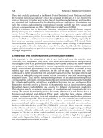
Fig. 9. Received signal peak power with left and right shifts normalized to the peak with no
shift
Fig. 9 shows the peak power of the received signal peak for the shifted signals normalized
to the received peak with no shift. The shift percentage corresponds to the percentage of
the total length of the transmitted signal. A set of 243 measured CIRs are used for the
simulation. Experimental setup and the measurement procedure are explained in Section
4.4. The loss of the received peak power for transmitted signals corresponding to individual
CIRs is represented by the dots and the dashed line is the mean of power loss. To calculate
the maximum number of simultaneous users that a system can support, we must take the
decision in accordance to the threshold (say 3 dB) which can vary for different applications.
Fora3dB threshold, our system can support a shift percentage of 0.70L taps for left shift and
0.25L taps for right shift (see Fig. 9). Thus, the number of users with the proposed scheme can
be written as:
N
mod.TR
u
= 
0.95 × L
δ
 = 
0.95 ×T

si g
ΔTR
 (15)
where
. denotes the floor operator, L is the total number of taps in the transmitted signal, δ is
the shift percentage between two simultaneous users, T
si g
is the channel length in s and ΔTR
is shift separation between two users in s. For the same threshold, the previously proposed
scheme in Nguyen et al. (2006) can only support a shift of 0.75L which is contrary to their
claim of 100% shift (as power loss with circular shift operation was not considered by the
authors). The power loss for left shift is lesser than the power loss for the right shift as the
energy contained in the shifted parts of the right shift is greater than the energy contained in
the shifted parts of the left shift. Although a combination of right and left shifts can be used
for the communication, for the sake of simplicity we have only used a left shift. In the rest of
the paper unless otherwise mentioned, a shift is meant to be a left shift.
The power spectral density (PSD) of the transmitted signal of a TR communication system
takes into account the effects of the antennas and the propagation channel including the path
loss. In contrast to the pulse signal, the spectrum of a TR signal has a descending shape with
increasing the frequency because the higher frequency components experience a greater path
loss as compared to the lower frequency components in the spectrum. Fig. 10 shows the PSD
plots of the transmitted signal with simple TR and modified TR schemes where a left shift
of 0.20N taps is carried out for both modified TR scheme. The plots of both schemes have a
descending shape. Maximum spectral power is experienced at the same frequency. Therefore,
235
Time Reversal Technique for Ultra Wide-band and MIMO Communication Systems
0 2 4 6
−50
−40
−30

−20
−10
0
10
20
Frequency (GHz)
PSD (dBm/MHz)


simple TR
modified TR
Fig. 10. PSD of transmitted signal with simple TR and modified TR schemes
both the signals must be attenuated with the same factor in order to respect the UWB spectral
mask proposed by FCC. Frequency selectivity of the transmitted signals is similar for the two
schemes. In short, the both schemes have resembling spectral properties.
4.4 Experimental setup and simulation results
Experiments are performed in a typical indoor environment. The environment is an office
space of 14 m
× 8 m in the IETR
1
laboratory. The frequency response of the channel in the
frequency range of 0.7-6 GHz is measured using vector network analyzer (VNA) with a
frequency resolution of 3.3 MHz and two wide band conical mono-pole antennas (CMA)
in non line of sight (NLOS) configuration. The height of the transmitter antenna and the
receiver antenna is 1.5 m from the floor. The receiver antenna is moved over a rectangular
surface (65 cm
× 40 cm) with a precise positioner system. The frequency responses between
the transmitting antenna and receiving virtual array are measured. The time domain CIRs
are computed using the inverse fast Fourier transform (IFFT) of the measured frequency
responses.

4.5 BER performance
In the proposed transmission scheme, one user is separated with the other by a shift of a fixed
number of taps. This separation is named as δ, which is a percentage of total number of taps
in the transmitted signal. Signal for User 1 is transmitted without any shift. As discussed in
Section 4.2, that interference between users is greatly reduced with the proposed modulation
scheme. To study the impact of the reduced interference, we evaluate the BER performance
with the proposed scheme using left shift for 5, 10 and 15 simultaneous user for δ
= 0.05 L.
From the measured CIRs, we generate almost 35
×(35 − N
u
−1) combinations for simulating
different number of simultaneous users (N
u
). For every combination of simultaneous users,
10000 symbols are transmitted which makes it sufficient for statistical analysis. The measured
CIR is truncated for 90% energy contained in the CIR. Thus, the transmitted symbol has a
length of 55 ns and a per user bit rate of 18 Mbps. Perfect synchronization and no ISI effects
are assumed. Signal to noise ratio (SNR) is varied by varying the noise variance, as:
SNR
= P
j
/σ
2
noise
(16)
1
Institute of Electronics and Telecommunications of Rennes
236
Advanced Trends in Wireless Communications

10 15 20 25 30
10
−4
10
−3
10
−2
10
−1
10
0
SNR (dB)
BER


5 Users
10 Users
15 Users
(a) Simple-TR
10 15 20 25 30
10
−4
10
−3
10
−2
10
−1
10
0

SNR (dB)
BER


5 Users
10 Users
15 Users
(b) TR with circular shift
10 15 20 25 30
10
−4
10
−3
10
−2
10
−1
10
0
SNR (dB)
BER


5 Users
10 Users
15 Users
(c) Modified-TR scheme
10 15 20 25 30
10
−4

10
−3
10
−2
10
−1
10
0
SNR (dB)
BER


simple TR
TR wcs
Modified TR
(d) All three schemes
Fig. 11. BER performance with 5, 10, and 20 simultaneous users with a) simple TR, b) TR
with circular shift, c) modified TR scheme, d) 15 simultaneous users with all three schemes
for δ
= 0.05 L taps
237
Time Reversal Technique for Ultra Wide-band and MIMO Communication Systems
where P
j
is the power of the received signal at its peak and σ
2
noise
is the noise variance. Bipolar
pulse amplitude modulation (BPAM) is used for these simulations. The received signal y
j

(t)
is sampled at its peak and is detected based on ideal threshold detection, given as:
Detected bit
=

1ify
j
(t
peak
) ≥ 0
0ify
j
(t
peak
) < 0
(17)
Fig. 11a-c shows the BER performance of the simple TR, TR with circular shift operation
and the modified TR scheme for 5, 10 and 15 simultaneous users. The modified TR scheme
outperforms the other two schemes specially for higher number of simultaneous users (10,
15). For instance for 10 simultaneous users, the modified TR scheme results in a 1.4 dB better
performance than the TR with circular shift for a BER of 10
−4
. The simple TR scheme has
already reached a plateau. To perform an analysis in the presence of extreme multi user
interference, BER performance is studied for 15 simultaneous users. Fig. 11d compares the
performance of the three schemes for 15 simultaneous users. The modified TR scheme gives
significantly better performance than the other two schemes. The improvement is in the order
of 4.5 dB or more.
If a system has a large number of users, the users experiencing higher shift percentages will
give poorer performance than the users experiencing lower shift percentages. To have a

consistent system, we propose to rotate the shift percentages for different users so that no
user is subjected to permanent high shift percentage.
5. Conclusion
In this chapter, TR validation with multiple antenna configuration, followed by the parametric
analysis of the TR scheme, is performed by using time domain instruments (AWG and
DSO). Different TR properties such as normalized peak power (NPP), focusing gain (FG),
signal to side-lobe ratio (SSR), increased average power (IAP) and RMS delay spread
are compared for different muli-antenna configurations. It has been found that with
multi-antenna configurations, a significantly better TR peak performance is achieved with
all other properties remain comparable to the SISO-TR scheme.
In the second part of the chapter, a modified transmission scheme for a multi user
time-reversal system is proposed. With the help of mathematical derivations, it is shown
that the interference in the modified TR scheme is reduced compared to simple TR scheme.
Limitations of the proposed scheme are studied and an expression for maximum number of
simultaneous users is proposed. It is shown that the modified TR scheme outperforms simple
TR and TR with circular shift scheme specially at higher number of simultaneous users. For
instance for 15 simultaneous users, the modified TR scheme improves the performance in the
order of 4.5 dB or more for a constant BER.
All these results suggest that the TR UWB, combined with MIMO techniques, is a promising
and attractive transmission approach for future wireless local and personal area networks
(WLAN & WPAN).
238
Advanced Trends in Wireless Communications
6. Acknowledgment
This work was partially supported by ANR Project MIRTEC and French Ministry of
Research.This work is a part of ANR MIRTEC and IGCYC projects, financially supported by
French Ministry of Research and UEB.
7. References
Akogun, A. E., Qiu, R. C. & Guo, N. (2005). Demonstrating time reversal in ultra-wideband
communications using time domain measurements, International Instrumentation

Symposium.
Edelmann, G., Akal, T., Hodgkiss, W., Kim, S., Kuperman, W. & Song, H. C. (2002). An
initial demonstration of underwater acoustic communication using time reversal,
IEEE Journal of Oceanic Engineering 27(3): 602–609.
Fink, M. (1992). Time reversal of ultrasonic fields-part i: Basic principles, IEEE Transactions on
Ultrasonics, Ferroelectrics and Frequency Control 39(5): 555–566.
Fink, M. & et. al. (2000). Time-reversed acoustics, Rep. Progr. Phys 63: 1988–1955.
Guguen, P. & El Zein, G. (2004). Les techniques multi-antennes pour les réseaux sans fil, Hermes
Science Publishers.
Khaleghi, A. & El Zein, G. (2007). Signal frequency and bandwidth effects on the performance
of UWB time-reversal technique, Antennas and Propagation Conference, 2007. LAPC
2007, Loughborough, pp. 97–100.
Khaleghi, A., El Zein, G. & Naqvi, I. (2007). Demonstration of time-reversal in
indoor ultra-wideband communication: Time domain measurement, International
Symposium on Wireless Communication Systems, ISWCS 2007, pp. 465–468.
Kyritsi, P., Eggers, P. & Oprea, A. (2004). MISO time reversal and time compression, Proc.
URSI International Symposium on Electromagnetic Theory.
Kyritsi, P., Papanicolaou, G., Eggers, P. & Oprea, A. (2004). MISO time reversal and
delay-spread compression for FWA channels at 5 ghz, IEEE Antennas and Wireless
Propagation Letters 3: 96–99.
Lerosey, G., De Rosny, J., Tourin, A., Derode, A. & Fink, M. (2006). Time reversal of wideband
microwaves, Appl. Phys. Lett. 15: 154101.
Mo, S. S., Guo, N., Zhang, J. Q. & Qiu, R. C. (2007). UWB MISO time reversal with energy
detector receiver over ISI channels, IEEE Consumer Communications and Networking
Conference, CCNC2007, pp. 629–633.
Naqvi, I. & El Zein, G. (2008). Time domain measurements for a time reversal SIMO system
in reverberation chamber and in an indoor environment, Digest of Papers, IEEE
International Conference on Ultra-Wideband, ICUWB 2008, Vol. 2, pp. 211–214.
Naqvi, I. H. & El Zein, G. (2009). Time reversal UWB system: SISO, SIMO, MISO and MIMO
comparison with time domain experiments, Journées Scientifiques CNFRS-URSI

“Propagation et Télédétection”.
Naqvi, I. H. & El Zein, G. (2010). Retournement temporel en ULB: étude comparative
par mesures pour des configurations multi-antennes, Revue de l’Electricité et de
l’Electronique (REE). Dossier: Propagation et Télédétection (2): 66–72.
Naqvi, I., Khaleghi, A. & El Zein, G. (2007). Performance enhancement of multiuser
time reversal UWB communication system, International Symposium on Wireless
Communication Systems, ISWCS 2007, pp. 567–571.
239
Time Reversal Technique for Ultra Wide-band and MIMO Communication Systems
Naqvi, I., Khaleghi, A. & El Zein, G. (2009). Multiuser time reversal uwb communication
system: A modified transmission approach, IEEE International Symposium On
Personal, Indoor and Mobile Radio Communications (PIMRC ’09).
Nguyen, H., Andersen, J. & Pedersen, G. (2005). The potential use of time reversal techniques
in multiple element antenna systems, IEEE Communications Letters 9(1): 40–42.
Nguyen, H. T., Kovacs, I. & Eggers, P. (2006). A time reversal transmission approach
for multiuser UWB communications, IEEE Transactions on Antennas and Propagation
54(11): 3216–3224.
Oestges, C., Hansen, J., Emami, S. M., Kim, A. D., Papanicolaou, G. & Paulraj, A. J. (2004).
Time reversal techniques for broadband wireless communication systems, European
Microwave Conference (Workshop).
Qiu, R., Zhou, C., Guo, N. & Zhang, J. (2006). Time reversal with MISO for ultrawideband
communications: Experimental results, IEEE Antennas and Wireless Propagation Letters
5(1): 269–273.
240
Advanced Trends in Wireless Communications
Part 5
Vehicular Systems

Robert Nagel and Stefan Morscher
Institute of Communication Networks, Technische Universität München

Germany
1. Introduction
As mobile ad-hoc networks gain momentum and are actively being deployed, providing users
and customers with ubiquitous connectivity and novel applications, some challenges implied
especially by the mobility of users have not yet been solved. Generally, it can be stated
that modern applications impose higher requirements on the underlying communication
solutions: more bandwidth, less packet loss, less delay and more reliability of services in
terms of availability. These performance metrics are commonly termed Quality of Service (QoS).
Due to the variability of node locations in mobile networks, the experienced QoS is highly
time-variant. We have discussed in Nagel (2010a) that the level of attained QoS ultimately
results from a proper combination of connectivity, i.e., the communication relations in a
network, the chosen (and usually invariant) medium access (MAC) protocol and the traffic
that is injected into the network at the nodes. If a certain level QoS is desired in a mobile
wireless network, at least one of these three properties has to be actively controlled.
We have demonstrated that through controlling the amount of traffic that is injected by the
nodes, effective distributed mechanisms can be employed that are, given minimal information
about nodes’ connectivity, able to provide (and even guarantee) a certain level of QoS. These
mechanisms, however, are based on the current connectivity of the network and are effective
only at present time. Should an application require a certain amount of QoS over a larger
period of time, additional provisions become necessary. Although it is possible to control
connectivity in certain boundaries (for instance through power control or adaptive antennas)
and at a certain cost, the fundamental physical causes of connectivity themselves (location,
mobility, and wireless channel state) cannot be influenced by the application as they are
dictated by the user’s behavior and the environment. It is, however, possible to anticipate
a network’s future connectivity – at least for a certain time horizon – and to compute the
resulting future QoS. Upon this information, applications, services, and routing protocols
could be parameterized accordingly: as an example, if the future QoS of a connection using
a certain route is predicted to fall below a necessary level due to a link break, the expected
remaining time until the link actually breaks could be used to proactively find and set up a
backup route that uses other, potentially more stable links. Also, if a connection was to be

set up for a limited time, it may be very helpful to assess if the required QoS can actually be
provided by the network for the desired duration before the connection is actually established.
While other work mainly uses mobility prediction in cellular scenarios to estimate hand-over
times, or to support ad-hoc routing in random-mobility ad hoc scenarios, this chapter

Connectivity Prediction in Mobile Vehicular
Environments Backed By Digital Maps
13
focuses on connectivity prediction in the special case of vehicular networks. Networked
vehicular nodes can be assumed to adhere to certain rules that constitute drivers’ basic
behavior: they move along roads and try to avoid collisions with obstacles, such as buildings
and other cars. Founded on the vehicular scenario constraint, we present an algorithm
that predicts the location of vehicles based on their current state (position and velocity)
and information from digital street maps obtained through the Open Street Map (OSM)
project. A filter-based, self-adaptive velocity prediction algorithm is used to model the
user-inflicted velocity changes. Using their current positions and the predicted velocities,
possible future positions of cars on the street grid and their respective probabilities can be
determined. Although the main focus of this chapter is on mobility prediction, we discuss an
effective channel parameter estimation technique and propose to predict the network’s future
connectivity using an adaptive channel model.
It should be noted that the proposed position prediction mechanism does not completely
exhaust all opportunities provided by the vehicular scenario. For instance, we assume that
vehicles have no information about other vehicles’ missions, i.e., the planned route through
the road grid. Furthermore, we make no assumptions about other vehicles’ capabilities (in
terms of maximum acceleration and deceleration, yaw rate, etc.). Also, we do not consider
environmental properties, such as weather, street and traffic conditions, etc. We will, however,
point out and discuss the potential spots where these additional informations could be
exploited to further augment the proposed algorithm.
In the following Section, we present an overview of current work. Subsequently, in Section 3
we formulate the problem mathematically and in Section 4, we describe our algorithm that

predicts the future positions of vehicles according to their actual state and a complemental
digital road map. In Section 5, we will discuss why the channel model presented in Equation 1
is not sufficient under all conditions and present methods that can adapt to the environment.
In Section 6, we discuss some simulation results. Section 7 summarizes this chapter and gives
an outlook on further work.
2. Related work
One possible way of predicting a network’s future connectivity is to use a model that reflects
the individual mobility properties of a node. Given the knowledge of the initial position
velocity of a node, a future position could be projected by multiplying the velocity vector with
the desired time interval. Obviously, this approach does not account for changes in the length
and/or direction of the velocity vector. Several more sophisticated approaches have been
suggested and today, mobility prediction has become a common research topic in wireless
networks.
Due to the distinct characteristics of vehicular ad-hoc networks, especially the high speeds and
restricted degree of freedom in the movement of vehicles, most of the work on prediction for
ad hoc networks is too general and thus inappropriate for vehicular networks. Nevertheless,
some approaches are discussed here because they give an overview of mobility prediction in
general. Material specific to mobility prediction in vehicular networks is very rare and the
topic is often neglected in works on vehicular ad hoc networks.
Kaaniche & Kamoun (2010) presents an approach for mobility prediction using neural
networks. Although it is not specifically designed for vehicular networks it should perform
better than other general approaches as it is independent of the underlying mobility model.
A trajectory is calculated for multiple steps in the future using several past positions in quite
a similar manner as the adapting FIR filter for velocity prediction presented in this work.
244
Advanced Trends in Wireless Communications
However, the approach does not use any map material and hence the predicted positions may
lie far off the road and may thus be unrealistic. The approach using neural networks could be
used for velocity prediction in the constellation presented in this works to substitute the FIR
filter, however it is expected to perform in a very similar manner and the FIR filter seems less

complex to implement.
A similar approach for mobility prediction using spatial contextual maps and
Dempster-Shafer’s theory for decision making is formulated in Samaan & Karmouch
(2005). A framework is presented that allows prediction of the users mobility trajectory based
on various bits of contextual information from e.g. user profile and map data. The approach
is motivated by the fact that contextual information is becoming more common for adapting
services towards the users needs and it uses the additional information in order to predict the
users mobility. The concept seems feasible for e.g. cell phone users traveling on foot but does
not seem appropriate for vehicular networks as the only contextual information possibly
available and relevant to the future mobility is the chosen route to the destination. A complex
theory to combine evidence into a prediction is not necessary in this case.
Huang et al. (2008) suggests a prediction algorithm based on fuzzy logic that aims at the
prediction of a possible link break or a congested link which then triggers the construction
of an alternate route. Similar to our algorithm, the prediction of a link break is based on the
prediction of the future vehicle speed, the basis on which the predicted distance to the vehicle
can be determined. This requires the generation of a fuzzy rule base that is then dynamically
trained using Particle Swarm optimization (which in our approach is done using the adaptive
filter for speed prediction). The authors use similar ideas in terms of the speed prediction
but implements a fundamentally different concept. Furthermore, it is focussed on route break
prediction and hence the performance of the isolated velocity prediction compared to our
algorithm cannot be easily evaluated.
In Boukerche et al. (2009), the authors present some general thoughts on mobility prediction
in vehicular networks and propose a simple prediction algorithm based on movement vectors
in order to reduce the frequency of location beacons without introducing a higher mean
error in respect to the positions used for routing packets. In Rezende et al. (2009), the same
authors introduce the Network Neighbor Prediction protocol (NNP) that uses the results from
their prior works to predict new routes that are going to be available in the near future
and to calculate the lifetime of those routes that are currently in use. These works show in
their simulation results that mobility prediction is a useful and necessary aspect in vehicular
networks and should be researched in greater detail than it currently is.

Another approach, although developed in the context of a different problem, is described
by Althoff et al. (2010). The authors compute the set of points that could be reached by vehicles
within the prediction times, given the capabilities (minimum and maximum acceleration, yaw
rate, etc). of the considered vehicles. The approach is computationally complex and requires
a lot of contextual information.
Using the predicted position it should also be possible to predict the future connectivity to a
certain extent using an appropriate channel model. In the context of vehicle-to-vehicle (V2V)
communications, there is not yet a widely accepted channel model Paier et al. (2009). A
common approach for characterizing a channel is to work out a theoretical channel model
and then validate it against some appropriate measurements. Channel models are usually
classified into stochastic and deterministic channel models, where deterministic channel
models use ray tracing and similar techniques based on topological information about the
environment in order to solve the the multi-path components (MPC) and derive a precise
245
Connectivity Prediction in Mobile Vehicular Environments Backed By Digital Maps
channel characterization for a specific realization. Stochastic channel models, on the contrary,
try to depict the statistics of the propagation channel in a more general sense that is not so
much focussed on a particular situation. An intermittent approach is taken by geometry based
channel models (as presented in Cheng et al. (2009)) that do use ray tracing; however, instead
of using realistic modeling the calculations are based upon randomly placed objects.
In order to characterize a channel a number of parameters are used:
• The path loss exponent (PLE) α characterizes the average attenuation of the received signal.
• Large scale fading on the one hand refers to slow variations of received power due to
shadowing by obstructing objects.
• Small scale fading on the other hand is caused by interference of different MPCs that
result in fast fluctuations of the received power. Because these fluctuations are very
hard to describe deterministically, they are usually described by means of statistics - most
commonly by a Rayleigh distribution.
• In order to determine how much power is carried by the respective MPCs a power delay
profile (PDP) is used. The spreading of the received pulse in the time division - often

referred to as the channels delay dispersion - is best described in a statistical way by the
root mean squared delay spread.
• Because MPCs travel on different paths they experience different Doppler shifts. The root
mean square Doppler spread describes the resulting spectrum widening of the received
pulse and thus the frequency dispersion.
A large amount of research has been dedicated to the wireless channel in cellular networks.
However, looking at the specifics of a vehicular channel, especially in the V2V case it soon
becomes clear that its characteristics differ significantly from those of a cellular channel.
On the one hand, antennas of both sender and receiver are mounted close to the ground
in V2V communications, where with cellular systems usually one of them is mounted high
above. This tremendously influences the propagation path of the signals and thus the channel
characteristics in terms of diffraction and reflection. On the other hand, communications
between vehicles commonly use the 5.9 GHz band which behaves significantly different than
the 700-2100 MHz signals used in cellular systems in terms of attenuation and diffraction.
Most importantly though, sender and receiver are moving at relatively high speeds in V2V
scenarios, which invalidates the assumption of stationarity of the channel characteristics that
is commonplace in channel models of cellular systems. That refers not only to a changing
impulse response but also to a change of its statistical properties (fading distribution, PDP
and Doppler spectrum) Molisch et al. (2009). According to Maurer et al. (2004), Doppler shift
and Doppler spread characterize the time-variant behavior of the V2V channel mostly due to
movement of the communicating vehicles and the adjacent vehicles.
This section highlights and discusses some of the works into vehicular channel modeling in
the context of connectivity prediction - a topic that has not yet received much attention in
literature. In Matolak et al. (2006), the authors describe a statistical V2V channel model that
is restricted to small scale fading. It uses a tapped delay line model, each tap representing
a multi path components received with a certain delay. Each tap has an on/off switching
process modeled by a first order Markov chain allowing for persistence parameterization. In
general, taps with longer delays have less probability of being on due to their lower energy.
Tap amplitudes are modeled using the Weibull distribution where different parameters are
proposed for different taps, based on some measurements. The authors differentiate between

246
Advanced Trends in Wireless Communications
different scenarios, in some of which the Weibull parameters are “worse than Rayleigh” (β <
2), a phenomenon that is often called severe fading.
Maurer et al. present a geometry based IVC channel model in Maurer et al. (2004). They
first try to model the dynamic road traffic and the environment adjacent to the road and
then try to evaluate multi-path wave propagation through means of ray tracing. The road
traffic model is based on the so called Wiedemann model and uses results from the authors
previous works. As it seems very difficult to obtain real data with the necessary level
of detail and the coverage, a stochastic model is utilized in order to place objects in the
surroundings of the road. Different morphographic classes are defined for urban, suburban
and highway scenarios that are assigned specific probabilities for different types of objects
(trees, buildings, cars, bridges, traffic signs, etc.). Multi-path components are represented
by rays, each of which can experience several propagation phenomena like diffraction or
reflection. By calculating consecutive snapshots, a time-series of channel impulse responses
can be obtained that classifies the channel for the current surrounding. The authors present
measurements that validate the channel model with a standard deviation of less than 3 dB in
both line-of-sight (LOS) and non-line-of-sight (NLOS) scenarios.
Paier et al. (2009) presents some measurements of V2V propagation in suburban driving
conditions using GPS receivers. The authors on the one hand derive both a single slope and
a dual slope path loss model from their results where the better dual slope model achieves
deviations between 2.6 and 5.6 dB compared to the measured path loss. However, they find
that received power is significantly less if no LOS propagation is possible. Fading on the
other hand is modeled using a Nakagami distribution with variable parameters as already
proposed in other works. While the distribution is Rician β
> 2 as long as a LOS component is
present, it turns out that fading can be “worse than Rayleigh” β
< 2 once the LOS connection
is lost intermittently at large distances between transmitter and receiver. Furthermore, the
authors propose that the Doppler spread is dependent on the effective speed and the distance

between transmitter and receiver. The dependance on distance is explained by the increasing
number of scatterers at larger distances. Using this dependence, the authors present the
speed-separation diagram that can help predict the expected Doppler spread and thus small
scale fading characteristics at a certain distance.
In Molisch et al. (2009), the authors provide a survey on V2V channel models and
measurements based on a variety of previous works on the subjects, some of which have
already been discussed here. We recommend this paper as an introductory reading on the
subject as it introduces important factors for channel characterization and includes a table
that summarizes important parameters gathered from multiple measurement campaigns.
Important aspects like environment characterization and antenna placements are also
discussed that we omit here. One important result from the evaluated measurements is that at
least path loss coefficients in V2V communication channels are rather similar to well-known
cellular systems as long as a LOS connection is given. In terms of small-scale fading and
Doppler spread, the results go alongside those presented in Paier et al. (2009). The authors
finally conclude that the amount of comparable measurements carried out on V2V channels
is too insignificant in order to allow the formulation of a channel model that resembles the
real-world V2V channel and important aspects such as antenna placement and shadowing by
adjacent vehicles have not yet been sufficiently explored.
Following this conclusion, an adequate prediction of channel quality seems challenging.
Analogous to position prediction, an estimation of channel quality can be seen as a
trade-off between computational complexity and prediction accuracy. An approach involving
247
Connectivity Prediction in Mobile Vehicular Environments Backed By Digital Maps
ray-tracing similar to the one presented in Matolak et al. (2006) on the one hand produces
rather adequate results if provided with the necessary extent of details concerning the
surrounding environment (including moving and parked vehicles), building geometries,
plants and road signs. However, it seems unrealistic and infeasible to supply an on-board
connectivity prediction engine with this amount of knowledge. Measurements suggest a
dual-slope model for the path loss exponent as a very simple approach. Small-scale fading
is usually modeled using statistical models with strong dependency upon separation distance

which limits the possibilities of a prediction to a qualitative worst case approximation. Paier
et al. (2009) also identifies significant differences between LOS and NLOS cases in both path
loss and fading statistics.
A sophisticated approach to predict the path loss exponent using a particle filter has been
proposed in Rodas & Cascon (2010), based on a log-normal fading channel model in wireless
sensor networks. Particles are initialized in a random state with their respective weights being
iteratively updated to provide an estimation of the path loss exponent. Weak particles with
low weights are periodically replaced to avoid degeneration. The filter is parameterized with
the type of the fading distribution and its variance. The authors, too, show that the PLE
changes significantly as soon as the LOS is lost.
3. Problem statement
In Nagel (2010b), we have outlined how QoS provisioning based on a network’s connectivity
can be attained. The basis for the computation is the connectivity matrix C

that describes
the communication relations between n networked nodes. Let χ
(x
i
, x
j
) denote the channel
function, taking as parameters the physical positions x
of two vehicles in the environment. A
very basic channel function could then read:
χ
(x
i
, x
j
)=


1if



x
i
−x
j



≤ r
0 otherwise
(1)
This means that two vehicles i and j are connected if they are located closer than the radio
range r; if they are located further apart, they are not connected. The connectivity matrix C

is
then defined as:
C

=(c
ij
), c
ij
= χ(x
i
, x
j

) (2)
Every node i is allowed to inject (source) traffic amounting to s
i
into the network. Multiplying
the source vector s
with the connectivity matrix results in the load vector l:
l
= C

(
1 + s
)
(3)
We have shown that the QoS criterion is fulfilled if the injected traffic is dimensioned so that
each entry in the load vector l
i
does not exceed a certain pre-defined threshold. For more
detail, especially on the distributed algorithm, the reader be referred to the original paper.
The problem with this approach, however, is that s
|
t
0
is only valid for the current connectivity
matrix C

|
t
0
. As it is desirable to fulfill the QoS criterion over a certain time Δt, we first need
to predict the future physical positions of the vehicles, estimate the channel function and then

deduce the prospective future connectivity matrix:
C

|
t
0
+Δt
=

χ
|
t
0
+Δt
  
Channel
Estimation

x
i
|
t
0
+Δt
, x
j
|
t
0
+Δt



 
Mobility
Prediction

(4)
248
Advanced Trends in Wireless Communications
After that, the future source vector can be computed (Equation 3) and a decision can be
made whether the current demand can be satisfied under the future network conditions and
consequently, adequate measures can be taken.
4. Mobility prediction
Generally, the spatial behavior of a vehicle is defined by two factors: On the one hand, speed
and direction are controlled by the driver who adapts to the environment and the current
situation. On the other hand, movement of a car is restricted to roads so the surrounding
road topology is the major limiting factor. This is the key criterion that simplifies location
prediction for vehicles compared to regular mobile users. Cars are usually not allowed
to travel anywhere, they are bound to a relatively small portion of the world, the lanes.
Combined with a small memory of past positions, the current velocity and direction of
movement can be calculated. This further limits the amount of available future positions,
as cars are usually not expected to u-turn spontaneously and velocity changes are bounded
by the maximum deceleration and the maximum acceleration.
4.1 Concept
The prerequisite for the prediction is knowledge about a vehicle’s current position, direction of
movement and the surrounding road topology. The latter is provided by digital street maps
(available, for instance, through the OpenStreetMap Project). All of these factors are very
stable in terms of prediction. The destination or rather the mission of the car is assumed to be
unknown to the algorithm, so at a crossroads basically all directions seem equally probable.
The velocity of a car, however, is far less stable and predictable as it is directly controlled by

the user and indirectly influenced by environmental factors such as traffic density, road signs
and the weather. Especially abrupt speed changes are almost impossible to predict as they are
often unexpected, even to the driver himself. The algorithm is sketched in Figure 1.
Fig. 1. Algorithm Outline
For speed prediction, we use a filter based approach that employs concepts of adaptive filters
initially developed to adapt to varying channel conditions in wireless communications. Like
the channel characteristics change depending on the environment, the speed change behavior
of a car - or rather its driver - adapts to various environmental factors. This includes urban
scenarios with steep velocity slopes and rural roads with fairly constant speeds. The character
of the driver and the performance of the car also influence the prediction to a certain extent
and are automatically taken into account by the adaptive filter. A self-adapting finite impulse
response (FIR) filter approach based on a least-mean-squares (LMS) algorithm with relatively
low depth seems ideal to adapt to both the personal behavior of a driver and the current
situation. Using past and current velocities, an ideal weight vector for the past situation
is calculated. Due to the low depth of the filter, the weight vector is rather unstable and
consequently, it is combined with both the mean weight vector over the last iterations and a
“boost” vector to improve reactivity at steep slopes. The resulting weight vector is then used
249
Connectivity Prediction in Mobile Vehicular Environments Backed By Digital Maps
to predict the future velocity, which is in turn used to calculate the distance covered in the
desired interval.
The distance to cover, together with the current position and direction of movement, forms
the input for the position predictor that outputs the predicted future location of the vehicle.
In some cases, multiple positions are possible, for instance due to a crossroads between the
current and the future position. In that case, the position that seems most probable to the
algorithm is used as an output; however, internally a list of all possible locations is generated.
In many situations, predominantly with cars traveling in sparsely populated areas or on
highways, the prediction is rather reliable. In urban areas prediction reliability is reduced
by intersections where a sudden change of direction can occur and a certain amount of past
predictions may be invalidated. To make applications aware of such differences, an additional

output variable was added to resemble the estimated reliability of the output.
4.2 Input data
The algorithm requires a number of input data:
Position data: Obviously, the algorithm requires knowledge about the actual position of a
vehicle and a timestamp. The position data used in the performance analysis has been
downloaded from the “GPS Tracks” section of the OpenStreetMap online portal. Selected
tracks were chosen that were provided by users around the globe and thus constitute a
rather broad basis of real life data. Additionally, own traces have been used. The temporal
resolution of the recorded tracks was or has been resampled to one second. A statement
about the spatial resolution is not generally possible as different positioning hardware
from various vendors has been used for the sample data. However, we shall assume a
positioning accuracy of a few meters.
Map data: Also, the algorithm needs to be provided with map data of the area surrounding
the actual position. This data, too, is provided by and downloaded from the open source
OpenStreetMap project. It basically consists of an array of so-called nodes that are uniquely
identified and reference a GPS position by latitude and longitude. A street is constructed
by a list of subsequent nodes, forming a polyline that represents the shape of the street.
Actual contiguous roads may be split apart, for instance if the name of a street changes or
if two streets merge, on intersections etc.
Number of steps to predict: The major parameter influencing the algorithm. It is common in
most parts of the algorithm and hence introduced in the high level diagram. Many parts
of the algorithm also refer to it as n. Depending on the input data, the usual assumption is
that one timestep equals one second. Most of the evaluations were done using a medium
interval of prediction of 8 seconds - however results using different values are discussed
in section 6.4.
4.3 Speed predictor
A car typically moves in different classes of environments: urban, suburban, peripheral and
highway. Each of those has different characteristics concerning the speed change of a car. On
a highway speed changes are rare but usually with rather steep slopes whereas in urban areas,
the speed is hardly ever constant for more than a few seconds. This allows for two different

approaches in implementing a speed prediction algorithm. On the one hand, specialized
algorithms could be engineered for all of the above scenarios and another algorithm that
determines the algorithm that is most appropriate in an actual situation. In typical situations
one would expect such an approach to give very accurate results, but clearly there are many
250
Advanced Trends in Wireless Communications
Fig. 2. Speed Predictor Structure
situations where none of the implementations will be adequate. Furthermore, this approach
involves increased efforts in development because multiple algorithms need to be designed
and there is a high number of factors influencing the situation that are hard to quantize.
On the other hand, it seems more appropriate to design an algorithm that automatically
adapts to changing situations and as such can also adapt to factors like driver attitude and
others mentioned above. This introduces some delay caused by the responsiveness of the
adaption algorithm, but works also in an environment that cannot be properly classified into
one of the above scenarios. In some situations, especially with quickly varying conditions,
this may result in weaker performance than the approach discussed above, but the overall
performance is expected to be better with less development efforts. A solution for this
approach is discussed in the next sections.
4.3.1 Structure
The signal flow graph of the speed prediction is shown in Figure 2. The input variables are the
current speed of the car and the number of steps n to predict. The only output is the predicted
speed for the given time frame.
Prediction FIR Filter: The actual prediction is done in an FIR filter on the right hand side of
the signal flow plan. It uses the current speed and a weight vector to predict the velocity
from the last speed values. The length of the weight vector is given by the depth of the FIR
filter - in the evaluations performed here a depth of 12 was used.
LMS algorithm: The most important building block. It is the adaptive part of the algorithm
and calculates an ideal weight vector from its two input values - the current velocity forms
the desired signal, a delayed version forms the input for the algorithm. The weight vector
is adapted with a fixed step size in the direction of steepest descent in order to achieve the

minimum square error and, at the same time, limit the dynamics of the weight vector.The
weight vector is recalculated each time step, for more details see Benvenuto & Cherubini
(2002); Guillemin et al. (1971).
Mean Weight: Because the weight vector generated by the LMS algorithm is very reactive
to acceleration and deceleration processes, it is averaged by a running mean block that
calculates the mean weight vector over the length of the situation. Both the mean and the
LMS weight vector are combined into a slowed weight vector by multiplication with the
parameter a or 1
− a respectively.
Weight Booster: The LMS algorithm adapts to new situations with a delay that is roughly its
depth l plus the length of the prediction interval n, which equals the number of memory
elements involved in the adaption. A change in velocity needs to pass through most of the
memory elements before its effect becomes visible in the weight vector. For instance, for
251
Connectivity Prediction in Mobile Vehicular Environments Backed By Digital Maps
parameter example value description
n 8 number of steps to predict
l 12 depth of FIR filters and dimension of weights vector
a 0.275 influence of the mean weights vector
b 2 influence of weight booster
c 0.2 boost limit
d 1 boost gain
Table 1. Speed Prediction Parameters with example values used during development
a car traveling in a city, the weight vector produces rather stable results while the car is
traveling at a constant speed but it will react slowly to sharp braking or fast acceleration.
The algorithm is designed to fix this problem by manipulating the weight vector in order to
emphasize the most recent speed history elements to react more quickly to a spontaneous
change in behavior: a length l base vector is multiplied with a scalar calculated from the
slope of the velocity curve and is bounded above by the boost limit c. In order for the
impact of the booster to remain present for a longer period, the generated “impulse” is

broadened using a unity-weight FIR filter.
4.3.2 Parameters
The performance and precision of the speed predictor depends on some fundamental
parameters that are summarized in Table 1. The given values are the result of some
evaluations during the design phase based on few exemplary scenarios and should give
a rough idea to start an implementation. However for a proper implementation a more
thorough, numerical optimization is recommended but out of scope of this essay.
It is important to note that all of the below parameters influence the prediction in a way that
usually makes adoptions to all parameters necessary if one parameter is changed. In many
cases more than one possibility exists that can lead to a desired result for one scenario, but
looking at multiple scenarios usually only one if any of the possibilities lead to an overall
improvement of performance.
Number of steps to predict (n): This key parameter determines the number of steps to be
predicted — n
= 8 means the algorithm predicts the speed in 8 time steps. Obviously
a higher value increases the prediction error, whereas lower values gives more precise
predictions. The setting of this parameter is very important because its influence on the
other parameters is tremendous, for instance a high value for n will on the one hand
require a higher a and on the other hand require more influence of the weight booster,
b. Also, this parameter is common with all components of the algorithm, so its influence
has to be regarded globally. Different settings and their impact, especially on position
prediction, are discussed in section 6.4.
Depth of FIR filters (l): The FIR filters’ depth used in the speed predictor is a common value
because all blocks share the weight vector. Also the parameter l is, unlike all other
parameters mentioned here, a design time parameter that cannot be changed easily as
it is hard-coded into the FIR filters and the constants. Nevertheless, its influence on the
prediction should be discussed here.
For the fact that the depth of a filter resembles its amount of memory elements, higher
values for l give more stable and less reactive prediction results. Changes in the situation
need more time to propagate through the memory elements, hence it takes a longer time

252
Advanced Trends in Wireless Communications
to adapt to changes. Smaller values for l improve reaction time but also result in less stable
and more fluctuating predictions that often overshoot at slight changes.
Influence of the Mean Weights Vector (a): The weight vector in the standard case
(disregarding the weight booster) is combined from the current weight vector produced
by the LMS algorithm and its running average. Setting a to the maximal appropriate
value a
= 1 produces a very stable weight vector but also removes the direct influence of
the LMS algorithm to the weight vector and thus the reactivity. This is caused by the fact
that in this model, the mean weight vector is never reset and thus provides an “all time
average”.
Influence of the Weight Booster (b): This parameter determines the overall influence of the
weight booster. Higher values tend to produce overshoots as a trade-off to slow response
to a change in situation if lower values are used. Generally all three values influencing the
weight booster should be tuned according to the length of the prediction n. With high n,
b should be increased because a faster reaction is necessary due to the latency of the LMS
algorithm.
Boost Limit (c): The “boost” vector, or more precisely its scalar values, are influenced by the
slope of the velocity curve. The “boost limit” defines an upper bound to those scalar
values.
Boost Gain (d): This parameter multiplies the influence of the slope difference before the
broadening and limiting of the pulse. Thus a higher value generates very quick increase
once a steep slope is detected - in other words, it pushes the boost weight vector more
quickly to the limit. Lower values produce a smoother response to steep velocity slopes.
4.4 Distance calculation
The speed predictor predicts the vehicle speed some time steps ahead. The position predictor
in turn requires as an input the distance to cover in the next time steps to calculate the
future position. The most precise approach is to predict a velocity value for each time step
in the prediction period and sum up the difference. Because this requires a set of n speed

predictors which increases the computational efforts by n, a simpler approach is chosen in this
implementation. Our algorithm uses the current speed and the predicted speed and calculates
a linear approximation between the two. The distance to cover s is then the area under the
speed curve for a duration of t (n time steps):
s
= t ·

v
current
+ 0.5 ·

v
pred
−v
current

4.5 Position predictor
The position predictor uses the current position and direction of movement, digital map data
as well as the predicted distance to cover as inputs and outputs a predicted position and its
reliability. It is invoked once per time step and tries to first find the current road segment of
the vehicle, then determines a number of possible prediction paths and finally chooses the
most probable path and returns its end point.
4.5.1 Determine current road segment
All known nearby road segments (taken from the digital map) are evaluated for the distance
of the current position to the closest point on the respective road segment. Three criteria must
be met in order for a road segment to be chosen:
253
Connectivity Prediction in Mobile Vehicular Environments Backed By Digital Maps
1. The distance to the closest point is smaller than a threshold.
2. The absolute value of the difference between the direction of movement and the road

segment’s direction is not larger than π/2 because vehicles usually do not move
perpendicular to streets.
3. It is the closest road segment satisfying both criteria 1 and 2.
In case no road segment is found that fulfills all of the above criteria, the algorithm returns the
current position as prediction result with an estimated accuracy of 0%. Possible causes range
from wrong GPS positions during the initialization phase of the GPS device and inexact map
material to driving or parking on streets or private property that is not (yet) included in the
map material.
4.5.2 Determine possible paths
First, the remaining distance from the current position to the respective end point of the road
segment s
r
is calculated. If the road segment’s end point is further away than the distance to
cover (s
r
≥ s), the predicted position will be located between the current position and the road
segment’s end point. Therefore, the predicted position is determined along the road segment’s
polyline towards the end point, covering the given distance s.
In the case that the remaining distance s
r
is smaller than the distance to cover (s
r
< s), the
predicted position is moved to the road segment’s end point and that distance is subtracted
from the remaining distance. Subsequently, the next road segment of the prediction path is
determined. If the mission of the vehicle is known in advance, the next road segment is chosen
according to that mission. Otherwise, in order to find the next road segment, the number of
possibilities is determined from the digital map: at a junction, all connected street segments
are considered possible candidates. The current road segment, however, is not considered as
an alternative — in other words, the vehicle is not expected to u-turn. Three cases exist:

(a) No candidates exist, so the current road segment ends in a node that has no other road
segments referenced. In this case the relative probability of the current path is decreased
in the relation to the amount of distance already covered.
(b) One candidate means there is no choice and the vehicle is moving along a road without
an intersection at the current node. Determining the next road segment and updating the
path accordingly is trivial.
(c) Multiple candidates are available, so the predicted path hits some kind of intersection.
Hence the process of determining the next road segment becomes a bit more complex:
Initially, all candidates must be assumed to be equally probable.
The procedure is repeated recursively until all distance s is covered and all possible paths
of length s have been determined (effectively yielding a tree of possible road segments, with
leaves at all possible future locations).
4.5.3 Pick best path
It may be desirable for an application that the prediction comprises all possible future
realizations. However, if the prediction routine should return the future position along only
one predicted path, the best of the alternative paths found must be chosen. If the mission of
an observed vehicle is unknown to the algorithm, it must more or less issue a guess as to what
option the driver of a car will go for. The range of alternatives is narrowed down in three
steps:
254
Advanced Trends in Wireless Communications
(a) Estimated probability: In the current implementation of the algorithm, this first step will
only remove the paths that end in a dead end and hence have a reduced relative probability.
All other paths are considered equally probable and hence cannot be classified by their
probability. For instance, the car hits an intersection with three alternatives, one of which
being a dead end street. The dead end would be removed from the candidates, whilst the
other two possibilities are equally probable.
(b) Way Changes: The number of street changes is the primary decision criterion for the
algorithm. It is assumed that in case multiple paths exist, the driver stays on the current
street. Hence the path with the least number of street changes is favored for the prediction.

It is furthermore assumed that if it is necessary to change the road at some stage in all
paths, the driver still stays on the current road as long as possible.
(c) Direction Difference: Should the way change criteria be unable to choose one candidate,
the total difference of direction along the path is considered. Assuming the driver to be
lazy, the path encountering the least change in direction is chosen to be the best path.
Clearly, criteria (b) and (c) do not increase the probability of a certain path. These are merely
decision criteria in order to choose one path from multiple options. Choosing a random path
statistically produces the same error, but has a severe disadvantage in terms of continuity:
as the algorithm is executed each time step, it should return consistent values from one step
to the next; when using a random selection, it is most likely that the algorithm will return
a completely different position each time it is invoked. From a statistical point of view, this
does not change much but for another program or algorithm that is based on the results of the
prediction it may very well change things depending on the application. For the very same
reason, it is very important for the algorithm to return the estimated probability of a given
prediction because another program can then classify the prediction accordingly.
5. Channel prediction
It is clear from Equation 4 that the network’s future connectivity does not only depend on
the future vehicles’ positions. An adequate channel model has to be chosen and constantly
updated to reflect the changing radio environment. In Equation 1, we have shown an
exemplary simple channel function, the disc model. We shall call two nodes i and j connected if
the path loss β
(d), a function of the distance between the two nodes, does not exceed a certain
threshold β
t
:
β
t
!
> β(d)=20 log
10

4πd
0
λ
+ 10α log
10
d
d
0
(5)
The path loss consists of two components: a constant addend that reflects the loss related to
the wavelength of the signal and a distance-dependent term that represents the propagation
of the radio wave through space and the resulting diminishment of power due to the growth
of the wave sphere’s surface. Due to various propagation effects, the path loss exponent (PLE)
α is variable, to reflect various environments’ radio properties (and usually ranges between 2
and 3). To account for reflections, scattering and shadowing, an additional stochastic variable
β
s
is introduced that is log-normally distributed with zero mean and variance σ
2
:
β
(d)
measured
= C + 10α
unknown
log
10
d
d
0

known
+ β
s
unknown
(6)
255
Connectivity Prediction in Mobile Vehicular Environments Backed By Digital Maps
-90
-85
-80
-75
-70
-65
-60
-55
-50
10000 10500 11000 11500 12000
Signal Level (dBm)
Time (1/10 s)
Estimated Signal Level, +/- 1 Interval
Measured Signal Level
(a)
1
1.5
2
2.5
3
10000 10500 11000 11500 12000
Path Loss Exponent 
Time (1/10 s)

Estimated 
(b)
Fig. 3. Parameter estimation using particle filter: measured and estimated signal level,
estimated PLE
Through constant exchange of position messages, two nodes can determine their distance d
and at the same time measure the path loss β
(d) between them (terms marked as “known”).
Assuming that β
s
is log-normally distributed and knowing the order of magnitude of the
variance, we suggest to use a particle filter for online estimation of the PLE α and subsequent
prediction, analogous to the work presented in Rodas & Cascon (2010). To study the vehicular
channel, we have recorded and evaluated several hours of measurements. Figure 3(a) shows
the measured path loss (solid line) and the path loss computed using the estimated PLE plus
β
s
’s 68% (one standard deviation) confidence interval (filled curve). The standard deviation of
the measured signal level was estimated around 3 dB, the system constant C was -42 dB and
the duration of the displayed dataset is 20 seconds. The estimated PLE is shown in Figure 3(b).
For connectivity prediction, we propose to employ the same concepts as used for position
prediction to at least estimate the trend of the PLE. Furthermore, as we have discussed in
the section on related work, it is very important to distinguish between LOS and NLOS
conditions. In Nagel & Eichler (2008), we have introduced a method for V2V channel
simulation in environments that include objects that possibly obstruct a direct LOS path
and have discussed how a dual-slope channel model can be implemented to account for
these objects. Consequently, we propose to complement the path loss formula in Equation 6
accordingly and incorporate the information on buildings and other obstacles from the digital
map material (that is already used in the position prediction) to determine if the path between
the predicted future vehicle positions is LOS or not. The propagation breakpoint derived from
the map should then be accounted for in the PLE estimation. In simulations, we have realized

quite accurate channel parameter estimations using a particle filter that accounts for LOS and
NLOS conditions, based on information about surrounding radio obstacles.
It is, however, clear that the effects of large-scale fading have a large impact on the future
connectivity but are hard to account for. Due to positioning errors, it is virtually impossible
to predict small-scale fading effects. When evaluating the connectivity matrix computed from
the predicted positions and the predicted channel, additional information about the reliability
of the prediction should be provided and accounted for.
256
Advanced Trends in Wireless Communications
0
5
10
15
20
25
30
35
440 460 480 500 520 540 560
Speed (km/h)
Time (s)
Prediction
Actual Speed
(a) Velocity prediction
0
20
40
60
80
100
440 460 480 500 520 540 560

0
0.2
0.4
0.6
0.8
1
Positioning Error (m)
Estimated Correctness
Time (s)
Estimated Correctness
Error
(b) Prediction error
Fig. 4. City Scenario
6. Results
Three representative scenarios were chosen for the performance evaluation of the developed
algorithm. These scenarios are based on GPS tracks downloaded from the OSM portal that
were selected to provide maximum diversity in the results presented below: the chosen tracks
were recorded in a city as well as in suburban and highway surroundings. We have evaluated
the three scenarios concerning the accuracy of both the speed prediction and the resulting
predicted position under the three different environmental settings.
6.1 City scenario
The first data set represents a typical city scenario. It has been recorded in the german city
of Herne in the Ruhr area, with speeds of up to 50 kilometers per hour and a total length of
about 20 minutes.
Figure 4(a) shows a section of the actual vehicle speed (solid line), the area of the filled curve
reflects the velocity prediction error where the upper or lower edge of the area marks the
predicted speed. For easy comparison, the predicted values are shifted by 8 seconds, so that
the real value and the value that has been predicted for that instant are matched in time.
The results show that especially at steep slopes, the algorithm overshoots significantly and
predicts too low or too high velocity values. This could be tuned using the parameters of

the speed prediction in order to achieve better performance in the particular scenario, but the
impact on other scenarios is hard to estimate and thus requires significant research efforts.
Figure 8(a) shows the distribution function of the position prediction error in meters (upper
blue line). The mean error is 13.4 meters, the median amounts to 7.5 meters. Figure 4(b)
shows a section of the prediction error over time; the filled curve represents the estimated
probability (correctness) of the prediction. Note that the second Y axis has been reversed for
better readability.
As explained in section 4.5, the estimated probability generally equals 1 if the position
predictor identifies only one possible path for the vehicle, based on the map data. In the
presented case that the mission or route of the car are unknown to the algorithm, the choice of
the path used for prediction is arbitrary once it encounters p multiple possible paths. Hence
the estimated probability drops to 1/p. This, in turn, means that if a large error occurs while
the estimated probability is 1, an error in the position predictor or the map material should
257
Connectivity Prediction in Mobile Vehicular Environments Backed By Digital Maps
be assumed, while high prediction errors with low estimated probability are most likely to be
produced by the fact that the mission of the car is unclear.
Should the position predictor be either unable to find the current segment or to find any
path to continue, the estimated prediction probability drops to zero. This is the case at the
beginning of the city scenario and is the result of pulling out of a private parking area in a
sort of backyard. As there is no map material covering that area, the position predictor cannot
give useful predictions based on the fact that it is unclear on which road the vehicle is driving.
In such situations, the position predictor simply returns the current position.
(a) Intersection (time step 500) (b) T-Intersection (time step 200)
Fig. 5. Scenario1-Prediction Behaviour at Crossroads
To get an idea of the nature of an error, it is helpful to visualize the real and the predicted path
as shown in Figure 5. The actual path is shown as a black solid line while the predicted path
is shown as a dashed orange line.
Around time step 520, Figure 5(a) shows a typical situation in which the prediction algorithm
encounters a crossroads. For the reasons explained in Section 4.5, the algorithm always prefers

to choose the path that continues on the current road. This can be seen in the Figure where the
predicted green dots continue straight on, while the real, blue trace turns onto the intersecting
road. Once the car is on the new road, the prediction adapts to the new situation and continues
its prediction along the new road. This can also be seen in Figure 4(b), where the error peaks
due to the large discrepancy between the real and the predicted position. At the same time,
the estimated probability drops to 0.33, due to the fact that the algorithm recognizes three
alternative paths at the intersection. Figure 5(b) shows a similar example around time step
200 as the car moves towards a T-crossing. The algorithm chooses the path with the lowest
total change in angle, which in this case is the wrong choice. This, again, results in a drop of
the estimated probability and a peaking error.
As can be seen from the examples above, the high error in urban scenarios is widely based
on the fact that usually many intersections lie along the path and high prediction errors
are introduced if the algorithm chooses the wrong path. We have argued that this fact
can be significantly improved if the cars mission is known to the position predictor and,
consequently, the correct path can be used for the prediction.
258
Advanced Trends in Wireless Communications