Advances in Sound Localization Part 3 ppt
Bạn đang xem bản rút gọn của tài liệu. Xem và tải ngay bản đầy đủ của tài liệu tại đây (2.1 MB, 40 trang )
Localization Error: Accuracy and Precision of Auditory Localization
67
Measure Name Symbol Type Definition/Formula Comments
Mean Error
(Mean Signed Error)
ME CE
1
()
1
n
ME x x
o
i
n
i
η
η
=
−= −
∑
=
Mean Absolute
Error (Mean
Unsigned Error)
MUE
CE
& RE
1
||
1
n
MUE x
i
n
i
η
=
−
∑
=
|ME| ≤ MUE
≤ |ME|+
MAD
Root-Mean-Squared
Error
RMSE
CE
& RE
1
2
()
1
n
RMSE x
i
n
i
η
=−
∑
=
RMSE
2
= ME
2
+
SD
2
Standard Deviation SD RE
1
2
()
1
n
SD x x
o
i
n
i
=−
∑
=
Mean Absolute
Deviation
MAD RE
1
||
1
n
M
AD x x
o
i
n
i
=−
∑
=
Table 2. Basic measures used to calculate localization error (η denotes true location of the
sound source).
There is a continuing debate in the literature as to what constitutes a front-back error. Most
authors define front-back errors as any estimates that cross the interaural axis (Carlile et al.,
1997; Wenzel, 1999). Other criteria include errors crossing the interaural axis by more than
10º (Schonstein, 2008) or 15º (Best et al., 2009) or errors that are within a certain angle after
subtracting 180º. An example of the last case is using a ±20º range around the directly
opposite angle (position) which corresponds closely to the range of typical listener
uncertainty in the frontal direction (e.g., Carlile et al., 1997). The criterion proposed in this
chapter is that only estimates exceeding a ±150º error should be considered nominal front-
back errors. This criterion is based on a comparative analysis of location estimates made in
anechoic and less than optimal listening conditions.
The extraction and separate analysis of front-back errors should not be confused with the
process of trimming the data set to remove outliers, even though they have the same effect.
Front-back errors are not outliers in the sense that they simply represent extreme errors.
They represent a different type of error that has a different underlying cause and as such
should be treated differently. Any remaining errors exceeding ±90º may be trimmed
(discarded) or winsorized to keep the data set within the ±90º range. Winsorizing is
a strategy in which the extreme values are not removed from the sample, but rather are
replaced with the maximal remaining values on either side. This strategy has the advantage
of not reducing the sample size for statistical data analysis. Both these procedures mitigate
the effects of extreme values and are a way of making the resultant sample mean and
standard deviation more robust.
The common primacy of the sample arithmetic mean and sample standard deviation for
estimating the population parameters is based on the assumption that the underlying
distribution is in fact perfectly normal and that the data are a perfect reflection of that
distribution. This is frequently not the case with human experiments, which have numerous
potential sources for data contamination. In general, this is evidenced by more values
farther away from the mean than expected (heavier tails or greater kurtosis) and the
presence of extreme values, especially for small data sets. Additionally, the true underlying
Advances in Sound Localization
68
distribution may deviate slightly in other ways from the assumed normal distribution
(Huber & Ronchetti, 2009).
It is generally desired that a small number of inaccurate results should not overly affect the
conclusions based on the data. Unfortunately, this is not the case with the sample mean and
standard deviation. As mentioned earlier the mean and, in particular, the standard
deviation are quite sensitive to outliers (the inaccurate results). Their more robust
counterparts discussed in this section are a way of dealing with this problem without
having to specifically identify which results constitute the outliers as is done in trimming
and winsorizing. Moreover, the greater efficiency of the sample SD over the MAD
disappears with only a few inaccurate results in a large sample (Huber & Ronchetti, 2009).
Thus, since there is little chance of human experiments generating perfect data and a high
chance of the underlying distribution not being perfectly normal, the use of more robust
measures for estimating the CE (mean) and RE (standard deviation) may be recommended.
It is also recommended that both components of localization error, CE and RE, always be
reported individually. A single compound measure of error such as the RMSE or MUE is not
sufficient for understanding the nature of the errors. These compound measures can be
useful for describing total LE, but they should be treated with caution. Opinions as to
whether RMSE or MUE provides the better characterization of total LE are divided. The
overall goodness-of-fit measure given in Eq. 2 clearly uses RMSE as its base. Some authors
also consider RMSE as “the most meaningful single number to describe localization
performance” (Hartmann, 1983). However, others argue that MUE is a better measure than
RMSE. Their criticism of RMSE is based on the fact that RMSE includes MUE but is
additionally affected by the square root of the sample size and the distribution of the
squared errors which confounds its interpretation (Willmott & Matusuura 2005).
6. Spherical statistics
The traditional statistical methods discussed above were developed for linear infinite
distributions. These methods are in general not appropriate for the analysis of data having
a spherical or circular nature, such as angles. The analysis of angular (directional) data
requires statistical methods that are concerned with probability distributions on the sphere
and circle. Only if the entire data set is restricted to a ±90º range can angular data be
analyzed as if coming from a linear distribution. In all other cases, the methods of linear
statistics are not appropriate, and the data analysis requires the techniques of a branch of
statistics called spherical statistics.
Spherical statistics, also called directional statistics, is a set of analytical methods specifically
developed for the analysis of probability distributions on spheres. Distributions on circles
(two dimensional spheres) are handled by a subfield of spherical statistics called circular
statistics. The fundamental reason that spherical statistics is necessary is that if the
numerical difference between two angles is greater than 180°, then their linear average will
point in the opposite direction from their actual mean direction. For example, the mean
direction of 0° and 360° is actually 0°, but the linear average is 180°. Note that the same issue
occurs also with the ±180° notational scheme (consider -150° and 150°). Since parametric
statistical analysis relies on the summation of data, it is clear that something other than
standard addition must serve as the basis for the statistical analysis of angular data. The
simple solution comes from considering the angles as vectors of unit length and applying
vector addition. The Cartesian coordinates X and Y of the mean vector for a set of vectors
corresponding to a set of angles θ about the origin are given by:
Localization Error: Accuracy and Precision of Auditory Localization
69
1
sin( )
1
n
X
i
n
i
θ
=
∑
=
(6)
and
1
cos( )
1
n
Y
i
n
i
θ
=
∑
=
(7)
The angle θ
o
that the mean vector makes with the X-axis is the mean angular direction of all
the angles in the data set. Its calculation depends on the quadrant the mean vector is in:
()
()
()
π
θ
π
π
π
⎧
>
⎪
⎪
<
≥
⎪
⎪
⎨
<
<
⎪
⎪
=
≥
⎪
=
<
⎪
⎩
−
−
+
=
−
−+
−
0
0, 0
0, 0
0, 0
0, 0
1
tan
1
tan
1
tan
/2
2
X
XY
XY
XY
XY
YX
YX
o
YX
(8)
The magnitude of the mean vector is called the mean resultant length (R):
22
RXY=+
. (9)
R is a measure of concentration, the opposite of dispersion, and plays an important role in
defining the circular standard deviation. Its magnitude varies from 0 to 1 with R = 1
indicating that all the angles in the set point in the same direction. Note that R = 0 not only
for a set of angles that are evenly distributed around the circle but also for one in which they
are equally divided between two opposite directions. Thus, like the linear measures
discussed in the previous section, R is most meaningful for unimodal distributions.
One of the most significant differences between spherical statistics and linear statistics is
that due the bounded range over which the distribution is defined, there is no generally
valid counterpart to the linear standard deviation in the sense that intervals defined in terms
of multiples of the standard deviation represent a constant probability independent of the
value of the standard deviation. Clearly, as the circular standard deviation increases, fewer
and fewer standard deviations are needed to cover the whole circle.
The circular counterpart to the linear normal distribution is known as the von Mises
distribution (Fisher, 1993)
1
cos( )
(,)
2()
o
fe
I
o
κ
θθ
θκ
πκ
−
= , (10)
where θ
o
is the mean angle and I
o
(κ) the modified Bessel function of order 0. The κ
parameter of the von Mises function is not a measure of dispersion, like the standard
deviation, but, like R, is a measure of concentration. At κ = 0, the von Mises distribution is
equal to the uniform distribution on the circle, while at higher values of κ the distribution
becomes more and more concentrated around its mean. As κ continues to increases above 1,
the von Mises distribution begins to more and more closely resemble a wrapped normal
distribution, which is a linear normal distribution that has been wrapped around the circle
Advances in Sound Localization
70
2
(2)
1
2
2
()
2
k
o
fe
k
θθ π
σ
θ
σπ
−+
−
∞
=
∑
=−∞
, (11)
where θ
o
and σ are the mean and standard deviation of the linear distribution.
A reasonable approach to defining the circular standard deviation would be to base it on the
wrapped normal distribution so that for a wrapped normal distribution it would coincide
with the standard deviation of the underlying linear distribution. This can be accomplished
due to the fact that for the wrapped normal distribution there is a direct relationship
between the mean resultant length, R, and the underlying linear standard deviation
2
2
Re
σ
−
=
. (12)
The above equality provides the general definition of the circular standard deviation as:
2ln( )R
c
σσ
==− . (13)
The sample circular mean direction and sample circular standard deviation can be used to
describe any circular data set drawn from a normal circular distribution. However, if the
angular data are within ±90º, or within any other numerically continuous 180° range, then
linear measures can still be used. Since standard addition applies, the linear mean can be
calculated, and it will be equal to the circular mean angle. The linear standard deviation will
also be almost identical to the circular standard deviation as long as the results are not
overly dispersed. In fact, the relationship between the linear standard deviation and the
circular standard deviation is not so much a function of the the range of the data as of its
dispersion. For samples drawn from a normal linear distribution, the two sample standard
deviations begin to deviate slightly at about σ = 30°, but even at σ = 60° the difference is not
too great for larger sample sizes. Results from a set of simulations in which the two sample
standard deviations were compared for 500 samples of size 10 and 100 are shown in Fig. 6.
The samples were drawn from linear normal distributions with standard deviations
randomly selected in the range 1° ≤ σ ≤ 60°.
So, for angular data that are assumed to come from a reasonably concentrated normal
distribution, as would be expected in most localization studies, the linear standard deviation
can be used even if the data spans the full 360°, as long as the mean is calculated as the
circular mean angle. This does not mean that localization errors greater than 120° (front-
back errors) should not be excluded from the data set for separate analysis.
Once the circular mean has been calculated, the formulas in Table 2 in Section 5 can be used
to calculate the circular counterparts to the other linear error measures. The determination
of the circular median, and thus the MEAD, is in general a much more involved process. The
problem is that there is in general no natural point on the circle from which to start ordering
the data set. However, a defining property of the median is that for any data set the average
absolute deviation from the median is less than for any other point. Thus, the circular
median is defined on this basis. It is the (angle) point on the circle for which the average
absolute deviation is minimized, with deviation calculated as the length of the shorter arc
between each data point and the reference point. Note that a circular median does not
necessarily always exist, as for example, for a data set that is uniformly distributed around the
Localization Error: Accuracy and Precision of Auditory Localization
71
Linear Standard Deviation vs. Circular Standard Deviation
Sample Size: 10 (500 Samples)
0
10
20
30
40
50
60
0 102030405060
Linear SD
Circular SD
Linear Standard Deviation vs. Circular Standard Deviation
Sample Size: 100 (500 Samples)
0
10
20
30
40
50
60
0 102030405060
Linear SD
Circular SD
_
(a) (b)
Fig. 6. Comparison of circular and linear standard deviations for 500 samples of (a) small
(n=10) and (b) large (n=100) size.
circle (Mardia, 1972). If however, the range of the data set is less than 360° and has two clear
endpoints, then the calculation of the median and MEAD can be done as in the linear case.
Two basic examples of circular statistics significance tests are the nonparametric Rayleigh z
test and the Watson two sample U
2
test. The Rayleigh z test is used to determine whether
data distributed around a circle are sufficiently random to assume a uniform distribution.
The Watson two sample U
2
test can be used to compare two data distributions. Critical
values for both tests and for many other circular statistics tests can be found in many
advanced statistics books (e.g., Batschelet, 1981; Mardia, 1972; Zar, 1999; Rao and SenGupta,
2001). The special-purpose package Oriana (see ) provides
direct support for circular statistics as do add-ons such as SAS macros (e.g., Kölliker, M.
2005), A MATLAB Toolbox for Circular Statistics (Berens, 2009), and CircStat for S-Plus, R,
and Stata (e.g., Rao and SenGupta, 2001).
7. Relative (discrimination) and categorical localization
The LE analysis conducted so far in this text was limited to the absolute identification of
sound source locations in space. Two other types of localization judgments are relative
judgments of sound source location (location discrimination) and categorical localization.
The basic measure of relative localization acuity is the minimum audible angle (MAA). The
MAA, or localization blur (Blauert, 1974), is the minimum detectable difference in azimuth (or
elevation) between locations of two identical but not simultaneous sound sources (Mills,
1958; 1972; Perrott, 1969). In other words, the MAA is the smallest perceptible difference in
the position of a sound source. To measure the MAA, the listener is presented with two
successive sounds coming from two different locations in space and is asked to determine
whether the second sound came from the left or the right of the first one. The MAA is
calculated as half the angle between the minimal positions to left and right of the sound
source that result in 75% correct response rates. It depends on both frequency and direction
of arrival of the sound wave. For wideband stimuli and low frequency tones, MAA is on the
order of 1° to 2° for the frontal position, increases to 8-10° at 90° (Kuhn, 1987), and decreases
again to 6-7° at the rear (Mills, 1958; Perrott, 1969; Blauert, 1974). For low frequency tones
arriving from the frontal position, the MAA corresponds well with the difference limen (DL)
Advances in Sound Localization
72
for ITD (~10 μs), and for high frequency tones, it matches well with the difference limen for
IID (0.5-1.0 dB), both measured by earphone experiments. The MAA is largest for mid-high
frequencies, especially for angles exceeding 40° (Mills, 1958; 1960; 1972). The vertical MAA
is about 3-9° for the frontal position (e.g., Perrott & Saberi, 1990; Blauert, 1974).
The MAA has frequently been considered to be the smallest attainable precision (difference
limen) in absolute sound source localization in space (e.g., Hartmann, 1983; Hartmann &
Rakerd, 1989; Recanzone et al., 1998). However, the precision of absolute localization
judgments observed in most studies is generally much poorer than the MAA for the same
type of sound stimulus. For example, the average error in absolute localization for
a broadband sound source is about 5º for the frontal and about 20º for the lateral position
(Hofman & Van Opstal, 1998; Langendijk et al., 2001). Thus, it is possible that the acuity of
the MAA, where two sounds are presented in succession, and the precision of absolute
localization, where only a single sound is presented, are not well correlated and measure
two different human capabilities (Moore et al., 2008). This view is supported by results from
animal studies indicating that some types of lesions in the brain affect the precision of
absolute localization but not the acuity of the MAA (e.g., Young et al., 1992; May, 2000). In
another set of studies, Spitzer and colleagues observed that barn owls exhibited different
MAA acuity in anechoic and echoic conditions while displaying similar localization
precision across both conditions (Spitzer et al., 2003; Spitzer & Takahasi, 2006). The
explanation of these differences may be the difference in the cognitive tasks and the much
greater difficulty of the absolute localization task.
Another method of determining LE is to ask listeners to specify the sound source location by
selecting from a set of specifically labeled locations. These locations can be indicated by
either visible sound sources or special markers on the curtain covering the sound sources
(Butler et al., 1990; Abel & Banerjee, 1996). Such approaches restrict the number of possible
directions to the predetermined target locations and lead to categorical localization
judgments (Perrett & Noble, 1995). The results of categorical localization studies are
normally expressed as percents of correct responses rather than angular deviations. The
distance between the labeled target locations is the resolution of the localization judgments
and describes the localization precision of the study. In addition, if the targets are only
distributed across a limited region of the space, this may provide cues resolving potential
front-back confusion (Carlile et al., 1997).
Although categorical localization was the predominant localization methodology in older
studies, it is still used in many studies today (Abel & Banerjee, 1996; Vause & Grantham, 1999;
Van Hosesel & Clark, 1999; Macaulay et al., 2010). Additionally, the Source Azimuth
Identification in Noise Test (SAINT) uses categorical judgments with a clock-like array of 12
loudspeakers (Vermiglio et al., 1998) and a standard system for testing the localization ability
of cochlear implant users is categorical with 8 loudspeakers distributed in symmetric manner
in the horizontal plane in front of the listener with 15.5º of separation (Tyler & Witt, 2004).
In order to directly compare the results of a categorical localization study to an absolute
localization study, it is necessary to extract a mean direction and standard deviation from
the distribution of responses over the target locations. If the full distribution is known, then
by treating each response as an indication of the actual angular positions of the selected
target location, the mean and standard deviation can be calculated as usual. If only the
percent of correct responses is provided, then as long as the percent correct is over 50%,
a normal distribution z-Table (giving probabilities of a result being less than a given z-score)
can be used to estimate the standard deviation. If d is the angle of target separation (i.e., the
Localization Error: Accuracy and Precision of Auditory Localization
73
angle between two adjacent loudspeakers), p the percent correct and z the z-score
corresponding to (p+1)/2, then the standard deviation is given by
2
d
z
σ
=
(14)
and the mean by the angular position of the correct target location. This is based on the
assumption that the correct responses are normally distributed over the range delimited by
the points half way between the correct loudspeaker and the two loudspeakers on either
side. This range spans the angle of target separation (d) and thus d/2 is the corresponding z-
score for the actual distribution. The relationship between the standard z-score and the z-
score for a normal distribution N(μ,σ) is given by:
(,)N
zz
μσ
=
μ+σ⋅ . (15)
In this case, the mean, μ, is 0 as the responses are centered around the correct loudspeaker
position, so solving for the standard deviation gives Equation 14. As an example, consider
an array of loudspeakers separated by 15° and an 85% correct response rate for some
individual speaker. The z-score for (1+.85)/2 = .925 is 1.44, so the standard deviation is
estimated to be 7.5°/1.44 = 5.2°.
An underlying assumption in the preceding discussion is that the experimental conditions of
the categorical judgment task are such that the listener is surrounded by evenly spaced target
locations. If this is not the case, then the results for the extreme locations at either end may
have been affected by the fact that there are no further locations. In particular this is a problem
when the location with the highest percent of responses is not the correct location and the
distribution is not symmetric around it. For example, this appears to be the case for the
speakers located at ±90° in the 30° loudspeaker arrangement used by Abel & Banerjee (1996).
8. Summary
Judgments of sound source location as well as the resultant localization errors are angular
(circular) variables and in general cannot be properly analyzed by the standard statistical
methods that assume an underlying (infinite) linear distributions. The appropriate methods
of statistical analysis are provided by the field of spherical or circular statistics for three- and
two-dimensional angular data, respectively. However, if the directional judgments are
relatively well concentrated around a central direction, the differences between the circular
and linear measures are minimal, and linear statistics can effectively be used in lieu of
circular statistics. The criteria under which the linear analysis of directional data is justified
has been a focus of the present discussion. Some basic elements of circular statistics have
been also presented to demonstrate the fundamental differences between the two types of
data analysis. It has to be stressed that in both cases, it is important to differentiate front-
back errors from other gross errors and analyze the front-back errors separately. Gross
errors may then be trimmed or winsorized. Both the processing and interpretation of
localization data becomes more intuitive and simpler when the ±180º scale is used for data
representation instead of the 0-360º scale, although both scales can be successfully used.
In order to meaningfully interpret overall localization error, it is important to individually
report both the constant error (accuracy) and random error (precision) of the localization
judgments. Error measures like root mean squared error and mean unsigned error represent
Advances in Sound Localization
74
a specific combination of these two error components and do not on their own provide an
adequate characterization of localization error. Overall localization error can be used to
characterizes a given set of results but does not give any insight into the underlying causes
of the error.
Since the overall purpose of this chapter was to provide information for the effective
processing and interpretation of sound localization data, the initial part of the chapter was
devoted to differentiating auditory spatial perception from auditory localization and to
summarizing the basic terminology used in spatial perception studies and data description.
This terminology is not always consistently used in the literature and some standardization
would be beneficial. In addition, prior to the discussion of circular data analysis, the most
common measures used to describe directional data were compared, and their advantages
and limitations indicated. It has been stressed that the standard statistical measures for
assessing constant and random error are not robust measures, as they are quite susceptible
to being overly influenced by extreme values in the data set. The robust measures discussed
in this chapter are intended to provide a starting point for researchers unfamiliar with
robust statistics. Given that localization studies, like many experiments involving human
judgment, are apt to produce some number of outlying or inaccurate results, it may often be
beneficial to utilize robust alternatives to the standard measures. In any case, researchers
should be aware of this consideration.
All of the above discussion was related to absolute localization judgments as the most
commonly studied form of localization. Therefore, the last section of the chapter deals
briefly with location discrimination and categorical localization judgments. The specific
focus of this section was to indicate how results from absolute localization and categorical
localization studies could be directly compared and what simplifying assumptions are made
in carrying out these types of comparisons.
9. References
Abel, S.M. & Banerjee, P.J. (1966). Accuracy versus choice response time in sound
localization. Applied Acoustics, 49, 405-417.
APA (2007). APA Concise Dictionary of Psychology. American Psychology Association, ISBN
1-4338-0391-7, Washington (DC).
Barron, M. & Marshall, A.H. (1981). Spatial impression due to early lateral reflections in
concert halls: The derivation of physical measure. Journal of Sound and Vibration, 77
(2), 211-232.
Batschelet, E. (1981). Circular Statistics in Biology. Academic Press ISBN 978-0120810505, New
York (NY).
Batteau, D.W. (1967). The role of the pinna in human localization. Proceedings of the Royal
Society London. Series B: Biological Sciences, 168, 158-180.
Berens, P. (2009). CircStat: A MATLAB Toolbox for Circular Statistics. Journal of Statistical
Software, 31 (10), 1-21.
Bergault, D.R. (1992). Perceptual effects of synthetic reverberation on three-dimensional
audio systems. Journal of Audio Engineering Society, 40 (11), 895-904.
Best, V., Brungart, D., Carlile, S., Jin, C., Macpherson, E., Martin, R.L., McAnally, K.I., Sabin,
A.T., & Simpson, B. (2009). A meta-analysis of localization errors made in the
anechoic free field, Proceedings of the International Workshop on the Principles and
Applications of Spatial Hearing (IWPASH). Miyagi (Japan): Tohoku University.
Localization Error: Accuracy and Precision of Auditory Localization
75
Blauert, J. (1974). Räumliches Hören. Sttutgart (Germany): S. Hirzel Verlag (Availabe in
English in Blauert, J. Spatial Hearing. Cambridge (MA): MIT, 1997.)
Bloom, P.J. (1977). Determination of monaural sensitivity changes due to the pinna by use of
the minimum-audible-field measurements in the lateral vertical plane. Journal of the
Acoustical Society of America 61, 820-828.
Bolshev, L.N. (2002). Theory of errors. In: M. Hazewinkiel (Ed.), Encyclopaedia of Mathematics.
Springer Verlag, ISBN 1-4020-0609-8, New York (NY).
Butler, R.A. & Belendiuk, K. (1977). Spectral cues utilized in the localization of sound in the
median sagittal plane. Journal of the Acoustical Society of America, 61, 1264-1269.
Butler, R.A., Humanski, R.A., & Musicant, A.D. (1990). Binaural and monaural localization
of sound in two-dimensional space. Perception, 19, 241-256.
Carlile, S. (1996). Virtual Auditory Space: Generation and Application. R. G. Landes Company,
ISBN 978-1-57059-341-3, Austin (TX).
Carlile, S., Leong, P., & Hyams, S. (1997). The nature and distribution of errors in sound
localization by human listeners. Hearing Research, 114, 179-196.
Cusak, R., Carlyon, R.P., & Robertson, I.H. (2001). Auditory midline and spatial
discrimination in patients with unilateral neglect. Cortex, 37, 706-709.
Dietz, M., Ewert, S.D., & Hohmann, V. (2010). Auditory model based direction estimation of
concurrent speakers from binaural signals. Speech Communication (in print).
Dufour, A., Touzalin, P., & Candas, V. (2007). Rightward shift of the auditory subjective
straight Ahead in right- and left-handed subjects. Neuropsychologia 45, 447-453.
Emanuel, D. & Letowski, T. (2009). Hearing Science. Lippincott, Williams, & Wilkins, ISBN
978-0781780476, Baltimore (MD).
Fisher, N.I. (1987). Problems with the current definition of the standard deviation of wind
direction. Journal of Climate and Applied Meteorology, 26, 1522-1529.
Fisher, N.I. (1993). Statistical Analysis of Circular Data. Cambridge University Press, ISBN 978-
0521568906, Cambridge (UK).
Goldstein, D.G. & Taleb, N.N. (2007) We don't quite know what we are talking about when
we talk about volatility. Journal of Portfolio Management, 33 (4), 84-86.
Griesinger, D. (1997). The psychoacoustics of apparent source width, spaciousness, and
envelopment in performance spaces. Acustica, 83, 721-731.
Griesinger, D. (1999). Objective measures of spaciousness and envelopment, Proceedings of
the 16
th
AES International Conference on Spatial Sound Reproduction, pp. 1-15.
Rovaniemi (Finland): Audio Engineering Society.
Hartmann, W.M. (1983) Localization of sound in rooms. Journal of the Acoustical Society of
America, 74, 1380-1391.
Hartmann, W. M. & Rakerd, B. (1989). On the minimum audible angle – A decision theory
approach. Journal of the Acoustical Society of America, 85, 2031-2041.
Henning, G.B. (1974). Detectability of the interaural delay in high-frequency complex
waveforms. Journal of the Acoustical Society of America, 55, 84-90.
Henning, G.B. (1980). Some observations on the lateralization of complex waveforms. Journal
of the Acoustical Society of America, 68, 446-454.
Hofman, P.M. & Van Opstal, A.J. (1998). Spectro-temporal factors in two-dimensional
human sound localization. Journal of the Acoustical Society of America, 103, 2634-2648.
Houghton Mifflin (2007). The American Heritage Medical Directory. Orlando (FL): Houghton
Mifflin Company.
Huber, P.J. & Ronchetti, E. (2009), Robust Statistics (2
nd
Ed.). John Wiley & Sons, ISBN: 978-0-
470-12990-6, Hoboken (NJ).
Advances in Sound Localization
76
Illusion. (2010). In: Encyclopedia Britannica. Retrieved 16 September 2010 from Encyclopedia
Britannica Online: ( Accessed 15 Sept 2010).
Iwaya, Y., Suzuki, Y., & Kimura, D. (2003). Effects of head movement on front-back error in
sound localization. Acoustical Science and Technology, 24 (5), 322-324.
Jin, C., Corderoy, A., Carlile, SD., & van Schaik, A. (2004). Contrasting monaural and
interaural spectral cues for human sound localization. Journal of the Acoustical
Society of America, 115, 3124-3141.
Knudsen, E.I. (1982). Auditory and visual maps of space in the optic tectum of the owl.
Journal of Neuroscience, 2 (9), 1177-1194.
Kölliker, M. (2005). Circular statistics Macros in SAS. Freely available online at
(Accessed 15 Sept 2010).
Kuhn, G.F. (1987). Physical acoustics and measurements pertaining to directional hearing.
In: W.A. Yost & G. Gourevitch (eds.), Directional Hearing, pp. 3-25. Springer Verlag,
ISBN 978-0387964935, New York (NY).
Langendijk, E., Kistler, D.,J., & Wightman, F.L. (2001). Sound localization in the presence of
one or two distractors. Journal of the Acoustical Society of America, 109, 2123-2134.
Langendijk, E. & Bronkhorst, A.W. (2002). Contribution of spectral cues to human sound
localization. Journal of the Acoustical Society of America, 112, 1583-1596.
Leong, P. & Carlile, S. (1998). Methods for spherical data analysis and visualization. Journal
of Neuroscience Methods, 80, 191-200.
Lopez-Poveda, E.A., & Meddis, R. (1996). A physical model of sound diffraction and
reflections in the human concha. Journal of the Acoustical Society of America, 100,
3248-3259.
Macaulay, E.J., Hartman, W.M., & Rakerd, B. (2010). The acoustical bright spot and
mislocalization of tones by human listeners. Journal of the Acoustical Society of
America, 127, 1440-1449.
Makous, J. & Middlebrooks, J.C. (1990). Two-dimensional sound localization by human
listeners. Journal of the Acoustical Society of America, 92, 2188-2200.
Mardia, K.V. (1972). Statistics of Directional Data. Academic Press, ISBN 978-0124711501, New
York (NY).
May, B.J. (2000). Role of the dorsal cochlear nucleus in sound localization behavior in cats.
Hearing Research, 148, 74-87.
McFadden, D.M. & Pasanen, E. (1976). Lateralization of high frequencies based on interaural
time differences. Journal of the Acoustical Society of America, 59, 634-639.
Mills, A.W. (1958). On the minimum audible angle. Journal of the Acoustical Society of America,
30, 237-246.
Mills, A.W. (1960). Lateralization of high-frequency tones. Journal of the Acoustical Society of
America, 32, 132-134.
Mills, A.W. (1972). Auditory localization. In: J. Tobias (Ed.), Foundations of Modern Auditory
Theory, vol 2 (pp. 301-345). New York (NY): Academic Press.
Moore, B.C.J. (1989). An Introduction to the Psychology of Hearing (4
th
Ed.). Academic Press,
ISBN 0-12-505624-9, San Diego (CA).
Moore, J.M., Tollin, D.J., & Yin, T. (2008). Can measures of sound localization acuity be
related to the precision of absolute location estimates? Hearing Research, 238, 94-109.
Morfey, C.L. (2001). Dictionary of Acoustics. Academic Press, ISBN 0-12-506940-5, San Diego
(CA).
Morimoto, M. (2002). The relation between spatial impression and precedence effect,
Proceedings of the 8th International Conference on Auditory Display (ICAD2002). Kyoto
(Japan): ATR
Localization Error: Accuracy and Precision of Auditory Localization
77
Musicant, A.D. and Butler, R.A. (1984). The influence of pinnae-based spectral cues on
sound localization. Journal of the Acoustical Society of America, 75, 1195-1200.
Ocklenburg, S., Hirnstein, M., Hausmann, M., & Lewald, J. (2010). Auditory space
perception by left and right-handers. Brain and Cognition, 72(2), 210-7.
Oldfield, S.R. & Parker, S.P.A. (1984). Acuity of sound localization: A topography of
auditory space I. Normal hearing conditions. Perception, 13, 581-600.
Pedersen, J.A. & Jorgensen, T. (2005). Localization performance of real and virtual sound
sources, Proceedings of the NATO RTO-MP-HFM-123 New Directions for Improving
Audio Effectiveness Conference, pp. 29-1 to 29-30. Neuilly-sui-Seine (France): NATO.
Perrett, S. & Noble, W. (1995). Available response choices affect localization of sound.
Perception and Psychophysics, 57, 150-158.
Perrett, S. & Noble, W. (1997). The effect of head rotation on vertical plane sound
localization. Journal of the Acoustical Society of America, 102, 2325-2332.
Perrott, D.R. (1969). Role of signal onset in sound localization. Journal of the Acoustical Society
of America, 45, 436-445.
Perrott, D.R. & Saberi, K. (1990). Minimum audible angle thresholds for sources varying in
both elevation and azimuth. Journal of the Acoustical Society of America, 87, 1728-1731.
Acoustical Society of America 56, 944-951.
Pierce, A.H. (1901). Studies in Auditory and Visual Space Perception. Longmans, Green, and Co,
ISBN 1-152-19101-2, New York (NY).
Rao Jammalamadaka, S. & SenGupta, A. (2001). Topics in Circular Statistics. World Scientific
Publishing, ISBN 9810237782, River Edge (NJ).
Razavi, B., O’Neill, W.E., & Paige, G.D. (2007). Auditory spatial perception dynamically
realigns with changing eye position. Journal of Neurophysiology, 27 (38), 10249-10258
Recanzone, G.H., Makhamra, S., & Guard, D.C. (1998). Comparison of absolute and relative
sound localization ability in humans. Journal of the Acoustical Society of America, 103,
1085-1097.
Rogers, M.E. & Butler, R.A. (1992). The linkage between stimulus frequency and covert peak
areas as it relates to monaural localization. Perception and Psychophysics, 52, 536-546.
Schonstein, D., Ferre, L., & Katz, F.G. (2009). Comparison of headphones and equalization
for virtual auditory source localization, Proceedings of the Acoustics’08 Conference.
Paris (France): European Acoustics Association.
Sosa, Y., Teder-Sälejärvi, W.A., & McCourt, M.E. (2010). Biases in spatial attention in vision
and audition. Brain and Cognition, 73, 229-235.
Spitzer, M.W., Bala, A., Takahashi, T.T. (2003). Auditory spatial discrimination by barn awls
in simulated echoic environment. Journal of the Acoustical Society of America, 113,
1631-1645.
Spizer, M.W. & Takahashi, T.T. (2006). Sound localization by barn awls in a simulated echoic
environment. Journal of Neurophysiology, 95, 3571-3584.
Steinhauser, A. (1879). The theory of binaural audition. A contribution to the theory of
sound. Philosophical Magazine (Series 5), 7, 181-197.
Strutt, J.W. (Lord Rayleigh). (1876). Our perception of the direction of a source of sound.
Nature, 7, 32-33.
Strutt, J.W. (Lord Rayleigh). (1907). On our perception of sound direction.
Philosophical
Magazine (Series 5), 13, 214-232.
Tonning, F.M. (1970). Directional audiometry. I. Directional white-noise audiometry. Acta
Otolaryngologica, 72, 352-357.
Advances in Sound Localization
78
Tyler, R.S, & Witt, S. (2004). Cochlear implants in adults: Candidacy. In: R.D. Kent (ed.), The
MIT Encyclopedia of Communication Disorders, pp. 450-454. Cambridge (MA): MIT
Press.
Van Hosesel, R.M. & Clark, G.M. (1999). Speech results with a bilateral multi-channel
cochlear implant subject for spatially separated signal and noise. Australian Journal
of Audiology, 21, 23-28.
Van Wanrooij, M.M. & Van Opstal, A.J. (2004). Contribution of head shadow and pinna cues
to chronic monaural sound localization. Journal of Neuroscience, 24 (17), 4163-4171.
Vause, N. & Grantham, D.W. (1999). Effects of earplugs and protective headgear on auditory
localization ability in the horizontal plane. Journal of the Human Factors and
Ergonomics Society, 41 (2), 282-294.
Vermiglio, A., Nilsson, M., Soli, S., & Freed, D. (1998). Development of virtual test of sound
localization: the Source Azimuth Identification in Noise Test (SAINT), Poster
presented at the American Academy of Audiology Convention. Los Angeles (CA):
AAA.
Wallach, H. (1939). On sound localization. Journal of the Acoustical Society of America, 10, 270-
274.
Wallach, H. (1940). The role of head movements and the vestibular and visual cues in sound
localization. Journal of Experimental Psychology, 27, 339-368.
Watkins, A.J. (1978). Psychoacoustical aspects of synthesized vertical locale cues. Journal of
the Acoustical Society of America, 63, 1152-1165.
Wenzel, E.M. (1999). Effect of increasing system latency on localization of virtual sounds,
Proceedings of the 16
th
AES International Conference on Spatial Sound
Reproduction, pp. 1-9. Rovaniemi (Finland): Audio Engineering Society.
White, G.D. (1987). The Audio Dictionary. University of Washington Press, ISBN 0-295965274,
Seattle (WA).
Wightman, F.L. & Kistler, D.J. (1989). Headphone simulation of free field listening. II:
Psychophysical validation. Journal of the Acoustical Society of America, 85, 868–878.
Willmott, C.J. & Matsuura, K. (2005). Advantages of the mean absolute error (MAE) over the
root mean square error (RMSE) in assessing average model performance. Climate
Research, 30, 79–82.
Wilson, H.A. & Myers, C. (1908). The influence of binaural phase differences on the
localization of sounds. British Journal of Psychology, 2, 363-385.
Yost, W.A. & Gourevitch, G. (1987). Directional Hearing. Springer, ISBN 978-0387964935,
New York (NY).
Yost, W.A. & Hafter, E.R. (1987). Lateralization. In: W.A. Yost & G. Gourevitch (eds.),
Directional Hearing, pp. 49-84. Springer, ISBN 978-0387964935, New York (NY).
Yost, W.A., Popper, A.N., & Fay, R.R. (2008). Auditory Perception of Sound Sources. Springer,
ISBN 978-0-387-71304-5, New York (NY).
Young, P.T. (1931). The role of head movements in auditory localization. Journal of
Experimental Psychology, 14, 95-124.
Young, E.D., Spirou, G.A., Rice, J.J., & Voigt, H.F. (1992). Neural organization and response
to complex stimuli in the dorsal cochlear nucleus. Philosophical Transactions of the
Royal Society London B: Biological Sciences, 336, 407-413.
Zahorik, P., Brungart, D.S., & Bronkhorst, A.W. (2005). Auditory distance perception in
humans: A summary of past and present research. Acta Acustica, 91, 409-420.
Zar, J. H. (1999). Biostatistical Analysis (4
th
ed.). Prentice Hall, ISBN 9780131008465, Upper
Saddle River (NJ).
Martin Rothbucher, David Kronmüller, Marko Durkovic, Tim Habigt and
Klaus Diepold
Institute for Data Processing, Technische Universität München
Germany
1. Introduction
In order to improve interactions between the human (operator) and the robot (teleoperator) in
human centered robotic systems, e.g. Telepresence Systems as seen in Figure 1, it is important
to equip the robotic platform with multimodal human-like sensing, e.g. vision, haptic and
audition.
Operator Site
Teleoperator Site
i
ersBarr
i
Fig. 1. Schematic view of the telepresence scenario.
Recently, robotic binaural hearing approaches based on Head-Related Transfer Functions
(HRTFs) have become a promising technique to enable sound localization on mobile robotic
platforms. Robotic platforms would benefit from this human like sound localization approach
because of its noise-tolerance and the ability to localize sounds in a three-dimensional
environment with only two microphones.
As seen in Figure 2, HRTFs describe spectral changes of sound waves when they enter the
ear canal, due to diffraction and reflection of the human body, i.e. the head, shoulders, torso
and ears. In far field applications, they can be considered as functions of two spatial variables
(elevation and azimuth) and frequency. HRTFs can be regarded as direction dependent filters,
as diffraction and reflexion properties of the human body are different for each direction. Since
HRTF Sound Localization
5
the geometric features of the body differ from person to person, HRTFs are unique for each
individual (Blauert, 1997).
Fig. 2. HRTFs over varying azimuth and constant elevation
The problem of HRTF-based sound localization on mobile robotic platforms can be separated
into three main parts, namely the HRTF-based localization algorithms, the HRTF data
reduction and the application of predictors that improve the localization performance.
For robotic HRTF-based localization, an incoming sound signal is reflected, diffracted and
scattered by the robot’s torso, shoulders, head and pinnae, dependent on the direction of the
sound source. Thus both left and right perceived signals have been altered through the robot’s
HRTF, which the robot has learned to associate with a specific direction. We have investigated
several HRTF-based sound localization algorithms, which are compared in the first section.
Due to its high dimensionality, it is inefficient to utilize the robot’s original HRTFs. Therefore,
the second section will provide a comparison of HRTF reduction techniques. Once the HRTF
dataset has been reduced and restored, it serves as the basis for localization.
HRTF localization is computational very expensive, therefore, it is advantageous to reduce
the search region for sound sources to a region of interest (ROI). Given a HRTF dataset, it
is necessary to check the presence of each HRTF in the perceived signal individually. Simply
applying a brute force search will localize the sound source but may be inefficient. To improve
upon this, a search region may be defined, determines which HRTF-subset is to be searched
and in what order to evaluate the HRTFs.
The evaluation of the respective approaches is made by conducting comprehensive numerical
experiments.
80
Advances in Sound Localization
2. HRTF Localization Algorithms
In this section, we briefly describe four HRTF-based sound localization algorithms, namely
the Matched Filtering Approach, the Source Cancellation Approach, the Reference Signal
Approach and the Cross Convolution Approach. These algorithms return the position of the
sound source using the recorded ear signals and a stored HRTF database. As illustrated in
Figure 3, the unknown signal S emitted from a source is filtered by the corresponding left and
right HRTFs, denoted by H
L,i
0
and H
R,i
0
, before being captured by a humanoid robot, i.e., the
left and right microphone recordings X
L
and X
R
are constructed as
X
L
= H
L,i
0
·S,
X
R
= H
R,i
0
·S.
(1)
The key idea of the HRTF-based localization algorithms is to identify a pair of HRTFs
corresponding to the emitting position of the source, such that correlation between left and
right microphone observations is maximized.
Fig. 3. Single-Source HRTF Model
2.1 Matched Filtering Approach
The Matched Filtering Approach seeks to reverse the H
R,i
0
and H
L,i
0
-filtering of the unknown
sound source S as illustrated in Figure 3. A schematic view of the Matched Filtering Approach
is given in Figure 4.
Fig. 4. Schematic view of the Matched Filtering Approach
The localization algorithm is based on the fact that filtering X
L
and X
R
with the inverse of
the correct emitting HRTFs yields identical signals
˜
S
R,i
and
˜
S
L,i
, i.e. the original mono sound
signal S in an ideal case:
81
HRTF Sound Localization
˜
S
L,i
=H
−1
L,i
· X
L
=H
−1
R,i
· X
R
=
˜
S
R,i
⇐⇒ i = i
0
.
(2)
In real case, the sound source can be localized by maximizing the cross-correlation between
˜
S
R,i
and
˜
S
L,i
,
arg max
i
˜
S
R,i
⊕
˜
S
L,i
, (3)
where i is the index of HRTFs in the database and
⊕ denotes a cross-correlation operation.
Unfortunately the inversion of HRTFs can be problematic due to instability. This is mainly
due to the linear-phase component of HRTFs responsible for encoding ITDs. Hence a
stable approximation must be made of the instable version, retaining all direction-dependent
information. One method is to use outer-inner factorization, converting an unstable inverse
into an anti-causal and bounded inverse (Keyrouz et al., 2006).
2.2 Source Cancellation Algorithm
The Source Cancellation Algorithm is an extension of the Matched Filtering Approach.
Equivalently to cross-correlating all pairs X
L
· H
−1
L,i
and X
R
· H
−1
R,i
, the problem can be restated
as a cross-correlation between all pairs
X
L
X
R
and
H
L,i
H
R,i
. The improvement is that the ratio of
HRTFs does not need to be inverted and can be precomputed and stored in memory (Keyrouz
& Diepold, 2006; Usman et al., 2008).
arg max
i
X
L
X
R
⊕
H
L,i
H
R,i
(4)
2.3 Reference Signal Approach
X
R
= S⋅ H
R,i
0
X
L
= S⋅ H
L,i
0
X
R,out
= S⋅
α
X
L,out
= S⋅
β
Fig. 5. Schematic view of the Reference Signal Approach setup
This approach uses four microphones as shown in Figure 5: two for the HRTF-filtered signals
(X
L
and X
R
) and two outside the ear canal for original sound signals (X
L,out
and X
R,out
). The
previous algorithms used two microphones, each receiving the HRTF-filtered mono sound
signals. The four signals now captured are:
X
L
= S · H
L
(5)
X
R
= S · H
R
(6)
82
Advances in Sound Localization
X
L,out
= S ·α (7)
X
R,out
= S · β (8)
α and β represent time delay and attenuation elements that occur due to the heads shadowing.
From these signals three ratios are calculated.
X
L
X
L,out
and
X
R
X
R,out
are the left and right HRTFs
respectively and
X
L
X
R
is the ratio between the left and right HRTFs. The three ratios are
then cross correlated with the respective reference HRTFs (HRTF ratios in case of
X
L
X
R
). The
cross-correlation coefficients are summed, and the HRTF pair yielding the maximum sum
arg max
i
X
L
X
L,out
⊕ H
L,i
+
X
L
X
R
⊕
H
L,i
H
R,i
+
X
R
X
R,out
⊕ H
R,i
(9)
defines the incident direction (Keyrouz & Abou Saleh, 2007). The advantage of this system
is that HRTFs can be directly calculated yet retain the original undistorted sound signals
X
L,out
and X
R,out
. Thus the direction-dependent filter can alter the incident spectra without
regard to the contained information, possibly allowing for better localization. However, the
need for four microphones diverges from the concept of binaural localization, exhibiting more
hardware and consequently higher costs.
2.4 Convolution Based Approach
To avoid the instability problem, this approach is to exploit the associative property
of convolution operator (Usman et al., 2008). Figure 6 illustrates the single-source
cross-convolution localization approach. Namely, left and right observations
˜
S
R,i
and
˜
S
L,i
are filtered with a pair of contralateral HRTFs. The filtered observations turn to be identical at
the correct source position for the ideal case:
˜
S
L,i
=H
R,i
· X
L
=H
R,i
· H
L,i
0
·S
=H
L,i
· H
R,i
0
·S
=H
L,i
· X
R
=
˜
S
R,i
⇐⇒ i = i
0
.
(10)
Similar to the matched filtering approach, the source can be localized in real case by solving
the following problem:
arg max
i
˜
S
R,i
⊕
˜
S
L,i
. (11)
2.5 Numerical Comparison
In this section, the previously described localization algorithms are compared by numerical
simulations. We use the CIPIC database (Algazi et al., 2001) for our HRTF-based localization
experiments. The spatial resolution of the database is 1250 sampling points (N
e
= 50 in
elevation and N
a
= 25 in azimut) and the length is 200 samples.
In each experiment, generic and real-world test signals are virtually synthesized to the 1250
directions of the database, using the corresponding HRTF. The algorithms are then used to
localized the signals and a localization success rate is computed. Noise robustness of the
algorithm is investigated by different signal-to-noise ratios (SNRs) of the test signals. It
should be noted that testing of the localization performance is rigorous, meaning, that we
83
HRTF Sound Localization
Fig. 6. Schematic view of the cross-convolution approach
do not apply any preprocessing to avoid e.g. instability of HRTF inversion. The localization
algorithms are implemented as described above.
Figure 7 shows the achieved localization results of the simulation. The Convolution Based
Algorithm, where no HRTF-inversion has to be computed, outperforms the other algorithms
in terms of noise robustness and localization success. Furthermore, the best localization results
are achieved with white Gaussian noise sources as these ideally cover the entire frequency
spectrum. A more realistic sound source is music. It can be seen in Figure 7(d), that the
localization performance is slightly degraded compared to the white Gaussian sound sources.
The reason for this is that music generally does not inhabit the entire frequency spectrum
equally. Speech signals are even more sparse than music resulting in localization success rates
worse than for music signals.
Due to the results of the numerical comparison of the different HRTF-based localization
algorithms, only the Convolution Based Approach will be utilized to evaluate HRTF data
reduction techniques in Section 3 and predictors in Section 4.
3. HRTF Data reduction techniques
In general, as illustrated in Figure 8, each HRTF dataset can be represented as a three-way
array
H∈R
N
a
×N
e
×N
t
.
The dimensions N
a
and N
e
are the spatial resolutions of azimuth and elevation, respectively,
and N
t
the time sample size. By a Matlab-like notation, in this section we denote H(i, j, k) ∈ R
the
(i, j, k)-th entry of H, H(l, m,:) ∈ R
N
t
the vector with a fixed pair of (l, m) of H and
H( l,:,:) ∈ R
N
e
×N
t
the l-th slide (matrix) of H along the azimuth direction.
3.1 Principal Component Analysis (PCA)
Principal Component Analysis expresses high-dimensional data in a lower dimension, thus
removing information yet retaining the critical features. PCA uses statistics to extract the
adequately named principal components from a signal (in essence being the information that
defines the target signal).
The dimensionality reduction of HRIRs by using PCA is described as follows. First of all, we
construct the matrix
H :
=[vec(H(:, :, 1))
, . . . , vec(H(:, :, N
t
))
] ∈ R
N
t
×(N
a
·N
e
)
, (12)
84
Advances in Sound Localization
(a) Matched Filtering Approach (b) Source Cancellation Approach
(c) Reference Signal Approach (d) Convolution Based Approach
Fig. 7. Comparison of HRTF-based sound localization algorithms.
where the operator vec
(·) puts a matrix into a vector form. Let H =[h
1
, ,h
N
t
]. The mean
value of columns of H is then computed by
μ
=
1
N
t
N
t
∑
i=1
h
i
. (13)
After centering each row of H, i.e. computing
H
=[
h
1
, ,
h
N
t
] ∈ R
N
t
×(N
a
·N
e
)
where
h
i
=
h
i
−μ for i = 1, . . . , N
t
, the covariance matrix of
H is computed as follows
C :
=
1
N
t
H
H
. (14)
Fig. 8. HRIR dataset represented as a three-way array
85
HRTF Sound Localization
Now we compute the eigenvalue decomposition of C and select q eigenvectors {x
1
, ,x
q
}
corresponding to the q largest eigenvalues. Then by denoting X =[x
1
, ,x
q
] ∈ R
N
t
×q
, the
HRIR dataset can be reduced by the following
H
= X
H
∈ R
q×(N
a
·N
e
)
. (15)
Note, that the storage space for the reduced HRIR dataset depends on the value of q. Finally
to reconstruct the HRIR dataset one need to compute
H
r
= X
H + μ ∈ R
N
t
×(N
a
·N
e
)
. (16)
We refer to (Jolliffe, 2002) for further discussions on PCA.
3.2 Tensor-SVD of three-way array
Fig. 9. Schematic view of the Tensor-SVD.
Unlike the PCA algorithm vectorizing the HRIR dataset, Tensor-SVD keeps the structure of
the original 3D dataset intact. As shown in Figure 9, given a HRIR dataset
H∈R
N
a
×N
e
×N
t
,
Tensor-SVD computes its best multilinear r ank
− (r
a
, r
e
, r
t
) approximation
H∈R
N
a
×N
e
×N
t
,
where N
a
> r
a
, N
e
> r
e
and N
t
> r
t
, by solving the following minimization problem
min
H∈R
N
a
×N
e
×N
t
H−
H
F
, (17)
where
·
F
denotes the Frobenius norm of tensors. The r ank − (r
a
, r
e
, r
t
) tensor
H can be
decomposed as a trilinear multiplication of a rank
− (r
a
, r
e
, r
t
) core tensor C∈R
r
a
×r
e
×r
t
with
three full-rank matrices X
∈ R
N
a
×r
a
, Y ∈ R
N
e
×r
e
and Z ∈ R
N
t
×r
t
, which is defined by
H =(X, Y, Z) ·C (18)
where the
(i, j, k)-th entry of
H is computed by
H(i, j, k)=
r
a
∑
α=1
r
e
∑
β=1
r
t
∑
γ=1
x
iα
y
jβ
z
kγ
C(α, β, γ). (19)
Thus without loss of generality, the minimization problem as defined in (17) is equivalent to
the following
min
X,Y,Z,C
H−(
X, Y, Z) ·C
F
,
s.t. X
X = I
r
a
, Y
Y = I
r
e
and Z
Z = I
r
t
.
(20)
We refer to (Savas & Lim, 2008) for Tensor-SVD algorithms and further discussions.
86
Advances in Sound Localization
3.3 Generalized Low Rank Approximations of Matrices
Fig. 10. Schematic view of the Generalized Low Rank Approximations of Matrices
Similar to Tensor-SVD, GLRAM methods, shown in Figure 10 do not require destruction of a
3D tensor. Instead of compressing along all three directions as Tensor-SVD, GLRAM methods
work with two pre-selected directions of a 3D data array.
Given a HRIR dataset
H∈R
N
a
×N
e
×N
t
, we assume to compress H in the first two directions.
Then the task of GLRAM is to approximate slides (matrices)
H( :, :,i), for i = 1, . . . , N
t
,ofH
along the third direction by a set of low rank matrices {XM
i
Y
}⊂R
N
a
×N
e
, for i = 1, ,N
t
,
where the matrices X
∈ R
N
a
×r
a
and Y ∈ R
N
e
×r
e
are of full rank, and the set of matrices {M
i
}⊂
R
r
a
×r
e
with N
a
> r
a
and N
e
> r
e
. This can be formulated as the following optimization
problem
min
X,Y,{M
i
}
N
t
i
=1
N
t
∑
i=1
(H(:, :, i) −XM
i
Y
)
F
,
s.t. X
X = I
r
a
and Y
Y = I
r
e
.
(21)
Here, by abuse of notations,
·
F
denotes the Frobenius norm of matrices. Let us construct
a 3D array
M∈R
r
a
×r
e
×N
t
by assigning M(:, :, i)=M
i
for i = 1, . , N
t
. The minimization
problem as defined in (21) can be reformulated in a Tensor-SVD style, i.e.
min
X,Y,M
H−(
X, Y, I
N
t
) ·M
F
,
s.t. X
X = I
r
a
and Y
Y = I
r
e
.
(22)
We refer to (Ye, 2005) for more details on GLRAM algorithms.
GLRAM methods work on two pre-selected directions out of three. There are then in total three different
combinations of directions to implement GLRAM on an HRIR dataset. Performance of GLRAM in
different directions might vary significantly. This issue will be investigated and discussed in section
3.5.
3.4 Diffuse Field Equalization (DFE)
A technique that provides good compression performance is diffuse field equalization. The
technique reduces the number of samples per HRIR, yet retains the original characteristics.
We define the matrix H containing the HRTFs as
H :
=[vec(H(:, :, 1)), . . . , vec(H(:, :, N
t
))] ∈ R
(N
a
·N
e
)×N
t
, (23)
87
HRTF Sound Localization
where the operator vec(·) puts a matrix into a vector form. Let H =[h
1
, ,h
(N
a
·N
e
)
].
DFE removes the time delay at the beginning of each HRTF and then calculates the average
power spectrum from all HRTFs, which then is deconvolved from each HRTF, thus removing
direction-independent information. The average power
h is computed by
h
= F
−1
{
1
(N
a
· N
e
)
(N
a
·N
e
)
∑
i=1
|F{h
i
}|
2
}, (24)
where
F{·} denotes the fourier transform. Then,
h is shifted circularily by half the kernel
length:
h
1
=[
h
(
N
t
2
+ 1 N
t
)
h
(1
N
t
2
)]. (25)
The filter kernel
h
1
is inverted and minimum phase reconstruction is applied, yielding
h
−1
1
.
The diffused field equalized dataset is retrieved by
h
DFE
=[(h
1
∗
h
−1
1
), ,(h
(N
a
·N
e
)
∗
h
−1
1
)]. (26)
After retrieving the dataset h
DFE
the time delay samples at the beginning of each HRIR can
be removed. To achieve higher compression of the dataset, also samples at the end of each
HRTFs, which do not contain crucial direction dependent information, can be removed. For
further information on DFE see (Moeller, 1992).
3.5 Numerical Comparison
In this section, PCA, GLRAM, Tensor-SVD and Diffused Field Equalization are applied
to a HRTF-based sound localization problem, in order to evaluate performance of these
methods for data reduction. In each experiment, left and right ear KEMAR HRTF are
reduced with one of the introduced reduction methods. A test signal, which is white noise
is virtually synthesized using the corresponding original HRTF. The convolution based sound
localization algorithm as descirbed in Section 2.4, is fed with the restored databases and used
to localize the signals. Finally, the localization success rate is computed.
As already mentioned, GLRAM works on two preselected directions out of three. Therefore,
we conduct localization experiments for a subset of directions (35 randomly chosen locations)
to detect a combination of well working parameters for GLRAM. After finding a suitable
combination of the variables, localization experiments for all 1250 directions are conducted.
Firstly, the dataset is reduced for the first two directions, i.e. elevation and azimuth. The
contour plot given in Figure 11(a) shows the localization success rate for a fixed pair of
values (N
r
a
, N
r
e
). Similar results with respect to the pairs (N
r
a
, N
r
t
) and (N
r
e
, N
r
t
) are ploted in
Figure 11(b) and Figure 11(c), respectively. Clearly, applying GLRAM on the pair of (N
r
e
, N
r
t
)
outperforms the other two combinations.
The application of GLRAM in the directions of elevation and time performs best, therefore,
we compare this optimal GLRAM with the standard PCA and Tensor-SVD. As mentioned in
section 3.3, GLRAM is a simple form of Tensor-SVD with leaving one direction out. Thus, we
investigate the effect of additionally reducing the third direction, whereas the dimensions in
elevation and time are fixed to the parameters of the optimal GLRAM. Figure 13 shows that
additionally decreasing the dimension in azimuth leads to a huge loss of localization accuracy.
After determining the optimal parameters for GLRAM, the simulations are conducted for
all 1250 directions of the CIPIC dataset. Figure 12 shows the localization success rate in
dependency of the compression rate for GLRAM and PCA. It can be seen that an optimized
GLRAM outperforms the standard PCA in terms of compression.
88
Advances in Sound Localization
(a) GLRAM on (azimuth, el evatio n) (b) GLRAM on (azimuth, tim e)
(c) GLRAM on (el evatio n, time)
Fig. 11. Contour plots of localization success rate of using GLRAM in different settings.
Fig. 12. Comparison between DFE, PCA and GLRAM
4. Predictors for HRTF sound localization
To reduce the computational costs of HRTF-based sound localization, especially for moving
sound sources, it is advantageous to determine a region of interest (ROI) as illustrated in
Figure 15. A ROI constricts the 3D search space around the robotic platform leading to a
reduced set of eligible HRTFs.
Various tracking models have been implemented in microphone sound localization. Primarily
they predict the path of a sound source as it is traveling and thus acquiring faster and more
accurate non-ambiguous localization results (Belcher et al., 2003; Ward et al., 2003). Most of
these filters are updated periodically in scans. In this section, three predictors, namely Time
89
HRTF Sound Localization
Delay of Arrival, Kalman filter and Particle filter, are briefly introduced to determine a ROI to
reduce the set of eligible HRTFs to be processed to localize moving sound sources.
4.1 Time Delay of Arrival
The time delay between the two signals x
i
[n] and x
j
[n] is found when the cross-correlation
value R
ij
(τ) is maximal. Given that τ has been determined, the time delay is calculated by
ΔT
=
τ
f
s
, (27)
where f
s
is the sampling rate. Knowing the geometry (distance between the robot’s ears) of the
microphones and the delays between microphone pairs, a number of locations for the sound
source can be disregarded (Brandstein & Ward, 2001; Kwok et al., 2005; Potamitis et al., 2004;
Valin et al., 2003). Then, an HRTF-based localization algorithm only evaluates the remaining
possible locations of the source.
4.2 Kalman Filter
The Kalman filter is a frequently used predictor (usage for microphone array localization
described in (Belcher et al., 2003)). The discrete version exhibits two main states: time update
(prediction) and measurement update (correction). The Kalman filter predicts the state of x
k
at time k given the linear stochastic difference equation
x
k
= Ax
k−1
+ Bu
k−1
+ w
k−1
(28)
and measurement
z
k
= Hx
k
+ v
k
. (29)
Matrices A, B and H provide relation from discrete time k
−1tok for their respective variables
x (the state) and u (optional control input). w and v add noise to the model. A set of time and
measurement update equations are used to predict the next state (Kalman, 1960). The state
vector is defined by current location coordinates x and y and the velocity components v
x
and
v
y
(Potamitis et al., 2004; Usman et al., 2008). Note that here the predictor is applied to two
dimensional space.
x
=[x, v
x
, y, v
y
]
T
(30)
An unreliable location estimate during initialization of the the Kalman filter may be a source
of error. To improve upon this, particle filters have been implemented in (Chen & Rui, 2004).
Fig. 13. Localization success rate by Tensor-SVD
90
Advances in Sound Localization
actual
position update
position
prediction
Fig. 14. Schematic view of the application of predictors in HRTF-based localization.
4.3 Particle Filter
The particle filter bases itself on the idea of randomly generating samples from a distribution
and assigning weights to each to define their reliability. The particles and their associated
weights define an averaged center which is the predicted value for the next step. Each weight
w
i
k
is associated to a particle x
i
in iteration k. A set of N particles is initially drawn from
a distribution q
(x
i
|x
i
k
−1
, z
k
) with z
k
being the current observed value. For each particle the
weight is calculated by
w
i
k
= w
i
k
−1
p(z
k
|x
i
k
)p(x
i
k
|x
i
k
−1
)
q(x
i
k
|x
i
0:k
−1
, z
1:k
)
. (31)
Once all weights are calculated, their sum is normalized. To determine the predicted value,
the weighted average of the particles is taken:
¯
x
=
1
N
N
∑
i=1
w
i
k
· x
i
(32)
Over time it may occur that very few particles possess most of the weight. This case requires
resampling to protect from particle degeneration. The variance of the weights is used as a
measure to check for this case and if required, the set of weights is exchanged with a better
approximation (Gordon et al., 1993).
Many particle filter variations exist, such as the Monte Carlo approximations and Sampling
Importance Resampling. However a particle filter may find only a local optimum and thus
never reaching the global optimum. Evolutionary estimation is proposed in (Kwok et al.,
2005) to overcome such problems. Initially a set of potential speaker locations are estimated
and then a heuristic search is performed. The speaker locations are called chromosomes and
can only move within a defined region. After the initialization, the Time Delay of Arrival
(TDOA) is evaluated for each potential location as well as each microphone. The difference v
i
between expected and actual TDOAs is used to define a fitness function for each chromosome
i together with error variance σ
2
τ
:
ω
i
= e
−0.5
v
2
i
σ
2
τ
(33)
ω
i
is then scaled such that
∑
n
i
=1
ω
i
= 1 →
ω
i
The new estimate of source location is given by
s
x
=
n
∑
i=1
ω
i
s
xi
. (34)
91
HRTF Sound Localization