Advances in Sound Localization part 6 doc
Bạn đang xem bản rút gọn của tài liệu. Xem và tải ngay bản đầy đủ của tài liệu tại đây (2.37 MB, 40 trang )
Using Virtual Acoustic Space to Investigate Sound Localisation
187
the elevation of virtual sound sources, or whether ILDs in single frequency bands could be
used as well.
After Hausmann et al. (2009)
Fig. 2. ITDs and azimuthal head-turn angle under normal and ruffcut conditions. A) The
azimuthal head-turn angles of owls in response to azimuthal stimulation (x-axis) with
individualised HRTFs (dotted, data of two owls), non-individualised HRTFs of a reference
animal (normal, black, three owls) and to the stimuli from the reference owl after ruff
removal (ruffcut, blue, three owls). Arrows mark ±140° stimulus position in the periphery,
where azimuthal head-turn angle decreased for stimulation with simulated ruff removal, in
contrast to stimulation with intact ruff (individualised and reference owl normal) where
they approach a plateau at about ±60°. Significant differences between stimulus conditions
are marked with asterisks depending on the significance level (**p<0.01, ***p<0.001) in black
(individualised versus reference owl normal) respectively in blue (reference owl normal
versus ruffcut). Each data point includes at least 96 trials, unless indicated otherwise by the
number of trials (n). B) The ITD in µs contained in the HRTFs at 0° elevation is plotted
against stimulus azimuth in degree for the reference owl normal (black) and ruffcut (blue).
Note the sinusoidal course of the ITD and the smaller ITD range after ruff removal. ITDs
decrease at peripheral azimuths for both intact and removed ruff.
Advances in Sound Localization
188
Due to the complex variations of ILDs with both elevation and azimuth in the barn owl, the
influence of specific cues on elevational localisation is difficult to investigate. Furthermore,
as we have just seen, elevational localisation is influenced by cues other than the ILD, which
stands in contrast to the exclusive dependence of azimuthal head-turn angle on ITDs at least
in the frontal field (but see Hausmann et al. 2009 for azimuthal localisation in the rear).
Since ILDs are strongly frequency-dependent, the next step we took was the stimulation of
barn owls with narrowband stimuli to investigate elevational localisation, so to narrow
down the range of relevant frequencies used for elevational localisation. Again, the virtual
space technique allowed for a manipulation of stimuli in which ILD cues are preserved for
each narrow frequency band, while spectral cues are sparse.
This stimulus configuration may answer the question of whether owls can make use of
narrowband spectral cues. If they do, their localisation behaviour should resemble that for
non-manipulated stimuli of the same frequency. On the other hand, if monaural
narrowband spectra cannot be used, the owls’ localisation behaviour for stimuli with
virtually removed ILD should differ from that to stimuli containing the naturally occurring
ILD. We tested barn owls in the proposed stimulus setup.
We first created narrowband noises. The ILD in such stimuli was then set to a fixed value of
zero dB ILD, similar to the approach of Poganiatz & Wagner (2001), without changing the
remaining localisation cues. In response to those stimuli, barn owls exhibited elevational
head-turn angles that varied with stimulus elevation, indicating that narrowband ILD was
sufficient to discriminate sound source elevation.
In addition, the owls were able to resolve azimuthal coding ambiguities, so-called phantom
sources, when the virtual stimuli contained ILDs, but not when the ILD was set to zero. This
finding implied that owls may use narrowband ILDs to determine the hemisphere a sound
originates from, or in other word, to resolve coding ambiguities. The formation of phantom
sources will be reviewed in more detail in the following.
5. Coding ambiguities
Coding ambiguities arise if one parameter occurs more than once in auditory space. Coding
ambiguities lead to the formation of phantom sources. Many animals perceive phantom
sound sources (Lee et al. 2009; Mazer, 1998; Saberi et al., 1998, 1999; Tollin et al. 2003). The
main parameter for azimuthal localisation in the frontal hemisphere is the ITD. In the use of
ITD, ambiguities occur for narrowband and tonal stimuli when the period duration of the
center frequency or tone is shorter than the time that the sound needs to travel around the
head of the listener.
For narrowband and tonal stimuli, ITD is equivalent to the interaural phase difference. The
sound’s phase at one ear can either be matched with the preceding (leading) phase or with
the lagging phase at the other ear. Both comparisons may yield valid azimuthal sound
source positions if the ITD corresponding to the interaural phase difference of the stimulus
falls within the ITD range the animal can experience. For example, a 5 kHz tone has a period
duration of 200 µs. In the owl, stimulation from -40° azimuth (i.e., 40° displaced to the left
side of the owl’s midsagittal plane) corresponds to about -100 µs ITD, based on a change of
about 2.5 µs per degree (Campenhausen & Wagner, 2006). In this case, the 5 kHz tone is
leading at the owl’s left ear by 100 µs, which would result in calculation of the correct sound
source azimuth.
However, it is also possible to match the lagging phase at the left ear with the next leading
phase at the right ear, resulting in a phantom source at +40° azimuth in the right
Using Virtual Acoustic Space to Investigate Sound Localisation
189
hemisphere. A study by Saberi et al. (1998) showed that in case of ambiguous sound images,
the owls either turned their heads towards the more frontal sound source, be it a real or a
phantom source, or else they turned towards the more peripheral sound source.
With increasing stimulus bandwidth, the neuronal tuning curves for the single frequencies
are still cyclic and, therefore, ambiguous as we have just seen. However, there is always one
peak at the real ITD, while the position of the phase multiples (side peaks) is shifted
according to the period duration, which varies with frequency (Wagner et al., 1987).
Integration, or summation, across a wider band of frequencies thus yields a large peak at the
true ITD and smaller side peaks. Hence, for wideband sounds, integration across
frequencies reduces ITD coding ambiguities via side-peak suppression in broadband
neurons (Mazer, 1998; Saberi et al., 1999; Takahashi & Konishi 1986; Wagner et al., 1987).
Sidepeak suppression reduces the neuronal responses to the phantom sources
(corresponding to the phase equivalents of the real ITD) compared to the response to the
real ITD. Mazer (1998) and Saberi et al. (1999) showed in electrophysiological and
behavioural experiments that a bandwidth of 3 kHz was sufficient to reduce phase
ambiguities and to unambiguously determine the real ITD.
Thus, in many cases, a single cue does not allow to determine the veridical spatial position
unambiguously. This was also shown by electrophysiological recordings of the spatial
receptive fields for variations in ILD, but constant ITD (Euston & Takahashi, 2002). In this
stimulus configuration, ILDs exhibited broad regions where the ILD amplitude was equal,
thus ambiguous.
Aross-frequency integration also reduces such ILD ambiguities, which are based on the
response properties of single cells for example in the external nucleus of the inferior
colliculus (ICX). Such neurons respond to a narrowband stimulus having a given ITD but
varying ILDs with an increased firing rate at wide spatial regions. That is, this neuron’s
response does not code for a single spatial position, but for a variety of positions which
cannot be distinguished based on the neuronal firing rate alone. Only the combination of a
specific ITD with a specific ILD results in unambiguous coding of spatial positions and
results in the usual narrowly restricted spatial receptive fields (Euston & Takahashi, 2002;
Knudsen & Konishi, 1978; Mazer, 1998). In the case of the owl, the natural combinations of
ITD and ILD that lead to sharply tuned spatial receptive fields are created by the
characteristic filtering properties of the ruff (Knudsen & Konishi, 1978).
To summarise the preceding sections, the ruff plays a major role for the resolution of coding
ambiguities. However, it is only the interaction of the ruff with the asymmetrically placed
ear openings and flaps that creates the unique directional sensitivity of the owl’s auditory
system (Campenhausen & Wagner, 2006; Hausmann et al., 2009). This finding should be
taken into account if one wants to mimic the owl’s facial ruff in engineering science
It is interesting that humans can learn to listen and localise sound sources quite accurately
when provided with artificial owl ears (Van Wanrooij et al., 2010). The human subjects in
that study wore ear moulds that were scaled to the size of the listener, during an
uninterrupted period of several weeks. The ear moulds were formed to introduce
asymmetries just as observed in the barn owl. The ability of the subjects to localise sound
sources in both azimuth and elevation was tested repeatedly to measure the learning
plasticity in response to the unusual hearing experience. At the beginning of the
experiments, localisation accuracy in both planes was severely hampered. After few weeks,
not only azimuthal localisation performance was close to normal again, but also elevational
localisation of broadband sounds, and only these. That is, the hearing performance
Advances in Sound Localization
190
apparently underlies a certain plasticity, meaning that a listener can learn to locate sounds
accurately even with unfamiliar cues, which opens interesting fields of application.
Similar plasticity was observed in ferrets whose ears were plugged, who learned to localize
azimuthal sound sources accurately again after several weeks of training (Mrsic-Flogel et al.
2001).
These experiments underline that auditory representations in the brain are not restricted to
individual species, but rather that humans or animals can learn new relationships between a
specific combination of localisation cues and a specific spatial position. Despite this
plasticity, in everyday applications, it may not seem feasible when listeners need a long
period of time to learn a new relationship. However, when familiarity to sound spectra is
established via training, localisation performance is improved, a fact that is amongst others
exploited for cochlear implant users (Loebach & Pisoni 2009).
Now what are the implications of the above revised findings for the creation of auditory
worlds for humans?
First, it is crucial to preserve low-frequency ITDs in virtual stimuli, since these are not only
required, but also seem to be dominant for azimuthal localisation (reviewed in Blauert, 1997
for humans; owl: Witten et al., 2010).
Second, ILD cues are necessary in the high-frequency range for accurate elevational
localisation in many animal species including humans (e.g. Blauert, 1997; Gardner &
Gardner, 1973; Huang & May, 1996; Tollin et al., 2002; Wightman & Kistler, 1989b). In the
low-frequency range, the small attenuation by the head results in only small ILDs that
hardly vary with elevation (human: Gardner & Gardner 1973; Shaw 1997; cat: May & Huang
1996; monkey: Spezio et al., 2000; owl: Campenhausen & Wagner, 2006; Keller et al., 1998;
Hausmann et al., 2010), which makes ILDs a less useful cue for low-frequency sound
localisation. However, a study by Algazi et al. (2000) claims that human listeners could
determine stimulus elevation surprisingly accurate even when the stimulus contained only
frequencies below 3 kHz, although the listeners’ performance was degraded compared to a
baseline condition with wideband noise. These two cues allow for relatively accurate
determination of sound source position in the horizontal plane in humans (see Blauert 1997).
However, ITD and ILD variations alone may as well be introduced to dichotic stimuli
presented via headphones, without the requirement of measuring the complex individual
transfer functions. That is, as long as pure lateralisation (Plenge 1974; Wightman & Kistler
1989a,b) outside the median plane suffices to fulfil a given task, it should be easier to
introduce according ITDs and ILDs to the stimuli. However, for a sophisticated simulation
of free-field environments, as well as for unambiguous allocation of spatial positions to the
frontal and rear hemispheres, one should use HRTF-filtered stimuli. This holds the more as
ILD cues seem to be required for natural sounding of virtual stimuli in human listeners
(Usher & Martens, 2007).
Since an inherent feature of HRTFs is the fact that they are individually different, the
question arises of whether HRTF-filtered stimuli are feasible for general application, that
is, if they can in some way be generalised across listeners to prevent the necessity of
measuring HRTFs for each potential listener individually. The latter would be critical
anyway because for numerous applications, the future user of the virtual auditory space
is unknown in advance. The issue of the extent to which HRTFs can be used for
stimulation of different subjects without loosing informational content will be tackled in
the following section.
Using Virtual Acoustic Space to Investigate Sound Localisation
191
6. Localisation with non-individualized HRTFs – does everybody hear
differently?
Meanwhile, there are many studies that attempt to generate sets of “universal” HRTFs,
which create the impression of free-field sound sources across all (human) listeners. Such
HRTFs eliminate the inter-individually different characteristics which are not crucial for
accurate localisation while preserving all relevant characteristics. Even though the listener’s
performance should not be impaired by the presence of naturally occurring, but
unnecessary cues in virtual stimuli, discarding those cues may be advantageous. The
preservation of the cues that are indispensable for sound localisation, while eliminating the
cues which are not crucial, minimises the effort and time required for computing stimuli.
Across-listener generalised HRTFs intend to prevent the need for measuring the HRTFs of
each individual separately, and thereby simplify the creation of VAS for numerous fields of
application. At the same time, it is important to prevent artifacts such as front-back
confusions, one of the reasons which justify the extended research in the field of HRTFs and
virtual auditory spaces.
Whenever HRTF-filtered stimuli are employed, the problem arises of how inter-individually
different refractional properties of the head or pinna or differences in head diameter affect
localisation performance in response to virtual stimulation. It would be of no use to possess
sophisticated virtual auditory worlds, if these were not reliably perceived as being
externalised, or else if the virtual space did not unambiguously simulate the intended free-
field sound source. A global application of, for example, virtual auditory displays can only
be achieved when VASs are really listener-independent to a sufficient extent.
Hence, great efforts have been made to develop universally applicable sets of HRTFs across
all listeners, but discarding cues that are not required. An even more important aspect, of
course, is to resolve any ambiguities that occur with virtual stimuli but not with natural
stimuli. HRTF-filtered stimuli have been used to investigate whether the use of
individualised versus non-individualised HRTFs influenced localisation behaviour in
various species (e.g. humans: Hofman & Van Opstal, 1998; Hu et al., 2008; Hwang et al.,
2008; Wenzel et al., 1993; owl: Hausmann et al., 2009; ferret: King et al., 2001; Mrsic-Flogel et
al., 2001). It was shown that one of the main problems when using non-individualised
HRTFs for stimulation was that the listeners committed front-back or back-front reversals,
that is, they localised stimuli coming from the frontal hemisphere in the rear hemisphere or
vice versa.
For many mammalian species, it was shown that in particular, notches in the high-frequency
monaural spectra are relevant for sound localisation in the vertical plane (Carlile, 1990;
Carlile et al., 1999; Koka & Tollin, 2008; Musicant et al., 1990; Tollin & Yin, 2003), and may
help, together with ILD cues, to resolve front-back or back-front reversals as discussed in
Hausmann et al. (2009). Whether this effect indeed occurs in the barn owl has yet to be
proved.
In what concerns customisation of human HRTF-filtered signals, Middlebrooks (1999)
proposed in his study how frequency-scaling of peaks and notches in directional transfer
functions of human listeners allows generalisation of non-individualised HRTFs while
preserving localisation characteristics. Such an approach may render extensive
measurements for each individual unnecessary. Likewise, customisation of median-plane
HRTFs is possible if the principal-component basis functions with largest inter-subject
variations are tuned by one subject while the other functions are calculated as the mean for
Advances in Sound Localization
192
all subjects in a database (Hwang et al., 2008). Since localisation accuracy is preserved even
when HRTFs for human listeners account for only 30% of individual differences (Jin et al.,
2003), slight customisation of measured HRTFs already yielded large improvements in
localisation ability.
When individualised HRTF-filtered stimuli are used, the percepts in virtual auditory
displays are identical to free-field percepts when the spatial resolution of HRTF-
measurements is 6° or less (Langendijk & Bronkhorst, 2000). For 10 to 15° resolution, the
percepts are still comparable (Langendijk & Bronkhorst, 2000), which implies that the spatial
resolution for HRTF-measurements should not fall below 10°. This issue is of extreme
importance in dynamic virtual auditory environments, because here it is required that
transitions (switching) between HRTFs needed for the simulation of motion are inaudible to
the listener. In other words, the listener should experience a smoothly moving sound image
without disturbing clicks or jumps when the HRTF position is changed. Hoffman & Møller
(2008) determined the minimum audible angles for spectral switching (MASS) to be 4-48°
depending on the direction, and for temporal switching (minimum audible time switching
MATS) to be 5-10 µs. That is, this resolution should not be under-run when switching
between adjacent HRTF either temporally or spectrally. Interpolation of measured HRTFs is
especially important if listeners are moving in the auditory world, to prevent leaps or gaps
in the auditory percept. This interpolation has to be done carefully in order to preserve the
natural auditory percept (Nishimura et al., 2009).
Standard sets of HRTFs are available on internet databases (e.g. on
www.ais.riec.tohoku.ac.jp/lab/db-hrtf/). The availability of standard HRTFs recorded with
artificial heads (reviewed in Paul, 2009) and of information and technology provided by
head-acoustics companies allows scientists and private persons to benefit from sophisticated
virtual auditory environments. Especially in what concerns users of cochlear implants,
knowledge on the impact of individual HRTF features such as spectral holes (Garadat et al.,
2008) on speech intelligibility has helped to improve hearing performance in those patients.
Last but not least, much effort has been made to enhance the perceived “spaciousness” of
virtual sounds for example to improve the impression of free-field sounds while listening to
music (see Blauert, 1997).
7. Advantage, disadvantages and future prospects of virtual space
techniques
There are still many challenges for the calculation of VASs. For instance, HRTFs have to be
measured and interpolated very thoroughly for the various spatial positions in order to
preserve the distributions of physical cues that occur in natural free-field sounds. This is to
some extent easier for the largely frequency-independent ITDs, whereas slight
mispositioning of the recording microphones can induce larger errors to the measured ILDs
and spectral cues especially in the high-frequency range, which then may lead to
mislocalisation of sound source elevation (Bronkhorst, 1995).
When measuring HRTFs, it is also important to carefully control the position of the
recording microphone relative to the eardrum, since the transfer characteristics of the ear
canal can vary throughout its length (Keller et al., 1998; Spezio et al., 2000; Wightman &
Kistler, 1989a).
Another aspect is that the computational efforts for the complex and time-consuming
creation of virtual stimuli may be reduced by reversing the positions of microphones and
Using Virtual Acoustic Space to Investigate Sound Localisation
193
sound source during HRTF measurements. The common approach, which has also been
described in the present chapter, is placement of the microphone into the ear canal and
subsequent application of sound from outside. In this case, the position of the sound source
is varied systematically across representative spatial positions, in order to reflect the
amplitude of each physical cue after filtering by the outer ear and ear canal.
However, it is also possible to take the reverse approach, that is, placing the sound source
into the ear canal and record the signal that is arriving at a microphone after filtering by the
ear canal and outer ear (e.g. Zotkin et al., 2006). The microphones that record the output
signals are then positioned at the exact spatial locations where usually the loudspeaker
would be. The latter approach has a huge advantage compared to the conventional way,
because it saves an immense amount of time. Rather than placing the sound source
sequentially to various locations in space, waiting until the signal has been replayed,
reposition the sound source and repeat the measurement for another position, one single
application of the sound suffices as long as an array of microphones is installed at each
spatial location one wants to record an impulse response for. The time consuming
conventional approach, however, has the advantage that only a single recording device is
required. Furthermore, in the conventional approach, the loudspeaker is not as limited in
size as is an in-ear loudspeaker. It may be difficult to build an in-ear loudspeaker with
satisfying low-frequency sound emission.
Another possibility to save time when recording impulse responses is to use a microphone
moving along a circle, which allows recording of impulse responses for each angle along the
horizontal plane in less than one second (Ajdler et al., 2007). Also in this technique, the
sound emitter is placed in the ear and the receiver microphone is placed outside the
subject’s ear canal.
Thus, depending on the purpose of an HRTF measurement, an experimenter has several
choices and may simply decide which approach is more useful for his or her requirements.
Another important, but often neglected aspect of sound localisation that still awaits closer
investigation is the role of auditory distance estimation. Kim et al. (2010) recently presented
HRTFs for the rabbit, which show variances in HRTF characteristics for varying sound
source distances. Overestimation of sound sources in the near field occur as commonly as
underestimation of source distance in the far field (e.g. Loomis et al. 1998; Zahorik 2002),
which again seems to be a phenomenon that is not due to headphone listening, but a
common feature of sound localisation.
Loomis & Soule (1996) showed that distance cues are reproducible with virtual acoustic
stimuli. The human listeners in their study experienced virtual sounds in considerable
distance of several meters, even though the perceived distances were still subject to
misjudgements. However, since the latter problem occurs also in free-field sounds
(overestimation of near targets and underestimation of far targets), further efforts need to be
spent to unravel distance perception in humans.
That is, it is possible to simulate auditory distance with stimuli provided via headphones.
Noteworthy, virtual auditory stimuli may be scaled so that they simulate a specific distance,
even if a corresponding free-field sound would be under- or overestimated, respectively.
This is a considerable advantage of the virtual auditory space technique, because naturally
occuring perceptional “errors” may be overcome by in- or decreasing the amplitude of
virtual auditory stimuli according to the respective requirements. Fontana and coworkers
(2002) developed a method to simulate the acoustics inside a tube in order to successfully
provide distance cues in a virtual environment. It is also possible to calibrate distance
Advances in Sound Localization
194
estimation using psychophysical rating methods, so to get a valid measure for distance cues
(Martens, 2001).
How good distance cues, among which intensity, spectrum and direct-to-reverberant energy
are especially important, are preserved with current HRTF recording techniques, i.e., how
good they coincide with the natural distance cues, is still to be evaluated more closely.
In sum, the virtual space technique offers a wide range of powerful applications, not only
for the general investigation of sound localisation properties, but also for its implementation
in daily life. Once the cues that contribute to specific aspects of sound localisation are
known, not only established techniques such as hearing aids may be improved, for example
for the reduction of background noise or for better separation of several concurring sound
sources, but the VAS also allows to introduce manipulations to sound stimuli that would
naturally not occur. The latter possibility may be useful to create auditory illusions for
various applications. Among these are auditory displays for navigational tasks for example
during flight (Bronkhorst et al., 1996) or travel aids for both healthy and blind people
(Loomis et al., 1998; Walker & Lindsay, 2006), as well as communicational applications such
as telephone conferencing (see Martens, 2001).
However, it is indispensable to further evaluate if recording of HRTFs and creation of VASs
indeed reflect all relevant aspects of sound localisation cues, in order to prevent unwanted
artifacts that might confound the perceived spatial position.
Although a major goal of basic research has to be the long-time implementation of the
gained knowledge for applications in humans, the extended use of animal models for the
auditory system can yield valuable data on basic auditory processes, as was shown
throughout this chapter.
8. References
Ajdler, T.; Sbaiz, L. & Vetterli, M. (2007). Dynamic measurement of room impulse responses
using a moving microphone. J Acoust Soc Am 122, 1636-1645
Bala, A.D. ; Spitzer, M.W. & Takahashi, T.T. (2007). Auditory spatial acuity approximates the
resolving power of space-specific neurons.
PLoS One, 2, e675
Blauert, J. (1997). Spatial Hearing. The Psychophysics of Human Sound Localization, MIT
Press, ISBN 3-7776-0738-X, Cambridge, Massachussetts.
Bronkhorst, A.W. ; Veltman, J.A. & Van Vreda, L. (1996). Application of a Three-
Dimensional Auditory Display in a Flight Task.
Human Factors 38, 23-33
Butts, D.A. & Goldman, M.S. (2006). Tuning Curves, Neuronal Variability, and Sensory
Coding. PLoS Biol 4, e92
Calmes, L.; Lakemeyer, G. & Wagner, H. (2007). Azimuthal sound localization using
coincidence of timing across frequency on a robotic platform.
J Acoust Soc Am, 121,
2034-2048
Campenhausen, M. & Wagner, H. (2006). Influence of the facial ruff on the sound-receiving
characteristics of the barn owl’s ears.
J Comp Physiol A, 192, 1073-1082
Carlile, S. (1990). The auditory periphery of the ferret. II: The spectral transformations of the
external ear and their implications for sound localization.
J Acoust Soc Am 88, 2195-
2204
Carlile, S.; Leong, P. & Hyams, S. (1997). The nature and distribution of errors in sound
localization by human listeners.
Hear Res 114, 179-196
Using Virtual Acoustic Space to Investigate Sound Localisation
195
Carlile, S.; Delaney, S. & Corderoy, A. (1999). The localisation of spectrally restricted sounds
by human listeners.
Hear Res 128, 175-189
Coles, R.B. & Guppy, A. (1988). Directional hearing in the barn owl (Tyto alba).
J Comp
Physiol A
, 163, 117-133
Delgutte, B. ; Joris P.X. ; Litovsky, R.Y. & Yin, T.C.T. (1999). Receptive fields and binaural
interactions for virtual-space stimuli in the cat inferior colliculus.
J Neurophysiol 81,
2833-2851
Dent, M.L.; Tollin, D.J. & Yin, T.C.T. (2009). Influence of Sound Source Location on the
Behavior and Physiology of the Precedence Effect in Cats.
J Neurophysiol 102, 724-
734
Dietz, M. ; Ewert, S.D. & Hohmann, V. (2009). Lateralization of stimuli with independent
fine-structure and envelope-based temporal disparities.
J Acoust Soc Am, 125, 1622-
1635
Drager, U. & Hubel, D. (1975). Physiology of visual cells in mouse superior colliculus and
correlation with somatosensory and auditory input.
Nature 253, 203-204
DuLac, S. & Knudsen, E.I. (1990). Neural maps of head movement vector and speed in the
optic tectum of the barn owl.
J Neurophysiol, 63, 131-146
Fontana, F. ; Rocchesso, D. & Ottaviani, L. (2002). A Structural Approach to Distance
Rendering in Personal Auditory Displays. In :
Proceedings of the 4th IEEE
International Conference on Multimodal Interfaces
, ISBN : 0-7695-1834-6, p. 33.
Garadat, S.N.; Litovsky, R.Y.; Yu, G. & Zeng, F G. (2009). Effects of simulated spectral holes
on speech intelligibility and spatial release from masking under binaural and
monaural listening.
J Acoust Soc Am 127,2,977-989
Gardner, M.B. & Gardner, R.S. (1973). Problem of Localization in the Mediean Plane, Effect
of Pinna Caity Occlusion.
J Acoust Soc Am 53, 400-408
Harris, L. ; Blakemore, C. & Donaghy, M. (1980). Integration of visual and auditory space in
the mammalian superior colliculus.
Nature 5786, 56-59
Hartline P. ; Vimal, R. ; King, A. ; Kurylo, D. & Northmore, D. (1995). Effects of eye position
on auditory localization and neural representation of space in superior colliculus of
cats.
Exp Brain Res 104, 402-408
Hartmann, W. & Wittenberg, A. (1996). On the externalization of sound images.
J Acoust Soc
Am
, 99, 3678-3688
Hausmann, L.; von Campenhausen, M. ; Endler, F. ; Singheiser, M. & Wagner, H. (2009).
Improvements of Sound Localization Abilities by the Facial Ruff of the Barn Owl
(Tyto alba) as Demonstrated by Virtual Ruff Removal.
PLoS One, 4, e7721
Hausmann, L.; von Campenhausen, M. & Wagner, H. (2010). Properties of low-frequency
head-related transfer functions in the barn owl (tyto alba).
J Comp Physiol A, epub
ahead of print
Hebrank, J. & Wright, D. (1974). Are Two Ears Necessary for Localization of Sound Sources
in the Median Plane?
J Acoust Soc Am 56, 935-938
Hill, P. ; Nelson, P. ; Kirkeby, O. & Hamada, H. (2000). Resolution of front-back confusion in
virtual acoustic imaging systems.
J Acoust Soc Am 108, 2901-2910
Hoffman, P.F. & Møller, H. (2008). Audibility of Direct Switching Between Head-Related
Transfer Functions.
Acta Acustica united with Acustica 94, 955-964
Hofman, P.M.; Van Riswick, J.G.A. & Van Opstal, A.J. (1998). Relearning sound localization
with new ears.
Nature Neuroscience 1, 417-421
Advances in Sound Localization
196
Hu, H.; Zhou, L.; Ma, H. & Wu, Z. (2007). HRTF personalization based on artificial neural
network in individual virtual auditory space.
Applied Acoustics 69, 163-172
Hwang, S. ; Park, Y. & Park, Y. (2008). Modeling and Customization of Head-Related
Impulse Responses Based on General Basis Functions in Time Domain.
Acta
Acustica united with Acustica
, 94, 965-980
Jin, C. ; Leong, P. ; Leung, J. ; Corderoy, A. & Carlile, S. (2000). Enabling individualized
virtual auditory space using morphological measurements. Proceedings of the First
IEEE Pacific-Rim Conference on Multimedia, pp. 235-238
Keller, C. ; Hartung, K. & Takahashi, T. (1998). Head-related transfer functions of the barn
owl : measurement and neural responses.
Hear Res 118, 13-34
King, A. & Calvert, G. (2001). Multisensory integration : perceptual grouping by eye and ear.
Curr Biol 11, R322-R325
King, A. ; Kacelnik, O. ; Mrsic-Flogel, T. ; Schnupp, J. ; Parsons, C. & Moore, D. (2001). How
plastic is spatial hearing?
Audiol Neurootol 6, 182-186
Krämer, T. (2008). Attempts to build an artificial facial ruff mimicking the barn owl (Tyto
alba).
Diploma thesis, RWTH Aachen, Aachen
Knudsen, E.I. & Konishi, M. (1979). Mechanisms of sound localisation in the barn owl (Tyto
alba). J Comp Physiol A, 133, 13-21
Knudsen, E.I. ; Blasdel, G.G. & Konishi, M. (1979). Sound localization by the barn owl (Tyto
alba) measured with the search coil technique.
J Comp Physiol A 133, 1-11
Knudsen, E.I. (1981). The Hearing of the Barn Owl.
Scientific American, 245, 113-125
Koeppl, C. (1997). Phase locking to high frequencie in the auditory nerve and cochlear
nucleus magnocellularis of the barn owl, Tyto alba. J Neurosci 17, 3312-3321
Koka, K. & Tollin, D. (2008). The acoustical cues to sound location in the rat : measurements
of directional transfer functions.
J Acoust Soc Am 123, 4297-4309
Lee, N. ; Elias, D.O. & Mason, A.C. (2009). A precedence effect resolves phantom sound
source illusions in the parasitoid fly
Ormia ochracea. Proc Natl Acad Sci USA, 106(15),
6357-6362
Loebach, J.L. & Pisoni, D. (2008). Perceptual learning of spectrally degraded speech and
environmental sounds.
J Acoust Soc Am 123, 2, 1126-1139
Loomis, J.M. & Soule, J.I. (1996). Virtual acoustic displays for real and virtual environments.
In:
Proceedings of the Society for Information Display 1996 International Symposium, pp.
965-968. San Jose, CA : Society for Information Display.
Loomis, J.M. ; Klatzky, R.L., Philbeck, J.W. & Golledge, R.G. (1998). Assessing auditory
distance perception using perceptually directed action. Perception & Psychophysics
60, 6, 966-980
Loomis, J.M. ; Golledge, R.G. & Klatzky, R.L. (1998). Navigation System for the Blind :
Auditory Display Modes and Guidance.
Presence, 7, 193-203
Makous, J. & Middlebrooks, J.C. (1990). Two-dimensional sound localization by human
listeners. J Acoust Soc Am 87, 2188-2200
Martens, W.L. (2001). Psychophysical calibration for controlling the range of a virtual sound
source: multidemensional complexity in spatial auditory display. Proceedings of
the 2001 International Conference on Auditory Display, Espoo, Finland, July 29-
August 1.
May, B.J. & Huang, A.Y. (1995). Sound orientation behavior in cats. I. Localization of
broadband noise.
J Acoust Soc Am 100, 2, 1059-1069
Using Virtual Acoustic Space to Investigate Sound Localisation
197
Mazer, J.A. (1998). How the owl resolves auditory coding ambiguity.
Proc Natl Acad Sci USA,
95, 10932-10937
Meredith, M. & Stein, B. (1986). Visual, auditory, and somatosensory convergence on cells in
superior colliculus results in multisensory integration.
J Neurophysiol 56, 640-662
Middlebrooks, J. & Knudsen, E.I. (1984). A neural code for auditory space in the cat’s
superior colliculus.
J Neurosci 4, 2621-2634
Moiseff, A. & Konishi, M. (1981). Neuronal and behavioral sensitivity to binaural time
differences in the owl. J Neurosci 1, 1, 40-48
Mrsic-Flogel, T.; King, A.; Jenison, R. & Schnupp, J. (2001). Listening through different ears
alters spatial response fields in ferret primary auditory cortex.
J Neurophysiol 86,
1043-1046
Musicant, A.; Chan, J. & Hind, J. (1990). Direction-dependent spectral properties of cat
external ear: New data and cross-species comparisons.
J Acoust Soc Am 87, 757-781
Nishimura, R.; Kato, H. & Inoue, N. (2009). Interpolation of head-related transfer functions
by spatial linear prediction. IEEE 1901-1904
Parsons, C.H.; Lanyon, R.G.; Schnupp, J.W.H. & King, A.J. (1999). Effects of Altering
Spectral Cues in Infancy on Horizontal and Vertical Sound Localization by Adult
Ferrets.
J Neurophysiol 82, 2294-2309
Paul, S. (2009). Binaural Recording Technology: A Historical Review and Possible Future
Developments.
Acta Acustica united with Acustica 95, 767-788
Plenge, G. (1974). On the differences between localization and lateralization.
J Acoust Soc Am
56, 944-951
Poganiatz, I. & Wagner, H. (2001). Sound-localization experiments with barn owls in virtual
space : influence of broadband interaural level difference on head-turning behavior.
J Comp Physiol A, 187, 225-233
Poganiatz, I.; Nelken, I. & Wagner, H. (2001). Sound-localization experiments with barn
owls in virtual space : influence of interaural time difference on head-turning
behavior.
JARO 2, 1-21
Populin, L.C. (2006). Monkey Sound Localization: Head-Restrained versus Head-
Unrestrained Orienting. J Neurosci 26, 38, 9820-9832
Populin, L.C. & Yin, T.C.T. (1998). Pinna movements of the cat during sound localization.
J
Neurosci
18, 4233-4243
Rayleigh, Lord (1907). On our perception of sound direction.
Philos Mag 13, 214-232
Saberi, K.; Farahbod, H. & Konishi, M. (1998). How do owls localize interaurally phase-
ambiguous signals? PNAS 95, 6465-6468
Saberi, K. ; Takahashi, Y. ; Farahbod, H. & Konishi, M. (1999). Neural bases of an auditory
illusion and its elemination in owls.
Nat Neurosci 2, 656-659
Searle, C.L.; Braida, L.D. ; Cuddy, D.R. & Davis, M.F. (1975). Binaural pinna disparity :
another auditory localization cue.
J Acoust Soc Am 57, 2, 448-455
Spezio, M.L.; Keller, C.H.; Marrocco, R.T. & Takahashi, T.T. (2000). Head-related transfer
functions of the Rhesus monkey.
Hear Res 144, 73-88
Steinbach, M. (1972). Eye movements of the owl. Vision Research 13, 889-891
Takahashi, T.T. & Konishi, M. (1986). Selectivity for interaural time difference in the owl’s
midbrain.
J Neurosci 6, 3413-3422
Advances in Sound Localization
198
Tollin, D.J. & Koka, K. (2009). Postnatal development of sound pressure transformation by
the head and pinnae of the cat: Monaural characteristics.
J Acoust Soc Am 125, 2,
980-994
Tollin, D.J. & Yin, T.C.T. (2002). The Coding of Spatial Location by Single Units in the
Lateral Superior Olive of the Cat. I. Spatial Receptive Fields in Azimuth.
J
Neuroscience
, 22, 4, 1454-1467
Tollin, D.J. & Yin, T.C.T. (2003). Spectral cues explain illusory elevation effects with stereo
sounds in cats. J Neurophysiol 90, 525-530
Usher, J. & Martens, W.L. (2007). Naturalness of speech sounds presented using
personalized versus non-personalized HRTFs.
Proceedings of the 13th International
Conference on Auditory Display
, Montréal, Canada, June 26-29.
Van Wanrooij, M.M., Van Der Willigen, R.F. & Van Opstal, A.J. (2010). Learning Sound
Localization with the Barn-owl’s Ears. Abstracts to FENS 2010, Poster number
169.25, Amsterdam, Netherlands, July 2010
Wagner, H. ; Takahashi, T. & Konishi, M. (1987). Representation of interaural time difference
in the central nucleus of the barn owl’s inferior colliculus.
J Neurosci 7, 3105-3116
Walker, B.N. & Lindsay, J. (2006). Navigation Performance With a Virtual Auditory
Display : Effects of Beacon Sound, Capture Radius, and Practice. Human Factors 48,
2, 265-278
Wenzel, E. ; Arruda, M. Kistler, D. & Wightman, F. (1993). Localization using
nonindividualized head-related transfer functions.
J Acoust Soc Am 94, 111-123
Wightman, F.L. & Kistler, D.J. (1989a). Headphone simulation of free field listening. I :
Stimulus synthesis. J Acoust Soc Am 85, 2, 858-867
Wightman, F.L. & Kistler, D.J. (1989b). Headphone simulation of free field listening. II :
Psychophysical validation.
J Acoust Soc Am 85, 2, 868-878
Zahorik, P. (2002). Assessing auditory distance perception using virtual acoustics.
J Acoust
Soc Am
111, 4, 1832-1846
Zahorik, P.; Bangayan, P.; Sundareswaran, V.; Wang, K. & Tam, C. (2006). Perceptual
recalibration in human sound localization: learning to remediate front-back
reversals.
J Acoust Soc Am 120, 343-359
Zotkin, D.N.; Duraiswami, R.; Grassi, E. & Gumerov, N.A. (2006). Fast head-related transfer
function mesurement via reciprocity.
J Acoust Soc Am 120, 4, 2202-2215
12
Sound Waves Generated Due to the
Absorption of a Pulsed Electron Beam
A. Pushkarev, J. Isakova, G. Kholodnaya and R. Sazonov
Tomsk Polytechnic University
Russia
1. Introduction
Over the past 30–40 years, a large amount of research has been devoted to gas-phase
chemical processes in low-temperature plasmas. When the low-temperature plasma is
formed by a pulsed electron beam, there is a significant reduction, compared to many other
methods of formation, in the power consumption for conversion of gas-phase compounds.
Analysis of experimental studies devoted to the decomposition of impurities of various
compounds (NO, NO
2
, SO
2
, CO, CS
2
, etc.) in air by a pulsed electron beam showed
(Pushkarev et al., 2006) that the the energy of the electron beam required to decompose one
gas molecule is lower than its dissociation energy. This is due to the fact that under the
action of the beam, favourable conditions for the occurrence of chain processes are formed.
At low temperatures, when the initiation of a thermal reaction does not occur, under the
influence of the plasma there are active centres—free radicals, ions or excited molecules,
which can start a chain reaction. This chain reaction will take place at a temperature 150–200
degrees lower than a normal thermal process, but with the same speed. The impact of the
plasma facilitates the most energy intensive stage, which is the thermal initiation of the
reaction. A sufficient length of the chain reaction makes it possible to reduce the total energy
consumption for the chemical process. The main source of energy in this case is the initial
thermal energy or the energy of the exothermic chemical reactions of the chain process (e. g.,
oxidation or polymerization). It is important to note that when conducting a chemical
process at a temperature below the equilibrium, one may synthesize compounds which are
unstable at higher temperatures or for which the selectivity of the synthesis is low at higher
temperatures. For efficient monitoring of the chemical processes, optical techniques are used
(emission and absorption spectroscopy, Rayleigh scattering, etc.), chromatography and mass
spectrometry (Zhivotov et al., 1985) which all require sophisticated equipment and optical
access to the reaction zone.
When the energy of a pulsed excitation source (spark discharge, pulsed microwave
discharge, pulsed high-current electron beam, etc.) is dissipated in a closed plasma reactor,
then, as a result of the radiation-acoustic effect (Lyamshev, 1996), acoustic oscillations are
formed due to the heterogeneity of the excitation (and, thereafter, heating) of the reagent
gas. The measurement of sound waves does not require the use of sophisticated equipment,
which give a lot of information about the processes occurring in the plasma reactor
(Pushkarev et al., 2002; Remnev et al., 2001; Remnev et al., 2003a).
Advances in Sound Localization
200
2. Experimental installation
This paper presents the results of the study of sound waves generated in gas mixtures when
the energy dissipation of a pulsed high-current electron beam in a closed plasma reactor
occurs. The scheme of measurements is shown in Fig. 1.
Fig. 1. Experimental scheme
The signal from a piezoelectric transducer was recorded using an oscilloscope Tektronix
3052B (500 MHz, 5·10
9
measurements/s). The source of the high-current electron beam is the
accelerator TEA-500 (Remnev et al., 2004a, 2004b). Fig. 2 shows an external view of the TEA-
500 accelerator.
In Fig. 3, typical oscilloscope traces of voltage and total electron beam current are shown.
Fig. 2. The TEA-500 accelerator
Sound Waves Generated Due to the Absorption of a Pulsed Electron Beam
201
Fig. 3. Oscilloscope traces of electron current (1) and accelerating voltage (2)
These graphs are averaged for 10 pulses with a frequency of 1 impulse/s after operating the
cathode for 10–20 pulses. The parameters of the electron beam are given in Table 1.
Electron energy 450–500 keV
Ejected electron current up to 12 kА
Half-height pulse duration 80 ns
Pulse repetition rate up to 5 pulses/s
Pulse energy up to 200 J
Table 1. Parameters of the high-current pulsed electron beam
In Fig. 4 the spatial distribution of the energy density of the electron beam formed by the
diode with a cathode made from a carbon fibre is illustrated.
Fig. 4. The spatial distribution of the energy density of a pulsed electron beam
Advances in Sound Localization
202
Most of the experiments were carried out with the reactor, comprised of a cylinder of quartz
glass with an inner diameter of 14.5 cm and a volume of 6 litres. It is constructed in a tubular
form; the electron injection begins from the titanium foil at the end of the tube. At the output
flange of the plasma reactor there are a number of tubes used to connect a vacuum gauge
and a manometer, a piezoelectric transducer, for an initial injection of the reagent mixture
and for the evacuation of the reactor before a gas pumping. Other reactors, with a diameter
of 6 cm and a length of 11.5 cm, with a diameter 9 cm and a length of 30 cm, were used as
well. Fig. 5 shows a photograph of the plasma chemical reactor.
Fig. 5. Plasma chemical reactor with a volume of 6 litres
The sound waves were recorded by a piezoelectric transducer. Throughout the study, gas
mixtures of argon, nitrogen, oxygen, methane, silicon tetrachloride and tungsten
hexafluoride were used. When measuring pressure in the reactor using the piezoelectric
transducer, we recorded the standing sound waves. An electrical signal coming from the
piezoelectric transducer does not require any additional amplification. A typical
oscilloscope trace of the signal is shown in Fig. 6. The reactor length is 39 cm and its inner
diameter is 14.5 cm.
Test measurements were performed on an inert gas (Ar, 1 atm) to avoid any contribution of
chemical transformations under the influence of the electron beam at a change in frequency
of sound waves. For further signal processing it was necessary to transform it into digital
form. In Fig. 7, a spectrum obtained by Fourier transformation of the signal shown in Fig. 6
is presented.
In our experimental conditions, the precision of measurement of the frequency is ±1.5 Hz.
3. Investigations of the frequency of the sound waves
In a closed reactor with rigid walls, after the dissipation of a pulsed electron beam, whose
frequency for an ideal gas is equal to (Isakovich, 1973):
,
2
n
RT
n
f
l
γ
μ
=
⋅
(1)
Sound Waves Generated Due to the Absorption of a Pulsed Electron Beam
203
0,00 0,05 0,10 0,15 0,20
-400
-200
0
200
400
U, mV
t, s
Fig. 6. Signal from the piezoelectric transducer
Fig. 7. The frequency spectrum of the signal from piezoelectric transducer. 415 Hz
corresponds to the longitudinal sound waves, 1100 Hz is for transverse sound waves
where n is the harmonic number (n = 1, 2, ), l is the length of the reactor, γ is the adiabatic
exponent, R is the universal gas constant, and T and μ are, respectively, the temperature and
molar mass of the gas in the reactor.
In the experiments we recorded the sound vibrations that correspond to the formation of
standing waves along the reactor and across. For this study, the low-frequency component
of the sound waves corresponding to the fundamental frequency (n = 1) waves propagating
along the reactor was chosen.
The dependence of the frequency of the sound waves in the plasma reactor on the parameter
(γ/μ)
0.5
for different single-component gases is shown in Fig. 8 for the reactor with a length
of 11.5 and 30 cm. The figure shows that in the explored range of frequencies the sound
vibrations are well described by the relation for the ideal gases.
Advances in Sound Localization
204
Fig. 8. The dependence of the frequency of the sound vibrations in the reactor on the ratio of
the adiabatic exponent to the molar mass of single-component gases. Dots correspond to
experimental data, lines are the calculations by (Eq.1) at l = 11.5 cm (1) and 30 cm (2).
In real plasma chemical reactions, multicomponent gas mixtures are used and the reaction
products also contain a mixture of gases. When calculating the frequency of acoustic
oscillations a weighting coefficient of each component of the gas mixture should be taken
into account and the calculation should be performed using the following formula
(Yaworski and Detlaf, 1968):
0
,
2
ii
sound
i
i
RT
m
f
lm
γ
μ
=
∑
(2)
where m
0
is the total mass of all components of the gas mixture; and m
i
, γ
i
, μ
i
are,
respectively, the mass, adiabatic exponent and molar mass of the i-th component.
Given that the mass of the i-th component is equal to
27
0
1.66 10
i
iiii
PV
mNK
P
μμ
−
=⋅ = ,
where N
i
is the number of molecules of i-th component, P
i
is its partial pressure, V is the
reactor volume, Р
0
=760 Torr, and К is a constant.
Then (2) can be written in a more convenient way:
.
2
ii
i
sound
ii
i
RT P
f
lP
γ
μ
∑
=
∑
(3)
Fig. 9 shows the dependence of the frequency of sound vibrations, resulting in a plasma
chemical reactor when an electron beam is injected into two- and three-component mixtures,
on the parameter φ defined by
Sound Waves Generated Due to the Absorption of a Pulsed Electron Beam
205
.
ii
i
ii
i
P
P
γ
ϕ
μ
∑
=
∑
Fig. 9.
The dependence of the frequency of sound oscillations in the plasma chemical reactor
with a length of 30 cm on the parameter φ for gas mixtures. The points correspond to the
experimental values, the lines are calculated from (3).
The frequency measurements of sound vibrations which arise in the plasma chemical
reactor from the injection of pulsed electron beams into two- and three-component mixtures,
showed that the calculation using (3) leads to a divergence between the calculated and
experimental values of under 10%, and at frequencies below 400 Hz, less than 5%.
From (2) and (3) it is observed that the frequency of the sound waves depends on the gas
temperature in the reactor, so the temperature should also be monitored. Let us determine
the measurement accuracy which is necessary to measure the temperature so that the
measurement error of the conversion level does not exceed the error due to the limitations in
the accuracy of the frequency measurement. For transverse sound waves in argon (γ = 1.4, μ
= 40, l = 0.145 m), (2) gives us that f
sound
= 64.2·(T)
0.5
.
This dependence is shown in Fig. 10.
Fig. 10. The dependence of the frequency of transverse sound waves on the gas temperature.
The points correspond to the experimental values, the lines - calculation by (2).
Advances in Sound Localization
206
The calculated dependence of the frequency of transverse waves on temperature for the
range 300–350 K is approximated by the formula f
calc
= 570+1.8Т. It follows that if the
accuracy of measuring the frequency of the sound waves is 1.5 Hz it is necessary to control
the gas temperature with an accuracy of 0.8 degrees. When measuring the spectrum of
sound waves in the reactor, which has different temperatures over its volume, the profile of
the spectrum is expanding. But it does not interfere with determining the central frequency
for a given harmonic.
4. Investigation of the energy of sound waves
In a closed plasma chemical reactor when an electron beam is injected, standing waves are
generated whose shape in our case is close to being harmonic. Then the energy of these
sound waves is described by (Isakovich, 1973):
0.25
s
EPV
β
=
Δ (4)
where β is the medium compressibility, ∆P
s
is the sound wave amplitude, and V is the
reactor volume.
At low compression rates (ΔP
s
<<1) and if the momentum conservation law is implemented
(under damping), the medium compressibility can be calculated by the formula (Isakovich,
1973):
(
)
1
2
,
s
C
βρ
−
= (5)
where ρ is the density of the gas and С
s
is the velocity of sound in the gas.
Fig. 11 shows the change in pressure in the reactor after the injection of the beam (Pushkarev
et al., 2001).
Fig. 11.
The change of pressure in the reactor filled with a mixture of hydrogen and oxygen,
after the injection of a pulsed electron beam in an absence of combustion.
Sound Waves Generated Due to the Absorption of a Pulsed Electron Beam
207
It is evident that a decrease in pressure in the reactor (due to cooling of the gas), after a
sharp increase is sufficiently slow and hence the speed of response of the pressure sensor is
adequate for recording a complete change of pressure in the reactor. The dependence of the
energy of the sound vibrations in the reactor on the electron beam energy, which is absorbed
in the gas, is shown in Fig. 12.
The electron beam energy absorbed by the gas was calculated as the product of the heat
capacity of the gas and the mass and the change in the gas temperature. The change of the
gas temperature in a closed reactor was determined from the equation of the ideal gas state
regarding a change in pressure. Pressure changes were recorded with the help of a fast
pressure sensor SDET-22T-B2. The energy of the sound waves was about 0.2% of the
electron beam energy absorbed in the gas.
For nitrogen and argon in a wide pressure range (and thus of energy input of the beam into
the gas), a good correlation between the energy of sound vibrations and the energy input of
the beam into a gas was obtained, which allows evaluation of the energy input of the beam
into a gas using the amplitude of the sound waves.
Fig. 12. Dependence of the energy of the sound vibrations in the reactor on the energy of the
electron beam absorbed in the gas. The points correspond to the experimental values, the
line is an approximation by a polynomial of the first order
5. Investigation of the acoustic attenuation
The presence of gas particles whose size is much larger than the gas molecules causes an
increase in the attenuation of sound waves propagating in a gas. You can observe such an
effect when watching the attenuation of sound in fog. Sound propagation in the suspensions
of microparticles in the gas was studied in (Molevich and Nenashev, 2000) when
propagating in open space. To control the process of formation of particles in a volume of
the reactor to measure an attenuation of acoustic vibrations is needed, but it is necessary to
Advances in Sound Localization
208
estimate the sound attenuation in the reactor in the case of absence of microparticles, or
aerosol.
Since the waveform of sound oscillations generated in the reactor during the injection of
high-current electron beam is close to being harmonic, then a change of energy of the sound
waves due to absorption is as follows (Isakovich, 1973):
(
)
0
,
t
Et Ee
α
−
=
where
α
is the time coefficient of absorption.
When the sound waves are propagating in a tube closed from both sides, the absorption
coefficient is (Isakovich, 1973):
α = α
1
+ α
2
+ α
3
+ α
4
where
α
1
is the sound absorption coefficient when propagating in an unbounded gas,
α
2
is
the sound absorption coefficient for reflection from the side walls of the pipe when
propagation along the pipe,
α
3
is the absorption coefficient when reflection is on the ends of
the pipe, and
α
4
is the absorption coefficient due to friction on the pipe wall.
5.1 The absorption coefficient of sound when propagating in an unbounded gas
The absorption coefficient of sound wave energy in a gas due to thermal conduction and
the shear viscosity of a gas can be calculated by the Stokes–Kirchhoff formula (Isakovich,
1973):
()
2
1
2
2
411
,
3
2
sound
vp
sound
f
С C
С
π
αηχ
ρ
⎡
⎤
⎛⎞
⎢
⎥
⎜⎟
=+−
⎜⎟
⎢
⎥
⎝⎠
⎣
⎦
(6)
where
η
is the shear-viscosity coefficient (g/cm⋅s),
χ
is the heat conductivity coefficient
(cal/cm⋅s⋅deg), and С
v
and C
p
are, respectively, the heat capacity of the gas when the
volume is constant, and when the pressure is constant (cal/g⋅deg).
5.2 The absorption coefficient when reflected from the side walls of the pipe
For a low-frequency sound wave which is propagating through a circular pipe, provided
that
λ
> 1.7d (where
λ
is the wavelength and d is the pipe diameter) the wave front is flat
and the damping coefficient of the energy of sound wave when it is propagating along the
pipe with ideal thermally conductive walls can be calculated by Kirchhoff’s formula
(Konstantinov, 1974):
()
2
0
1
1,
s
p
f
rC
π
χ
α
γη
ργ
⎡
⎤
⎢
⎥
=−+
⎢
⎥
⎣
⎦
where r
0
is the pipe radius.
Taking into account that ρ = ρ
0
P/P
0
, where P is the gas pressure in reactor and
ρ
0
is the
density of gas at normal conditions, P
0
=760 Torr, then:
Sound Waves Generated Due to the Absorption of a Pulsed Electron Beam
209
1
2
0
,
s
f
K
rP
α
=
()
0
1
0
1.
p
P
K
C
π
χ
γη
ργ
⎡
⎤
⎢
⎥
=−+
⎢
⎥
⎣
⎦
(7)
5.3 The absorption coefficient of sound when reflected from the ends of the pipe
The energy of sound waves reflected from the wall is
Е = E
0
(1-
δ
),
where
δ
is the coefficient of energy absorption of sound wave for a single reflection and Е
0
is
the energy of the incident wave.
After n reflections E
n
= E
0
(1-
δ
)
-n
. After n reflections during the time t a sound wave will pass
the distance L = n⋅l = C
s
⋅t, therefore it can be written
s
Ct
n
l
=
Then the change in the energy of sound waves reflected at the ends of a pipe is
0
() (1 )
s
Ct
l
Et E
δ
−
=− (8)
If the change in energy of sound waves when reflected at the ends of the pipe is written as
3
0
()
t
Et Ee
α
−
=
(9)
then from (8) and (9) we obtain
3
ln(1 )
s
C
l
δ
α
−
=
(10)
Under the normal incidence of a flat wave on a metal wall, which is a good heat conductor,
the absorption coefficient of sound wave energy is (Molevich and Nenashev, 2000):
()
41 .
s
p
f
С P
πχ
δγ
γ
=− (11)
But if we consider only a normal incidence of a sound wave onto the ends of the reactor, we
would neglect the absorption of sound waves reflected from the side walls of the reactor (i.e.,
α
2
= 0). The absorption of sound at the same time will be forced by the thermal conductivity
and viscosity of the gas and by absorption when reflected from the ends of the reactor, as in (6)
and (10). As will be shown below, the experimentally measured absorption coefficients of the
sound wave energy in the reactor is several times higher than the values which are calculated
by (6) and (10). Therefore, when there is a reflection from the ends of the reactor, the
dependence of the absorption coefficient on the angle of the incidence should be taken into
account and the calculation should be performed by the formula (Molevich Nenashev, 2000):
()
0.39 1 0.37 ,
s
p
f
PC
χ
δ
γη
γ
⎡
⎤
⎢
⎥
=−+
⎢
⎥
⎣
⎦
(12)
Advances in Sound Localization
210
From (10) and (12) we obtain (noting that when
δ
<<1, the quantity ln(1-δ)≈δ):
2
3
,
s
f
K
lP
α
= where
()
2
0.39 1 0.37 ,
s
p
KC
C
χ
η
γ
γ
γ
⎡
⎤
⎢
⎥
=−+
⎢
⎥
⎣
⎦
(13)
To take into account the energy losses of the sound wave due to friction on the wall is
important in cases where the diameter of the pipe is comparable to the mean free path of gas
molecules, i.e. for capillaries. In our case, it can be assumed that α
4
≈ 0.
5.4 Calculation of the total absorption coefficient
Then the total absorption coefficient of sound wave energy in a closed reactor can be written
as (Pushkarev, 2002):
12
0
,
s
f
KK
rlP
α
⎛⎞
=+
⎜⎟
⎝⎠
(14)
where К
1
and К
2
are calculated by the (7) and (13), r
0
and l are taken in cm, f
s
is in Hz, and Р
is in Тоrr. The coefficients K
1
and K
2
for the investigated gases are summarized in Table 2.
gas K
1
K
2
N
2
25 218
O
2
27 189
Ar 32 254
WF
6
6.5 52
SiCl
4
5.9 45.7
Table 2. Calculated damping coefficients
Numerical estimates of the contribution of the different mechanisms of absorption of the
sound waves in the reactor show that the influence of volume absorption (due to the
thermal conductivity and viscosity of the gas) is insignificant. For the sound waves which
are generated in the reactor 30 cm long, filled with nitrogen, at a pressure of 500 Torr:
α
1
=1.8⋅10
-3
s
-1
, α
2
=5.9 s
-1
, α
3
=7.7 s
-1
. The total absorption coefficient, which takes into account
only the normal incidence of sound-sound wave (i.e., α
2
=0, α
3
=1.2 s
-1
) is much smaller than
the experimentally measured coefficient for these conditions (14.7 s
-1
). It is important to note
that when the sound waves are propagating in a closed reactor the main contribution (60%–
80%) to the absorption is made by the viscosity of the gas. The magnitude of the second term
in (7) and (13) is more than the first term by 3–9 times (for different gases). The contribution
of the side walls of the reactor and its ends to the absorption of sound waves is
approximately the same for a large reactor. The ratio of energy absorption of sound waves
in the reactor for different harmonics is shown in Fig. 13.
An electron beam was injected into the 30 cm long reactor, filled with argon at different
pressures. To compare the attenuation coefficients in the different plasma-chemical reactors
(lengths 11.5 and 30 cm) and in different gases, the value of the attenuation coefficient was
normalized by the coefficient K:
Sound Waves Generated Due to the Absorption of a Pulsed Electron Beam
211
12
0
,
KK
K
rl
⎛⎞
=+
⎜⎟
⎝⎠
Fig. 13 shows that the magnitude of the absorption coefficient is proportional to the square
root of frequency of sound waves, in accordance with the (14).
Fig. 13. The dependence of the absorption coefficient of energy of sound waves in the
reactor on f
s
. The points correspond to the experimental values, lines, to calculation by (14).
The gas is argon, 1–400 Torr and 2–500 Torr.
6. Analysis of the conversion level of gas-phase compounds with respect to
a change of sound wave frequency
By simple calculations, it can be shown that for a chemical reaction in which both the initial
mixture of reagents and the mixture after the reaction are a gas (no phase transition), then
the frequency of sound vibrations after the reaction, is equal to that in the initial mixture. A
slight change in frequency of standing sound waves can be associated only with changes in
the adiabatic exponent. But if a reaction produces solid or liquid products, the frequency of
the sound waves will vary. For the pyrolysis reaction of methane:
CH
4
= 2H
2
+ C
The decrease of methane on the value of ΔP will lead to the formation of P
i
= 2∆P of
hydrogen. Let us denote the methane conversion level as α = ΔP/P
0
. Then from (3) we
obtain:
12
12
(1 ) 2
,
2(1)2
s
RT
f
l
γ
αγα
μαμα
⋅−+
=
⋅−+
(15)
where γ
1
and μ
1
are, respectively, the adiabatic index and molar mass of methane, and γ
2
and μ
2
are, respectively, the adiabatic index and molar mass of hydrogen.
For the reactor with an inner diameter of 14.5 cm, the dependence of the level of methane
conversion on the frequency of the transverse sound waves is shown in Fig. 14.
When the measurement accuracy of the sound waves frequency is 1.5 Hz and the accuracy
of the temperature is 0.8 degrees, the developed method allows controlling the level of
conversion of methane to carbon with an accuracy within 0.1% (Pushkarev et al., 2008). A