Advances in Spacecraft Technologies Part 6 pot

Advances in Spacecraft Technologies

190
9.70 9.75 9.80 9.85 9.90 9.95 10.00 10.05
0.16
0.18
0.20
0.22
0.24
0.26
0.28
0.30
0.32

p'

x''
t=177
o
C
t=300
o
C
t=500
o
C
t=700
o
C
t=1000

o
C

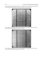
Fig. 8. Distribution of shearing stress
p’ along the glue layer with different t
1
(part curve)

-10-8-6-4-20246810
-0.25
-0.20
-0.15
-0.10
-0.05
0.00
0.05
0.10
0.15
0.20
0.25
q'
x''
L=4h2
L=6h2
L=10h2
L=15h2
L=20h2

Fig. 9. Distribution of shearing stress
q’ along the glue layer with different length for TPS tiles

4.3 The effects of the thickness of TPS tiles on peeling stress
The thickness of the tiles in TPS design was also a very important consideration.
The thickness of TPS tile thermal protection system in the design is also a very important
consideration. We should analyze the effect of the TPS tiles thickness on the shear and
normal stress of the layer. Let the working stress of the structure
P=20MPa, and E
1
=2E
2
,
L=10 h
2
, t
0
=20°C, t
j0
=177°C, t
1
=500°C. When h
1
/h
2
= 1/2, 1/3, 1/5, 1/8, by the above theory,
we also get the distribution of shear and normal stress, as shown Figures 11 and 12
respectively.
The Mechanics Analysis of Desquamation for
Thermal Protection System (TPS) Tiles of Spacecraft

191
-12 -10 -8 -6 -4 -2 0 2 4 6 8 10 12

-0.1
0.0
0.1
0.2
0.3
0.4
0.5
0.6
p'
x''
L=4h2
L=6h2
L=10h2
L=15h2
L=20h2

Fig. 10. Distribution of shearing stress
p’ along the glue layer with different length for TPS tiles

-6-5-4-3-2-10123456
-0.20
-0.15
-0.10
-0.05
0.00
0.05
0.10
0.15
0.20
q'

x''
h1=h2
h1=0.5h2
h1=0.1h2
h1=0.05h2

Fig. 11. Distribution of shearing stress
q’ along the glue layer with different thickness for
TPS tiles
4.4 The effects of the material of TPS tiles on peeling stress
The selected material is different in different spacecraft TPS.
For different thermal systems of spacecraft, the selection of protection tile material is also
different. Here, from a mechanical point of view, we study the effects of different material
on the thermal protection tiles peeling off, i.e. the adhesive layer stress, mainly considering
the effect of elastic modulus. Let the working stress of the structure
P=20MPa, and
h
1
/h
2
=0.5, L=10 h
2
,

t
0
=20=°C, t
j0
=177°C, t
1

=500°C. When E
1
/E
2
=0.5, 1, 2, and 3, by the above
theory, we also get the distribution of shear and normal stress, as shown Figures 13, 14 and
15 respectively.
Advances in Spacecraft Technologies

192



-6 -5 -4 -3 -2 -1 0 1 2 3 4 5 6
-0.5
0.0
0.5
1.0
1.5
2.0
2.5
p'
x''
h1=h2
h1=0.56h2
h1=0.1h2
h1=0.05h2


Fig. 12. Distribution of shearing stress p’ along the glue layer with different thickness for

TPS tiles



-5-4-3-2-1012345
-0.20
-0.15
-0.10
-0.05
0.00
0.05
0.10
0.15
0.20
q'
x''
E1=0.5E2
E1=E2
E1=2E2
E1=3Eh2


Fig. 13. Distribution of shearing stress
q’ along the glue layer with different materials for TPS
tiles
The Mechanics Analysis of Desquamation for
Thermal Protection System (TPS) Tiles of Spacecraft

193
-5 -4 -3 -2 -1 0 1 2 3 4 5

-0.05
0.00
0.05
0.10
0.15
0.20
0.25
0.30
0.35
0.40
p'
x''
E1=0.5E2
E1=E2
E1=2E2
E1=3E2

Fig. 14. Distribution of shearing stress
p’ along the glue layer with different materials for
TPS tiles

4.5 4.6 4.7 4.8 4.9 5.0 5.1
0.10
0.15
0.20
0.25
0.30
0.35

p'
x''
E1=0.5E2
E1=E2
E1=2E2
E1=3E2

Fig. 16. Distribution of shearing stress
p’ along the glue layer with different materials for
TPS tiles (part curve)
5. Conclusions
By analyzing the glue layer stress between TPS tiles and structures, and the influence of the
size and material of TPS tiles, we concludes:
1.
In the connection between TPS tiles and internal structure, the normal stress on the glue
layer end reaches the max value with naught shear stress. Hence, it can be indicated
that potential factors of the peeling off of the tiles are mainly contributed by peeling
normal stress and influenced little by shear stress.
Advances in Spacecraft Technologies

194
2. Glue layer stress concentrates near the edge of the tiles and almost naught in other
areas. The fact that the ratios of glue layer shear stress and normal stress to working
stress decreases with increasing working stress in the inner structure indicates that the
increasing rate of glue layer stress is less than that of working stress.
3.
Glue layer shear stress and normal stress both increases with temperature increasing,
however, the increasing magnitude is not very large compared to influence of working
stress’s increasing on peeling stress, which also illustrates that the more aerodynamic
heating is, the larger peeling stress of tiles is, quickening the desquamation of tiles.

4.
Glue layer shear stress and normal stress concentrates much more near the end of tiles
and their extremum get larger as the length of TPS tilse increases; furthermore, the
shear stress varies much more. This fact indicates that larger size of TPS tiles leads to
peeling stress of glue larger and the influence of the length of the TPS tiles on the
extremum of glue layer stress is obvious.
5.
However, glue layer stress does not decrease (or increase) as the thickness of TPS tiles
decreases (or increases). The thickness of TPS tiles does not influence the extremum of
glue layer shear stress obviously, but much glue layer normal stress.
6.
The influence of material Elastic modulus on peeling stress of glue layer is not strong,
however, as a whole, the larger material Elastic modulus (i.e. Stiffness) is, the larger
peeling stress of glue layer is.
6. References
XING Yu-zhe., 2003. The final investigation report of columbia disaster[J].Spece Exploration,
pp. 12:18-19.
Kuhn P., 1956.
Stress in Aircraft and Structures[M].McCraw-HIHLL BOOK COMPANY,
ZANG Qing-lai, ZHANG Xing, WU Guo-xun. (2006). New model and new method of stress
analysis about glued joints[J].
Chinese Journal of Aeronautics, pp.6:1051-1057.
Timoshenko S., 1958.
Strength of Materials[M].Van Nostrand Reinhold Company.
HU Hai-chang., 1980. Variational Principle and Application in Theory of Elasticity[M].
Beijing:Science Press.
ZHANG Xing (editor in chief)., 1995.
Advanced Theory of Elas-ticity [M]. Beijing:Beijing
University of Aeronautics and Astronautics Press.
QIAN Wei-chang., 1980.

Variational Method and finite Element[M].Beijing:Sci-enee Press.
The editorial department of Mechanical dic-tionary., 1990.
Mechanical Dietinary [M].
Beijing:Encyclopedia of China Publishing House, pp.197-597.
Davis J,Green, translsted by Gong Jiang-hong., 2003.
The Mechanical Properties Introduction of
Ceramic Materials
[M].Beijing:Tsinghua University Press, pp.21-35.]

Part 2
Cutting Edge State Estimation Techniques

10
Unscented Kalman Filtering for Hybrid
Estimation of Spacecraft Attitude Dynamics
and Rate Sensor Alignment
Hyun-Sam Myung
1
, Ki-Kyuk Yong
2
and Hyochoong Bang
1

1
Korea Advanced Institute of Science and Technology,

2
Korea Aerospace Research Institute,
Republic of Korea
1. Introduction

Requirements of highly precise pointing performance have been imposed on recently
developed spacecrafts for a variety of missions. The stringent requirements have called on
on-orbit estimation of spacecraft dynamics parameters and calibration of on-board sensors
as indispensible practices.
Consequently, on-orbit estimation of the mass moment of inertia of spacecraft has been a
major issue mostly due to the changes by solar panel deployment and a large portion of fuel
consumption (Creamer et al., 1996; Ahmed et al., 1998; Bordany et al., 2000; VanDyke et al.,
2004; Myung et al., 2007; Myung & Bang, 2008; Sekhavat et al., 2009).
As for measurement sensors, on-board calibration of alignment and bias errors of attitude and
rate sensors is one of the main concerns of attitude sensor calibration researches (Pittelkau,
2001 & 2002, Lai et al., 2003). Pittelkau (2002) proposed an attitude estimator based on the
Kalman filter (Kalman, 1960), in which spacecraft attitude quaternion, rate sensor
misalignment and bias, and star tracker misalignments are taken into consideration as states,
whereas the body rate is dealt as a synthesized signal by the estimates. Lai at al. (2003) derived
a method for alignment estimation of attitude and rate sensors based on the unscented Kalman
filter (UKF) (Julier and Uhlmann, 1997). Ma and Jiang (2005) presented spacecraft attitude
estimation and calibration based only magnetometer measurements using an UKF.
An interesting point is that we need predesigned 3-axis excitation manoeuvres of spacecraft
for both dynamics parameter estimation and sensor calibration. Therefore, this study is
motivated to merge above estimation and calibration processes into a single filtering
problem. It is noteworthy that poor information of moments of inertia is to be treated as a
system uncertainty while the rate sensor model errors are to be incorporated into the
measurement process.
As a filtering algorithm, this study employs a UKF. Extended Kalman filters (EKFs) have
been successfully applied to the nonlinear attitude estimation problem (Crassidis et al.,
2007). Hybrid estimation using the EKF has been reported by Myung at al. (2007). However,
the EKF estimates using the first order linearization, which may lead to instability of the
filter (ValDyke et al., 2004). The UKF approximates the nonlinear model to the second order
by spreading points 1 sigma apart from the a priori mean. Performing nonlinear
Advances in Spacecraft Technologies

198
transformation of sigma points produces the posterior mean and covariance. Despite the
computational burden of the UKF, extension of convergence region and numerical stability
greatly outperform the EKF.
Parameter estimation by a dual UKF was proposed by VanDyke et al. (2004). Since UKF has
more computational burden compared to EKF, a numerically efficient UKF was also
developed for state and parameter estimation (van der Merwe & Wan, 2001).
In this paper, the UKF is applied to simultaneous spacecraft dynamics estimation and rate
sensor alignment calibration using star tracker measurements. The spacecraft attitude and
the body angular velocity are the state vectors. Estimation parameters are the six
components of moment of inertia, and the bias, scale factor errors and misalignments of a
rate sensor. Numerical simulations compare the results to those using the EKF.
2. Equation of motion of spacecraft
2.1 Attitude representation
Spacecraft attitude parameter is the unit quaternion defined by

[]
[]
T
T
T
1234
T
13 4
q= sin cos
22
=q q q q
=q q
⎡

⎤φφ
⎛⎞ ⎛⎞
⎜⎟ ⎜⎟
⎢
⎥
⎝⎠ ⎝⎠
⎣
⎦
n
(1)
where n is the Euler axis and
φ
is the Euler angle. q
13
is the vector part and q
4
is the scalar
part in quaternion representation. Quaternion multiplication represents successive rotation
(Wertz, 1978)

43 211
34 12
2
2 1433
1234
4
q=q q
qq-qq
q
-q q q q q

=
q-qqq
q
-q -q -q q q
′
′′
⊗
′′′′
⎡⎤
⎡
⎤
⎢⎥
⎢
⎥
′′ ′′
⎢⎥
⎢
⎥
⎢⎥
⎢
⎥
′′′′
⎢⎥
⎢
⎥
′′′′
⎣
⎦
⎣⎦
(2)

And inverse of quaternion

[]
T
-1
1234
q = -q -q -q q (3)
implies the opposite rotation of q. By combining Eq. (2) and (3) residual rotation of q” with
respect to q’, or error quaternion δq, is obtained such as

()
-1
q=q q
δ
′
′′
⊗ (4)
2.2 Spacecraft attitude equation of motion
The equation of motion of spacecraft is given as
Jω + ω ×Jω =u

(5)
Unscented Kalman Filtering for Hybrid Estimation of Spacecraft
Attitude Dynamics and Rate Sensor Alignment

199
where
3
ω R∈
is the body angular velocity, J is the mass moment of inertia matrix, and

3
u R∈
is the external control input torque. The attitude kinematics is expressed by attitude
quaternion such as (Crassidis et al., 1997)


11
q= Ω(ω)q = Ξ(q)ω
22
(6)
where

,
×
⎡
⎤⎡ ⎤
≡≡
⎢
⎥⎢ ⎥
⎢
⎥⎢ ⎥
⎣
⎦⎣ ⎦
43 13
TT
13
-[ω×] ω qI +[q ]
Ω(ω) Ξ(q)
-ω 0-q
(7)

Due to the unity constraint on the attitude quaternion, only the vector component is utilized
as states, and q
4
is calculated from the constraint. Choosing the body angular rate as one of
the states, we rewrite Eq. (5) as


-1 -1
ω =-J ω×Jω+J u (8)
The six components of the moment of inertia are defined as

11 12 13
12 22 23
13 23 33
JJJ
J= J J J
JJJ
⎡
⎤
⎢
⎥
⎢
⎥
⎢
⎥
⎣
⎦
(9)
In the form of vector notation, we define

⎡
⎤
⎣
⎦
T
11 22 33 12 13 23
p = J J J J J J (10)
2.3 Measurement model
The body angular velocity measurement equation at time
k
t=t is expressed as

kkωk
ω =(I+M)ω +b+v

(11)
where ω is the true body angular velocity, ω

is the angular velocity measurement vector, M
is a matrix combined by the scale factor errors and the misalignments such as

11213
21 2 23
31 32 3
λδ δ
M= δλδ
δδ λ
⎡
⎤
⎢

⎥
⎢
⎥
⎢
⎥
⎣
⎦
(12)
where
3
b R∈ is the bias error vector. The scale factor and the misalignment are written in
vector form as

[]
[]
T
123
T
12 13 21 23 31 32
λ = λλλ
δ = δδδδδδ
(13)
Advances in Spacecraft Technologies

200
In this article, misalignment and bias error of the attitude sensor, usually given as a start
tracker, are not assumed because those of the star trackers are usually less than those of the
rate sensors.
3. Unscented Kalman filter
In this section, the unscented Kalman filter algorithm is presented. Ever since Julier and

Uhlmann have proposed the algorithm, numerous modifications and enhancements have
been reported. For estimation of parameters as well as state variables two methodologies are
mainly employed – joint and dual filtering techniques. Between the two methods, the joint
approach is easier and more intuitive to implement. Joint filters augment the original state
variables with parameters to be estimated. Since parameters are usually assumed to be
constant, time update of the filter model does not change the expanded parameter variables
except its process noise if assumed. On the contrary, the dual method set up another filter
for parameters so that two filters run sequentially in every step. The state estimator first
propagates and updates for given measurements, and then the parameter estimator updates
considering the updated output of the state variables as measurements. It is argued that the
primary benefit of the dual UKF is being able to prevent erratic behaviour by decoupling the
parameter filter from the state filter (VanDyke et al., 2004). However, the UKF in this
problem converges only with the joint method as shown later. This section summarizes the
UKF algorithm. This summary of the UKF equations follows the descriptions by Wan and
van der Merwe (2000) and VanDyke et al. (2004).
3.1 Joint estimation
The state variable and the parameter are noted by
n
∈sRs and
m
∈d R , respectively. The
augmented state variable of the joint filter is defined by

T
TT
x= s d
⎡
⎤
⎣
⎦

(14)
The filter initialization is conducted with assumed mean and covariance of the augmented
state vector.

{
}
()()
{}
00
x0 00 00
ˆˆ
x(t ) = E x
ˆˆ
P = E x(t ) - x x(t ) - x
T
(15)
Denoting
L=n+m, the sigma points of L are generated using the a priori mean and
covariance of the state as

k-1 k-1
T
TT T
k-1 k-1 k-1 x k-1 x
ˆˆ ˆ
χ =x x + (L+γ)P x - (L + γ)P
⎡
⎤
⎣
⎦

(16)
where
2
γ = α (L + κ)-Lis a scaling parameter. α is usually set to a small positive value. κ is a
secondary scaling parameter usually set to 0. The set of singular points,
k
χ
, is
×L(2L+1)

matrix. Defining
i, k
χ as ith column of
k
χ , each sigma point is propagated through the
nonlinear system

()
T
i, k|k-1 i, k-1 k-1
χ =F χ ,u (17)
Unscented Kalman Filtering for Hybrid Estimation of Spacecraft
Attitude Dynamics and Rate Sensor Alignment

201
The posterior mean,
ˆ
-
k
x , and the covariance,

−
xk
P, are determined from the statistics of the
propagated sigma points as follows:

()()
2L
-m
kii,k|k-1
i=0
2L
T
-c - -
xk i i,k|k-1 k i,k|k-1 k xk
i=0
ˆ
x= Wχ
ˆˆ
P= Wχ -x χ -x +Q
∑
∑
(18)
Q
xk
is the process noise covariance of the system. The weights,
m
i
W and
c
i

W , are calculated
by

m
0
c2
0
cm
ii
γ
W=
L+γ
γ
W= +1-α +β
L+γ
1
W=W = , i 1, ,2L
2(L + γ)
= "
(19)
β is used to incorporate prior knowledge. For Gaussian distributions, β = 2 is optimal. The
estimated measurement vector
ϒ
i, k|k -1
, ith column of matrix
(
)
(2 1)lL
R
×+

ϒ∈
k|k - 1
is calculated
by transforming the sigma points using the nonlinear measurement model,

(
)
χ
ϒ
i, k|k - 1 i, k|k - 1
= H (20)
The mean measurement,
ˆ
-
k
y
, and the measurement covariance,
y
k
y
k
P , are calculated based
on the statistics of the transformed sigma points.

()()
2L
m
kii,k|k-1
i=0
2L

T
c
ykyk i i, k | k -1 k i,k| k -1 k yk
i=0
ˆ
y= W
ˆˆ
P=W -y -y+R
ϒ
ϒϒ
∑
∑
(21)
R
y
k
is the measurement noise covariance matrix. The cross-correlation covariance,
xk
y
k
P, is
calculated using

()()
2L
T
c- -
xkyk i i,k |k -1 k i,k|k -1 k
i=0
ˆˆ

P=W -x -y
χ
ϒ
∑
(22)
The Kalman gain matrix is approximated from the cross-correlation and measurement
covariances using

-1
xk xkyk ykyk
K=PP (23)
The measurement update equations used to determine the mean,
ˆ
k
x , and covariance,
xk
P ,
of the filtered state are
Advances in Spacecraft Technologies

202

(
)

kk kkk
-T
xk xk xk ykyk xk
ˆˆ ˆ
x=x+K y-y

P=P-KP K
(24)
3.2 Joint UKF state variables
In this paper, the state vector of the original system consists of the attitude quaternion and
the angular rate. The attitude quaternion is a unique non-singular parameterization.
However, quaternion has to satisfy unity constraint of the magnitude, which may result in
covariance singularity if all the four elements are used. Therefore, only the vector
components will be used in the UKF implementation.
Parameters of to be estimated is six components of the moment of inertia, the scale factor
error, six elements of misalignment, and the bias of the rate sensor as in Eqs. (10), (12), and
(13). Therefore,

T
T TTTTT
13
x= δq ω p λδb
⎡
⎤
⎣
⎦
(25)
where

-1
ˆ
q=q q
δ
⊗
(26)
Since the error quaternion is utilized, the state is initialized with

T
TTTTTT
k-1 3 1 k-1 k-1 k-1 k-1 k-1
ˆ
x=0 ω p λδb
×
⎡
⎤
⎣
⎦
(27)
Once the sigma points are calculated, quaternion component
χ
13,i
δq
is used to obtain the
four-element sigma point quaternion
i
χ
q to propagate the nonlinear model.

13,i 13,i 13,i k -1
ˆ
q δq1δq δqq
T
T
i
χχ χχ
⎡⎤

=− ⊗
⎣⎦
(28)
The parameters are assumed to be constant.

0
0
0
0
p
b
λ
δ
=
=
=
=




(29)
Now, Eqs. (6), (8) and (29) constitute the nonlinear system model of the UKF. And, lastly the
following is the measurement equation.

13,k 13,k qk
δq=δq+v
kkωk
ω =(I+M)ω +b+v



(30)
After model propagation, three component of error quaternion is calculated again. After
measurement update of Eq. (24), four-element quaternion can be determined using

T
TT
k 13,k 13,k 13, k k -1
ˆˆ ˆˆ ˆ
q δq1δq δqq
⎡⎤
=− ⊗
⎣⎦
(31)
Unscented Kalman Filtering for Hybrid Estimation of Spacecraft
Attitude Dynamics and Rate Sensor Alignment

203
More detailed and helpful discussion on quaternion-based computation can refer (Kraft,
2003).
4. Numerical simulation results
In this section, simulation results for hybrid estimation of states, the moment of inertia and
the rate sensor calibration will be presented. The joint UKF will be compared to the results
using EKF (Myung et al., 2007).
4.1 Simulation conditions
In order to estimate the inertia matrix and the gyro calibration parameters, ‘persistent
excitation’ of motion should be guaranteed. A constant body angular velocity vector or one
with constant direction will not satisfy this requirement.
As one of the reference trajectories satisfying the ‘persistent excitation’ condition (Pittelkau,
2001), the following rate trajectory is proposed (Myung et al., 2007).

r
ω l-(1-cos )l l lsin
=
φφ×+φ


where
12
12
2
1
2
=50πt(rad)
sinω tsinω t
l= cosω tsinω t
cosω t
ω =0.01rad/s
ω =0.004rad/s
φ
⎡
⎤
⎢
⎥
⎢
⎥
⎢
⎥
⎣
⎦

For simulation purposes, a predictive controller (Crassidis et al., 1997) is applied to the
spacecraft attitude control. Given reference trajectories to follow, the predictive control
synthesizes control command based on nonlinear state prediction strategy using the Taylor
series expansion. The reference trajectories are shown in Fig. 1 and Fig. 2.
4.2 Simulation results
The following true system and alignment parameters are assumed (Myung et al., 2007):
⎡⎤
⎢⎥
⎢⎥
⎢⎥
⎣⎦
⎡⎤
⎣⎦
⎡⎤
⎣⎦
×
⎡⎤
⎣⎦
2
T
T
T
-4
200 50 -30
J = 50 240 10 kgm /s
-30 10 100
λ = 5000, -1000, -2000 ppm
δ = 648, 1296, 972, 648, -648, 1296 arcs
b = 5, 3, 2 10 rad /s

Advances in Spacecraft Technologies

204
0 5 10 15
-1
-0.8
-0.6
-0.4
-0.2
0
0.2
0.4
0.6
0.8
1
Quaternion reference trajectory
Quaternion
Time (min)


q
1
q
2
q
3
q
4

Fig. 1. Quaternion reference trajectory
0 5 10 15
-4
-3
-2
-1
0
1
2
3
4
Body rate reference trajectory
deg/s
Time (min)


ω
1
ω
2
ω
3

Fig. 2. Body angular rate reference trajectory
Unscented Kalman Filtering for Hybrid Estimation of Spacecraft
Attitude Dynamics and Rate Sensor Alignment

205
Nominal values of the parameters are given as
⎡⎤

⎢⎥
⎢⎥
⎢⎥
⎣⎦
⎡⎤
⎣⎦
⎡⎤
⎣⎦
⎡⎤
⎣⎦
2
T
T
T
160 20 -20
J = 20 160 -20 k
g
m/s
-20 -20 160
λ = 0 0 0 ppm
δ =000000arcs
b= 0 0 0 rad/s

The process and the measurement noise covariance matrices are designated as
33
33
33
×
×
×

-8 2 4
-6 2
q
-5 2 2
ω
Q = 10 I rad /s
R = 10 I rad
R = 10 I rad /s

Simulation is performed for 15 min. The star tracker and the rate sensor measurements are
assumed to be given every 0.2 s. Table 1 – 4 present estimation error comparison of the EKF
and UKF by Monte-Carlo simulation of 20 runs. The upper data in each cell of the tables are
percentage error with respect to own value. The lower data are normalized values of the
final covariances. Therefore, smaller values are more accurate
regardless of magnitude of
the nominal parameter values. The moment of inertia estimation is very accurate for both
EKF and UKF in Table 1. However, rate sensor calibration results of the UKF are much more
accurate than those of EKF. If the reference trajectory is designed considering excitation
optimality, estimation results will be even more accurate (Sekhavat, 2009).

units J
11
J
22
J
33
J
12
J
13

J
23

(1σ) (1σ) (1σ) (1σ) (1σ) (1σ)
EKF % error 0.140 0.163 0.527 0.137 0.319 0.548
% (0.106) (0.096) (0.250) (0.279) (0.310) (0.847)
UKF % error 0.080 0.073 0.185 0.072 0.023 0.063
% (0.879) (0.788) (1.793) (0.832) (1.577) (4.495)
Table 1. Moment of inertia estimation results of EKF and UKF by Monte-Carlo Simulation

units
λ
1

(1σ)
λ
2

(1σ)
λ
3

(1σ)
EKF
% error
%
53.9
(82.4)
56.3
(205.6)

13.7
(117.0)
UKF
% error
%
1.17
(32.0)
61.8
(138.0)
18.8
(55.3)
Table 2. Rate sensor scale factor error estimation results of EKF and UKF by Monte-Carlo
Simulation
Advances in Spacecraft Technologies

206
units δ
12
δ
13
δ
21
δ
23
δ
31
δ
32

(1σ) (1σ) (1σ) (1σ) (1σ) (1σ)

EKF % error 91.2 121.9 72.0 103.8 59.6 14.0
% (87.1) (47.6) (75.0) (72.9) (85.0) (64.1)
UKF % error 28.3 6.81 13.5 7.74 6.51 10.9
% (49.3) (18.3) (32.9) (34.3) (46.2) (26.9)
Table 3. Rate sensor misalignment estimation results of EKF and UKF by Monte-Carlo
Simulation
units
b
1

(1σ)
b
2

(1σ)
b
3

(1σ)
EKF
% error
%
267.1
(29.6)
166.1
(47.6)
37.7
(67.9)
UKF
% error

%
2.46
(9.63)
11.6
(16.0)
1.93
(23.8)
Table 4. Rate sensor bias estimation results of EKF and UKF by Monte-Carlo Simulation
Fig. 3 to Fig. 10 illustrates one of the UKF simulation results with time. Each variable has
different convergence time constant. The attitude and the rate converge very fast as in Fig. 3
and Fig. 4. And then the moment of inertia components converge. And finally calibration
parameters converge.

0 5 10 15
-2
0
2
x 10
-3
Error Quaternion
q
1


Meas
Est
3
σ
0 5 10 15
-2

0
2
x 10
-3
q
2
0 5 10 15
-2
0
2
x 10
-3
q
3
Time (min)

Fig. 3. Attitude estimation error with 3σ bounds
Unscented Kalman Filtering for Hybrid Estimation of Spacecraft
Attitude Dynamics and Rate Sensor Alignment

207
0 5 10 15
-0.5
0
0.5
Body angular rates


Meas
Est

3
σ
0 5 10 15
-0.5
0
0.5
ω
3
(deg/s)
0 5 10 15
-0.5
0
0.5
ω
3
Time (min)

Fig. 4. Angular velocity estimation error with 3σ bounds

0 5 10 15
100
-80
-60
-40
-20
0
20
40
60
80

Time (min)
Moment of inertia error


Δ
J
11
Δ
J
22
Δ
J
33
Δ
J
12
Δ
J
13
Δ
J
23

Fig. 5. Moment of inertia estimation error
Advances in Spacecraft Technologies

208
0 5 10 15
-20
-10

0
10
20
J
11
0 5 10 15
-20
-10
0
10
20
J
22


0 5 10 15
-20
-10
0
10
20
J
33
0 5 10 15
-20
-10
0
10
20
J

12
0 5 10 15
-20
-10
0
10
20
J
13
Time (min)
0 5 10 15
-20
-10
0
10
20
J
23
Time (min)

Fig. 6. Moment of inertia estimation error with 3σ bounds

0 5 10 15
-10
-5
0
5
x 10
-3
SF

Parameter estimation error
0 5 10 15
-0.01
-0.005
0
0.005
0.01
MIS
0 5 10 15
-1
-0.5
0
0.5
1
x 10
-3
Bias
Time (min)

Fig. 7. Rate sensor calibration error
Unscented Kalman Filtering for Hybrid Estimation of Spacecraft
Attitude Dynamics and Rate Sensor Alignment

209
0 5 10 15
-2
-1
0
1
2

x 10
4
λ
1
(ppm)
0 5 10 15
-1
-0.5
0
0.5
1
x 10
4
λ
2
(ppm)
0 5 10 15
-1
-0.5
0
0.5
1
x 10
4
λ
3
(ppm)
Time (min)

Fig. 8. Rate gyro scale factor estimation error with 3σ bounds

0 5 10 15
-4000
-2000
0
2000
4000
δ
12
(arcsec)
0 5 10 15
-4000
-2000
0
2000
4000
δ
13
(arcsec)
0 5 10 15
-4000
-2000
0
2000
4000
δ
21
(arcsec)
0 5 10 15
-4000

-2000
0
2000
4000
δ
23
(arcsec)
0 5 10 15
-4000
-2000
0
2000
4000
δ
31
(arcsec)
Time (min)
0 5 10 15
-4000
-2000
0
2000
4000
δ
32
(arcsec)
Time (min)

Fig. 9. Rate gyro misalignment estimation error with 3σ bounds
Advances in Spacecraft Technologies

210
0 5 10 15
-2
-1
0
1
2
x 10
-3
b
1
0 5 10 15
-2
-1
0
1
2
x 10
-3
b
2
0 5 10 15
-2
-1
0
1
2
x 10
-3

b
3
Time (min)

Fig. 10. Rate gyro bias estimation error with 3σ bounds
5. Conclusions
This study presented hybrid estimation of the moment of inertia of spacecraft and
calibration parameters of the rate sensor such as the scale factor error, six elements of
misalignment and the gyro bias error during a single estimation maneuver. For this
purpose, a joint unscented Kalman filter (UKF) algorithm was successfully applied and the
performance was compared to the results using the extended Kalman filter (EKF). While the
components of the moment of inertia were estimated very accurately by both the EKF and
the UKF, the rate sensor calibration parameters – scale factor, misalignment, and bias error –
were filtered much better by the UKF than the EKF. Simulation results demonstrated
applicability and performance for spacecraft system identification and the gyro calibration
simultaneously.
This concept of estimation procedure can reduce efforts and costs for periodic parameter
estimation and gyro calibration of spacecraft in-orbit. Also, proposed method can be
extended to calibration maneuvers of other equipments such as star trackers and optical
payloads.
6. References
Ahmed, J.; Coppola, V. T. & Bernstein, D. S. (1998). Adaptive asymptotic tracking of
spacecraft attitude motion with inertia matrix identification,
Journal of Guidance,
Control and Dynamics, Vol. 21, No. 5, pp. 684-691
Unscented Kalman Filtering for Hybrid Estimation of Spacecraft
Attitude Dynamics and Rate Sensor Alignment

211
Bordany, R. E.; Steyn, W. H. & Crawford, M. (2000). In-orbit estimation of the inertia matrix

and thruster parameters of UoSat-12,
Proceedings of the 14th AIAA/USU Conference
on Small Satellites
, Logan, Utah, USA, August 2000
Crassidis, J. L.; Markley, F. L., Anthony, T. C. & Andrews, S. F. (1997). Nonlinear predictive
control of spacecraft
, Journal of Guidance, Control and Dynamics, Vol. 20, No. 6, pp.
1096-1103
Crassidis, J. L.; Markley, F. L. & Cheng, Y. (2007). Survey of nonlinear attitude estimation
methods,
Journal of Guidance, Control and Dynamics, Vol. 30, No. 1, pp. 12-28
Creamer, G.; DeLaHunt, P., Gates, S. & Leyenson, M. (1996). Attitude determination and
control of Clementine during lunar mapping,
Journal of Guidance, Control and
Dynamics
, Vol. 19, No. 3, pp. 505-511
Julier, S. J. & Uhlmann, J. K. (1997). A new extension of the kalman filter to nonlinear
systems,
Proceedings of the SPIE AeroSense International Symposium on
Aerospace/Defence Sensing, Simulation and Controls
, Orlando, Florida, USA, April
1997
Kalman, R. E. (1960). A new approach to linear filtering and prediction problems,
Transactions of the ASME-Journal of Basic Engineering, D, Vol. 82, pp. 35-45
Kraft, E. (2003). A quaternion-based uscented Kalman filter for orientation tracking,
Proceedings of IEEE 6th Coference of Information Fusion, pp. 47-54
Lai, K. L.; Crassidis, J. L. & Harman, R. R. (2003). In-space spacecraft alignment calibration
using the unscented filter,
Proceedings of AIAA Guidance, Navigation, and Control
Conference Exhibit

, Austin, Texas, USA, August 2003
Ma, G. -F. & Jiang, X. -Y. (2005). Unscented Kalman filter for spacecraft attitude estimation
and calibration using magnetometer measurements,
Proceedings of the 4th
International Conference on Machine Learning and Cybernatics
, Guanzhou, August 2005
Myung, H.; Yong, K. -L. & Bang, H. (2007). Hybrid estimation of spacecraft attitude
dynamics and rate sensor alignment parameters,
Proceedings of International
Conference on Control, Automation and Systems
, Seoul, Korea, October 2007
Myung, H. & Bang, H. (2008). Spacecraft parameter estimation by using predictive filter
algorithm,
Proceedings of IFAC World Congress, Seoul, Korea, July 2008
Pittelkau, M. E. (2001). Kalman filtering for spacecraft system alignment calibration,
Journal
of Guidance, Control and Dynamics
, Vol. 24, No. 6, pp. 1187-1195
Pittelkau, M. E. (2002), Everything is relative in spacecraft system alignment calibration,
Journal of Spacecraft and Rockets, Vol. 39, No. 3, pp. 460-466
Sekhavat, P. ; Karpenko, M. & Ross, I. M. (2009). UKF-based spacecraft parameter estimation
using optimal excitation,
AIAA Guidance, Navigation, and Control Conference,
Chicago, Illinois, USA, August 2009
Van der Merwe, R. & Wan, E. A. (2001). The squre-root unscented Kalman filter for state and
parameter-estimation,
Proceedings of IEEE International Conference on Acoustics,
Speech, and Signal Processing
, Vol. 6, pp. 3461-3464
VanDyke, M. C.; Schwartz, J. L. & Hall, C. D. (2004). Unscented Kalman filtering for

spacecraft attitude state and parameter estimation,
Advances in the Astronautical
Sciences
, Vol. 118, No. 1, pp. 217-228
Advances in Spacecraft Technologies

212
Wan, E. A. & van der Merwe, R. (2000). The unscented Kalman filter for nonlinear
estimation,
Proceedings of IEEE Symposium 2000 (AS-SPCC), Lake Louise, Alberta,
Canada, October 2000
Wertz, J. R. (Ed.) (1978).
Spacecraft Attitude Determination and Control, pp. 414-416, Kluwer

11
Fault-Tolerant Attitude Estimation for Satellite
using Federated Unscented Kalman Filter
Jonghee Bae, Seungho Yoon, and Youdan Kim
School of Mechanical and Aerospace Engineering, Seoul National University,
Republic of Korea
1. Introduction
Satellites provide various services essential to the modern life of human being. For example,
satellite images are used for many applications such as reconnaissance, geographic
information system, etc. Therefore, design and operation requirements of the satellite
system have become more severe, and also the system reliability during the operation is
required. Satellite attitude control systems including sensors and actuators are critical
subsystems, and any fault in the satellite control system can result in serious problems. To
deal with this problem, various attitude estimation algorithms using multiple sensors have
been actively studied for fault tolerant satellite system (Edelmayer & Miranda, 2007;
Jiancheng & Ali, 2005; Karlgaard & Schaub, 2008; Kerr, 1987; Xu, 2009).

Satellites use various attitude sensors such as gyroscopes, sun sensors, star sensors,
magnetometers, and so on. With these sensors, satellite attitude information can be obtained
using the estimation algorithms including Kalman filter, extended Kalman filter (EKF),
unscented Kalman filter (UKF), and particle filter. Agrawal et al. and Nagendra et al.
presented the attitude estimation algorithm based on Kalman filter for satellite system
(Agrawal & Palermo, 2002; Nagendra et al., 2002). Mehra and Bayard dealt with the
problems of satellite attitude estimation based on the EKF algorithm using the gyroscope
and star tracker as attitude sensors (Mehra & Bayard, 1995). In the EKF algorithm, the
nonlinearities of the satellite system are approximated by the first-order Taylor series
expansion, and therefore it sometimes provides undesired estimates when the system has
severe nonlinearities. Recently, researches on UKF have been performed because the UKF
can capture the posterior mean and covariance to the third order of nonlinear system. It is
known that the UKF can provide better results for the estimation of highly nonlinear
systems than EKF (Crassidis & Markley, 2003; Jin et al., 2008; Julier & Uhlmann, 2004).
Crassidis and Markley proposed the attitude estimation algorithm based on unscented filter,
and showed that the fast convergence can be obtained even with inaccurate initial
conditions. The UKF was used to solve the relative attitude estimation problem using the
modified Rodrigure parameter (MRP), where the gyroscope, star tracker, and laser
rendezvous radar were employed as the attitude sensors (Jin et al., 2008).
For multi-sensor systems, there are two different filter schemes for the measured sensor data
process: centralized Kalman fileter (CKF) and decentralized Kalman filter (DKF) (Kim &
Hong, 2003). In the CKF, all measured sensor data are processed in the center site, and