Advances in Vehicular Networking Technologies Part 7 potx

10
-4
10
-3
10
-2
10
-1
10
0
0 5 10 15 20 25 30 35 40 45
Pe
P (dB)
non-cooperative
NAF
hybrid NAF
hybrid OAF
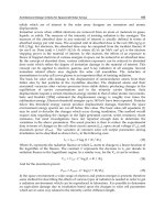
Fig. 4. Outage probabilities for the non-cooperative, NAF, Hybrid-NAF and Hybrid OAF
scheme. Considered information rates: 2 and 4 BPCU.
advantages in adopting an OAF hybrid cooperation protocol. First, the cooperation
complexity and cost are reduced. Second, the hybrid strategy reduces significantly the
complexity of the algorithm implemented to determine the outage probability. This is the
key reason for which we succeeded in finding an optimal power allocation algorithm for OAF
hybrid cooperation schemes. We now show some simulation results for hybrid cooperative
transmission without power allocation. Performance is compared in terms of average outage
probability versus average SNR.
Based on these mutual information expressions, we numerically compare non-cooperative,
NAF cooperative, hybrid NAF cooperative and hybrid OAF cooperative protocols in terms
of outage probability versus average SNR. Let
O

d
denotes the direct channel outage event,
O
d
= {I
d
< R},andO
c
denotes the cooperative channel outage event, O
c
= {I
c
< R}.The
equivalent channel is in outage if both events,
O
d
and O
c
, are realized.
Other simulation results are shown in Figure 4 for the case of one active relay and transmission
rate of 2 and 4 bits per channel use (BPCU). We find out that, adopting the proposed
OAF hybrid cooperation protocol, transmission outage performance is better than for both
non-cooperative and NAF hybrid cooperation transmissions. This result confirms our choice
of using an orthogonal scheme: since the channel is assumed to be quasi-static, if the direct
link is in outage in the first slot, it will remain in outage in the second one. The outage
performance improvement is not our major achievement. Combining hybrid cooperation with
OAF scheme, we obtain a cooperation protocol with both reduced complexity and cooperation
cost. Furthermore, the proposed hybrid strategy permits to reduce the complexity of the
outage probability computation. This is the key reason for which we succeeded in finding
an optimal power allocation algorithm only for OAF hybrid cooperation schemes.

172
Advances in Vehicular Networking Technologies
The Orthogonal AF strategy, sub-optimal in a full time cooperation scheme, is optimal with
the hybrid strategy. In fact, since the channels are assumed to be slow fading, if the direct link
is in outage in the first slot of the frame, it will be the case in the second. So it is better not to
transmit in the second slot, and thus economize power, since we are sure that the reliability of
the information is not guarantied. The mutual information is in this case
I
OAF
=
1
2
log
2
(1 + P
s
|f |
2
+
P
s
P
r
|bgh|
2
1 + P
r
|bg|
2
) (1)

4.2 Proposed Adaptive Modulation and Coding Combined with the Hybrid Cooperation
Protocol
In this section we present the mechanism proposed in (E. Calvanese Strinati and S. Yang and
J-C. Belfiore, 2007) in which the authors propose to combine the hybrid cooperation protocol
with an AMC mechanism. The protocol is named hybrid cooperative AMC mechanism. A flow
chart of the proposed algorithm is shown in Fig. 5. I
non−coop
is the instantaneous mutual
information when transmission is done in non-cooperative mode and R is the transmission
rate.
The algorithm is summarized as follows:
Step 1: S sends a RTS each time it wants to transmit new data.
Step 2: After receiving a RTS, the AMC mechanism (in D) selects R for next data transmission.
R is selected from the set of LUT of PER versus LQM for hybrid cooperation transmission
performance, given the LQM computed at previous received packet.
Step 3: D estimates the instantaneous channel conditions of the direct source-destination link
(σ
2
, f , etc.) and computes I
non−coop
( f , σ
2
)
Step 4: The cooperation controller in D decides if cooperate or not:
-ifI
non−coop
< R, non-cooperative transmission is forecasted to be in outage: the
cooperation controller starts cooperation (go to step 5)
- otherwise, cooperation mode is not activated (go to step 9)
Step 5: D checks if the relay probing is up to date:

-YES(gotostep9)
- NOT(gotostep6)
Step 6: relay probing: D probes the relays available for cooperation and estimates the channel
coefficients of the cooperation links.
Step7and8:Each relay calculates the product gain
|g
i
h
i
| and reacts by sending an availability
frame after t
i
time which is anti-proportional to |g
i
h
i
|. Therefore, the relay with the strongest
product gain is identified as relay 1, and so on.
Step 9: D sends a clear to send (CTS) that includes information on transmission rate R, M, relay
identifiers, etc.
Step 10: S starts data transmission at rate R
Step 11: After receiving data from S, D derives PER
pred
from the LUT of hybrid cooperation
and selects R for next transmission of S.
Summarizing, based on the direct source-destination link quality, a cooperation controller
decides if and how cooperate. We call this cooperation protocol as hybrid cooperation. The rate
173
Hybrid Cooperation Techniques
R is chosen after each received packet by the AMC that aims at maximizing the throughput

performance of the hybrid transmission mode meeting the QoS constraints imposed by the
upper layers.
Note that the AMC mechanism selects R based on a set of pre-computed AMC switching
points that depends on N, M, PER
target
, transmission scenario, etc. Such switching points
are chosen based on the average PER versus average performance of the hybrid cooperation
protocol. Given N, M and R, there is a crossing point (PER
cro s s
) between non-cooperative
and cooperative average performance. For PER
≤ PER
cro s s
cooperation outperforms
non-cooperative mode. Hence the gain of hybrid cooperation is high since the direct
link results more often in outage that cooperative transmission. When PER
> PER
cro s s
,
non-cooperative transmission outperforms cooperation. In such case the gain of hybrid
cooperation is reduced and asymptotically (for PER
cro s s
→ 0) hybrid cooperation performs
as non-cooperative transmission since cooperation is never activated. In order to fully exploit
the proposed hybrid cooperative AMC to improve the average system performance, AMC
mechanism and hybrid cooperation protocol have to be designed jointly. As an example,
given our system model, we computed the minimum values of M (M
min
)forwhichhybrid
cooperative AMC outperforms both classical non-cooperative and cooperative AMC. A

selection of our results are shown on table 1 for maximum transmission rates R
max
at which
the system can operate and typical PER
target
values imposed to the AMC. Indeed, given
N M
min
PER
target
R
max
2 9 10
−1
10
2 5 10
−2
10
2 7 10
−1
8
2 3 10
−2
8
2 5 10
−1
6
2 3 10
−2
6

2 5 10
−1
4
2 3 10
−2
4
2 3 10
−1
2
2 3 10
−2
2
Table 1. Minimum values of M (M
min
)fortypicalPER
target
values
PER
target
and R
max
,wecandefineanM
min
from which hybrid cooperation is beneficial. Note
that the larger M is the more complex the cooperation protocol is. There is indeed a trade off
between cooperation performance and cooperation complexity.
4.2.1 Simulation results
In this section, we show by means of numerical simulations the effectiveness of combining
the hybrid cooperation protocol with the AMC mechanism. Results first show how the
proposed mechanism drives to improved average system throughput performance. Then, we

outline the advantage introduced by the hybrid cooperation protocol in terms of reduction of
cooperation signalling overhead, cooperation protocol delay and average power consumed
by the active relays. Simulation results are given here for the system model presented
in section 3. In the system both AMC and ARQ are implemented. The simulated AMC
algorithm selects the MCS which maximizes the throughput while meeting the PER
target
174
Advances in Vehicular Networking Technologies
D: I
non-coop
≥ R
D: channel estimation
up to date?
D: compute I
non-coop
(ˆσ
2
z
)
D: rate R selected based
on the LQM
S:
→RTS
D: relay probing
Available relays
answer in order
D: selection of the best relays
D:
→ CTS(R,M,relay identifiers,etc.)
S: starts transmission

D: PER prediction
Yes
Yes
No
No
1
2
3
4
5
6
7
8
9
10
11
Fig. 5. Flow chart of the proposed hybrid opportunistic cooperation combined with AMC
175
Hybrid Cooperation Techniques
0 5 10 15 20 25 30 35 40
0
1
2
3
4
5
6
7
8
SNR dB

R ⋅ (1−PER)
cooperative
non−cooperative
hybrid
Fig. 6. Cooperative/non-cooperative/hybrid cooperative transmission with N = 2,M = 3
and PER
target
= 10
−2
QoS constraints. The set of MCS corresponds to the transmission rate set R=1,2,4,6,8.We fix
the PER
target
= 10
−2
. Moreover, a total average power constraint is imposed and no power
allocation is considered here. We access the average physical layer throughput of a system
that can perform data transmission with three different transmission modes: non-cooperative,
cooperative and hybrid. Performance is compared in terms of average throughput versus
average SNR. The link between source, destination and relays are assumed to be symmetric
and with independent fading coefficients.
On Fig. 6 we show the performance of the AMC algorithm combined with cooperation for
N
= 2andM = 3. From these results, we observe three regions for the SNR : the low, medium
and high SNR regions. At low SNR, the non-cooperation mode outperforms cooperation mode
since the noise power dominates the received power at the relays. In the medium SNR region,
the cooperative scheme outperforms the non-cooperative scheme with a gain up to 6 dB. This
gain is due to the better diversity-multiplexing trade-off (DMT) of the cooperative scheme.
However, this gain decreases for increasing SNR since we fix PER
target
= 10

−2
while R
max
= 8
and M
= 3 (hence M < M
min
, see table 1). Therefore, when M < M
min
, the cooperative
scheme is not preferable at high SNR.
On Fig. 7 the performance of the case N
= 2andM = 5isshown.Asdemonstratedin(S.Yang
and J-C. Belfiore, 2006), the DMT is improved with the number of slots M. This improvement
translates into a better performance in both cases. We observe that the decrease of SNR gain
at medium to high SNR is slower than the previous case. Cooperation is always better than
the non-cooperation since M
≥ M
min
. Best performance is always reached when using hybrid
cooperation. We remark that the hybrid scheme alleviates the performance loss of cooperation
176
Advances in Vehicular Networking Technologies
0 5 10 15 20 25 30 35 40
0
1
2
3
4
5

6
7
8
SNR dB
R ⋅ (1−PER)
cooperative
non−cooperative
hybrid
Fig. 7. Cooperative/non-cooperative/hybrid cooperative transmission with N = 2,M = 5
and PER
target
= 10
−2
in both the low SNR and the high SNR regions. In case of M = 3andM = 5, we observe
respectively up to 5 and 7.5 dB of gap from fixed-cooperation and 1.5 and 2 dB of gap from
non-cooperative transmission.
Hereafter we enlarge the investigation on hybrid cooperation protocols performance for a
realistic communication scenario such as, OFDMA based wireless mobile communication
transmission which employs limited modulation alphabets and real FEC codes. We access
the effectiveness of hybrid cooperation protocol in real communication scenarios in terms of
average PER versus average SNR, average system throughput enhancement and average
cooperation cost reduction. The set of parameters used in this simulations are chosen
according to the IEEE 802.16e standard . The mobile wireless channel is modelled according
to (Spatial Channel Model Ad Hoc Group, 2003).
We propose to use an OAF hybrid cooperation protocol under the following power constraint:
we impose a total average power constraint and no power allocation is considered. If P
denotes the total power constraint, we impose P
s
= P/2forthepowerallocatedtothe
source in the first slot and P

r
= P/2 the power allocated to the relay in the second slot.
Hereafter we adopt the following graphical notation: we represent respectively with the solid
blue line, dashed red line and solid green line, non-cooperative, persistent cooperative and
hybrid cooperative transmission mode performance.
Simulation results are given here for the system model presented in section 3. We use as
Forward Error Correcting (FEC) code the LDPC codes as specified by the standard IEEE
802.16e (IEEE Standards Department, 2005) for the different coding rates.
177
Hybrid Cooperation Techniques
8 10 12 14 16 18 20 22 24 26 28
10
−3
10
−2
10
−1
10
0
SNR dB
PER
Persistent Cooperation
Non Cooperation
Hybrid Cooperation
64 QAM 2/3
64 QAM 3/4
64 QAM 1/2
Fig. 8. Cooperative/non-cooperative/hybrid cooperative transmission
On figure 8 we compare the three transmission mode performance in terms of average PER
performance versus average SNR. Results are reported here only for 64-QAM modulation

with coding rates R
c
= 1/2, 2/3, 3/4. From these results, we observe that there is a
crossing point (PER
cross
) between non-cooperative and cooperative average performance.
For PER
≤ PER
cross
cooperation outperforms non-cooperative mode. Hence the gain of
hybrid cooperation is high since the direct link results more often in outage that cooperative
transmission. Note that the PER that corresponds to this crossing point depends on the code
correcting power: stronger codes present the crossing point at higher PER. For sake of simplicity
we impose same codeword length for each MCS. Therefore, the information block length is
larger for higher coding rate which results in a stronger correcting code. This is verified on
figure 8. When PER
> PER
cross
, non-cooperative transmission outperforms cooperation.
When PER
cross
→ 0, hybrid cooperation performs as non-cooperative transmission since
cooperation is never activated. Hybrid cooperation notably outperforms both cooperative
and non-cooperative transmissions for PER values close to PER
cross
. Note that in the
present simulation we also introduce a feedback delay between MI
non−coop
estimation and
cooperation controller action. Due to this delay, hybrid cooperation performance is slightly

decreased comparing to equivalent results presented in (E. Calvanese Strinati and S. Yang and
J-C. Belfiore, 2007).
In order to show the effectiveness of hybrid cooperative AMC mechanism, which combines
AMC with hybrid cooperation, we compare the three transmission modes in terms of average
system throughput versus average SNR. The simulated AMC algorithm selects the MCS
which maximizes the throughput while meeting the PER
target
QoS constraints (Calvanese
178
Advances in Vehicular Networking Technologies
Strinati E., 2006). Typical values for the target PER is a few percent. For instance, imposing
PER
target
≤ 10
−1
results in a residual PER below 10
−5
after 4 retransmissions.
The set of MCS corresponds to the transmission rate set defined by the IEEE 802.16e standard.
In our simulation results we show the per-user performance, having one data region of 24
sub-carriers (in frequency) and 16 data OFDM symbols (in time). Under this assumption, the
set of MCS schemes and the related nominal throughputs r
mcs
and information block lengths
N
Info
are given in table 2.
Modulation Code Rate N
Info
r

mcs
QPSK 1/2 384 (bits) 215 (Kb/s)
QPSK 3/4 576 (bits) 315 (Kb/s)
16-QAM 1/2 768 (bits) 420 (Kb/s)
16-QAM 3/4 1152 (bits) 630 (Kb/s)
64-QAM 1/2 1152 (bits) 630 (Kb/s)
64-QAM 2/3 1536 (bits) 840 (Kb/s)
64-QAM 3/4 1728 (bits) 945 (Kb/s)
Table 2. Modulation and Coding Schemes of IEEE 802.16e
When PER
target
< PER
cross
, then cooperation is always better than the non-cooperation.
Otherwise, non-cooperation transmission can outperform persistent cooperation
transmission. As an example, we report respectively on figure 10 and 9 our simulation
results for PER
target
= 10
−1
,5·10
−2
.
As it is shown on figure 9, with PER
target
= 5 ·10
−2
, persistent cooperation outperforms
non-cooperative transmission over all the considered SNR range since, PER
target

< PER
cross
for all MCS.
In this case, hybrid cooperation outperforms non-cooperative and persistent cooperative
transmission respectively with a gain up to 1.75 dB and 0.75 dB. Relaxing the constraint on the
PER
target
to PER
target
= 10
−1
, there are some MCS for which PER
target
> PER
cross
.Asa
consequence, non-cooperation outperforms persistent cooperation in same parts of the considered
SNR range. Again, hybrid cooperation outperforms non-cooperative and persistent cooperative
transmission respectively with a gain up to 1.25 dB and 0.9 dB (see figure 10).
We report hereafter also some simulation results aimed at understanding the average relaying
activation ratio χ) - which is the ratio between the number of frames were the relay is active
over the total number of transmitted frames - versus the average SNR adopting the proposed
hybrid cooperation protocol. Results are shown on Fig 11 for PER
target
= 10
−1
. Two working
zones of an AMC mechanism can be distinguished. In the first zone, even if AMC selects the
minimum MCS at which the system can operate, we have that PER
> PER

target
. Therefore,
since PER is large, χ is large too. For such link quality conditions the AMC may decide to avoid
transmission since AMC cannot assure the QoS constraints imposed by the upper layers. The
second zone starts when MCS selected for transmission assures PER
≤ PER
target
.Inthis
zone each saw tooth corresponds to a change of MCS. Our results outline that when AMC
can assure a PER
≤ PER
target
, χ is very small (χ ≤ PER
target
) since the hybrid cooperation
protocol activates the cooperative mode only when direct link transmission is in outage. At
the end of the second zone transmission is done at the highest MCS and the system operates
at PER
 PER
target
,withconsequentχ  1. Note that, contrary to the cooperative AMC
protocol case for which χ
= 1 over the whole SNR range, when AMC can assure a PER ≤
PER
target
and the proposed hybrid cooperation protocol is adopted, χ is reduced to the same
179
Hybrid Cooperation Techniques
0 5 10 15 20 25 30
0

100
200
300
400
500
600
700
800
900
SNR dB
Throughput (Kb/s)
Persistent Cooperative Transmission
Non Cooperative Transmission
Hybrid Cooperative Transmission
Fig. 9. Cooperative/non-cooperative/hybrid cooperative transmission with
PER
target
= 5 ·10
−2
order of magnitude of PER
target
. Note that the major result in our investigation is reduction of
average relaying activation and not the improvement in average system throughput achieved
with hybrid cooperative AMC mechanism.
The reduction of average relaying activation ratio achieved with the proposed hybrid AMC
protocol presents three main advantages. First, the average power consumed by the active
relays is strongly reduced especially when cooperation does not help and consequently
cooperation activation results in a waist of relays processing power. Second, the delay
caused by the cooperation protocol and consequently the packet delivery delay can be
strongly reduced adopting our proposed hybrid cooperation protocol. For instance, when

direct non-cooperative transmission is not forecasted to be in outage, the destination can
immediately send a clear to send (CTS), without waiting for the relay probing process. This
is an important attribute for scheduling algorithm with delay QoS constraints. Third, the
average computing complexity is reduced by decreasing the number of average operation
associated to cooperation.
4.3 An efficient power allocation optimization for hybrid cooperation protocols
In this section we combine the OAF hybrid cooperation protocol presented in section 4.1 with
an optimal power allocation algorithm. The goal is to maximize the mutual information of the
equivalent cooperative channel via optimal power allocation between the source and the relay.
It is well known that the performance of a cooperative scheme is improved by relaying with
optimal power values. Hereafter we assume that a maximal overall transmit power is fixed
by using, for instance, a suitable power control algorithm in order to minimize co-channel
180
Advances in Vehicular Networking Technologies
0 5 10 15 20 25 30
0
100
200
300
400
500
600
700
800
900
SNR dB
Throughput (Kb/s)
Persistent Cooperative Transmission
Non Cooperative Transmission
Hybrid Cooperative Transmission

Fig. 10. Cooperative/non-cooperative/hybrid cooperative transmission with
PER
target
= 10
−1
interference. The overall total transmitting power should then be optimally shared between
the source and the relay. The simplicity of an OAF cooperation scheme leads to an outage
probability expression easier to handle than in the NAF case. Basically, we optimize the power
allocation by minimizing the outage probability in the high SNR regime.
4.4 Outage probability approximation
First we should find the expression of the outage probability, denoted P

O
c
, O
d

,and
approximate it in the high SNR regime. Proposition 1: Let P denotes the total power constraint
in the network, P
s
= αP and P
r
=(1 − α)P the fractions of P allocated to the source and
the relay, respectively. Let C
λ
=
λ
g
λ

h
and C
R
=
1
2
R
+1
. Then, the approximation of the outage
probability in the high SNR regime is
P

O
c
, O
d

=
2(2
R
−1)
2
(2
R
+ 1)
2
λ
f
λ
h


1
−α + αC
λ
α(1 −α)

1
−αC
R

Proof: The following Lemma will be used in our proof
Lemma 1: Let δ be positive, and let r
δ
=
vw
v+w+δ
where v and w are independent exponential
random variables and λ
v
and λ
w
are, respectively, their parameters. Let h(δ) be continuous
with h
(δ) → 0asδ → 0. Then
lim
δ→0
1
h(δ)
P


r
δ
< h(δ)

= λ
v
+ λ
w
181
Hybrid Cooperation Techniques
0 5 10 15 20 25 30
10
−3
10
−2
10
−1
10
0
SNR dB
χ :cooperation activation ratio
Fig. 11. Average relaying activation ratio for hybrid cooperative transmission with
PER
target
= 10
−1
P

O
c

, O
d

= P

α|f |
2
+
α|h|
2
(1 −α)|g|
2
α|h|
2
+(1 −α)|g|
2
+ P
−1
<
2
2R
−1
P
,
|f |
2
2
<
2
R

−1
P

(2)
= P

u +
vw
v + w + 
< (2
2R
−1)P
−1
, u < 2α(2
R
−1) P
−1

(3)
= P

r

< g
1
() − u, u < g
2
(, α)

(4)

P

O
c
, O
d

= 2(2
R
−1)
2
λ
f

λ
h
α
+
λ
g
1 −α

(2
2R
−1) −α(2
R
−1)

(5)
We know that

P

O
c
, O
d

= P

I
c
< 2R , I
d
< R

The outage probability can be expressed as in (2), if we define u
= α|f |
2
, v = α|h|
2
, w =
(
1 −α)|g|
2
,  = P
−1
, g
1
()=
(2

2R
−1)
P
,andg
2
(, α)=2α
(2
R
−1)
P
.
Let λ
u
, λ
v
and λ
v
be the parameters of the exponential random variables u, v and w,
respectively. For i
= f , h,wehave
λ
i
=
1
ασ
2
i
= α
−1
λ

i
and λ
w
=
1
(1 −α)σ
2
g
=(1 −α)
−1
λ
g
182
Advances in Vehicular Networking Technologies
10
-4
10
-3
10
-2
10
-1
10
0
0 5 10 15 20 25 30 35 40
Pout
P (dB)
no cooperation
Hybride NAF plus 10 dB
Hybride OAF plus 10 dB

Hybride OAF PC plus 10 dB
10
-4
10
-3
10
-2
10
-1
10
0
0 5 10 15 20 25 30 35 40
Pout
P (dB)
no cooperation
Hybride NAF moins 10 dB
Hybride OAF moins 10 dB
Hybride OAF PC moins 10 dB
Fig. 12. Outage probabilities for the non-cooperative, Hybrid-NAF, Hybrid-OAF and
Hybrid-OAF with power allocation scheme. One relay network. Considered information
rates: 1, 2, 3 and 4 BPCU. C
λ
= ±10 dB.
Using Lemma 1, we get
P

O
c
, O
d


=

g
2
0
P{r

< g
1
() − u}p
u
(u)du
=

g
2
0
(λ
v
+ λ
w
)(g
1
() − u)p
u
(u)du.
Knowing the pdf of the exponential variable u, the expression of P

O

c
, O
d

is developed
(calculation details are omitted due to length constraints). This expression is then
approximated in the high SNR regime, using the second order Taylor development of e
−a
when  → 0, a being positive, which leads to expression (5).
Eventually, define C
λ
=
λ
g
λ
h
and C
R
=
1
2
R
+1
which, when substituted in (5), complete the
proof.
For a given spectral efficiency R and channels variances, optimizing the power allocation
consists in minimizing the outage probability and thus, finding the optimal α, denoted α
∗
,
that verifies

(C
λ
−C
λ
C
R
−1)α
∗2
+ 2α
∗
−1 = 0(6)
4.4.1 Simulation results
In order to clarify the impact of the proposed power allocation algorithm we compare
non-cooperative, NAF cooperative, hybrid NAF cooperative and hybrid OAF cooperative
protocols in two different transmission scenarios. Fist we suppose that both path-loss and
shadowing effects are the same between source, relay and destination. This scenario is
specified by C
λ
= 0 dB, so that we have σ
2
h
= σ
2
g
.Inthiscaseα
∗
is
α
∗
=

1
1 +
√
1 −C
R
We observe that minimizing the outage probability leads to almost an equal power allocation
between the source and the relay since α
∗
takes values around 0.5 independently from the
transmission spectral efficiency. We evince that, when C
λ
= 0 dB, the algorithm of power
183
Hybrid Cooperation Techniques
10
-4
10
-3
10
-2
10
-1
10
0
0 5 10 15 20 25 30 35 40
Pout
P (dB)
no cooperation
Hybride NAF plus 20 dB
Hybride OAF plus 20 dB

Hybride OAF PC plus 20 dB
10
-4
10
-3
10
-2
10
-1
10
0
0 5 10 15 20 25 30 35 40
Pout
P (dB)
no cooperation
Hybride NAF moins 20 dB
Hybride OAF moins 20 dB
Hybride OAF PC moins 20 dB
Fig. 13. Outage probabilities for the non-cooperative, Hybrid-NAF, Hybrid-OAF and
Hybrid-OAF with power allocation scheme. One relay network. Considered information
rates: 1, 2, 3 and 4 BPCU. C
λ
= ±20dB.
allocation optimization performs as an equal power allocation P
s
= P
r
= P/2.Thisisobvious
since source-relay and relay-destination links have the same link quality.
As a second scenario, we consider the more realistic case where C

λ
≶ 0 dB. Actually, having
C
λ
≶ 0 dB, we assume that one of the links, source-relay or relay-destination, has a better
quality, i.e.,
(σ
2
h
≶ σ
2
g
). Optimizing the power allocation becomes more worthy in this situation
since allocating more power to the worst channel helps. In this case, α
∗
can be derived from
(6) as follow:
α
∗
=
1
1 +

C
λ
(1 −C
R
)
On Figures 12 and 13 we consider the case of C
λ

> 0 dB, having respectively, C
λ
= 10 dB
and C
λ
= 40 dB. In this scenario, e.g., the attenuation between source and relay is much
smaller than between relay and destination. In this case, if the cooperation is activated by
the hybrid cooperation controller, our power optimization allocates a higher fraction of the
overall transmit power P to the relay.
A more challenging scenario is when C
λ
< 0 dB or equivalently σ
2
h
< σ
2
g
.Inthiscase,an
optimal power allocation algorithm can drive to notable performance improvement. Mainly,
making reliable the transmission between the source and the relay is imperative since the
relay amplifies and then forwards the received signal. That is why our optimization technique
allocates, in this case, a higher fraction of P to the source. Simulation results for C
λ
= −10 dB
and C
λ
= −40 dB are given on Figures 12 and 13.
5. Conclusion
In this chapter we present an effective scheme to improve the system performance of a
cooperative system, reduce cooperation complexity, signalling overhead and cooperation

protocol delay, while meeting the QoS constraints from the upper layer. For this reason, we
looked for a novel AF cooperative protocol, and its combination with adaptive mechanisms
such as AMC and power allocation.
First, we propose a novel cooperation protocol for half-duplex AF cooperative networks. We
call this protocol hybrid cooperation. We prove by simulation that, NAF hybrid cooperation
outperforms both non-cooperative and classical full-cooperative transmission. To evaluate
the improvement due to this new strategy, we also propose an hybrid cooperative AMC
184
Advances in Vehicular Networking Technologies
mechanism, which is the combination of AMC mechanism and hybrid cooperation protocol.
We show that the advantages of hybrid cooperative AMC are twofold. First, its average
throughput performance is higher than both AMC combined with non-cooperative and
with fixed-cooperation transmission for all values of SNR. This results is benchmarked
by our simulation results. Second, the proposed algorithm drives to a reduction of both
average power consumed by the active relays and cooperation probing cost. This results in
a reduced average packet delivery delay since both throughput performance is improved
and cooperation probing delay is strongly reduced. Moreover, we showed how the proposed
hybrid cooperative AMC mechanism drives to a reduction of cooperation signalling overhead
that from a MAC layer point of view, may result in an additional throughput enhancement at
the top of the MAC layer.
We further investigate the proposed hybrid AF cooperation protocol. We compared hybrid
OAF and hybrid NAF protocols. Imposing a total average power constraint and no power
allocation, we showed that the orthogonal strategy (OAF), suboptimal in the case of a classical
amplify-and-forward scheme, outperforms both classical NAF cooperative and hybrid NAF
schemes. Moreover, we pointed out that from an implementation point of view, the hybrid
OAF protocol reduces significantly the cooperation complexity.
Furthermore, we profit of the simplicity of the outage probability expression for the OAF
cooperation scheme to derive an optimal power allocation algorithm. The proposed algorithm
optimizes the system performance by minimizing the outage probability of the channel at
high SNR. We underlined that the need of such an optimization increases with the increasing

quality difference within the links (source-relay and relay-destination). Indeed, we succeeded
in finding a low complexity algorithm that optimizes the power allocation in the case of a
hybrid-OAF schemes.
6. References
E. Calvanese Strinati. Radio link control for improving the qos of wireless packet transmission.PhD
thesis, Ecole Nationale Supérieure des Télécomunications de Paris, December 2005.
E. Calvanese Strinati, S. Yang, and J-C. Belfiore. Adaptive Modulation and Coding for Hybrid
Cooperative Networks. June 2007.
Emilio Calvanese Strinati and Luc Maret, ”Performance Evaluation of Hybrid Cooperation
Protocol in IEEE 802.16e”, IEEE Vehicular Technology Conference (VTC Spring),
Singapore, Mai 2008.
Maya Badar and Emilio Calvanese Strinati and Jean-Claude Belfiore, ”Optimal Power
Allocation for Hybrid Amplify-and-Forward Cooperative Networks”, IEEE Vehicular
Technology Conference (VTC Spring), Singapore, Mai 2008.
E. Erkip A. Sendonaris and B. Aazhang. User cooperation diversity-part 1: System
description. 51:1927–1938, November 2003.
E. Erkip A. Sendonaris and B. Aazhang. User cooperation diversity-part 2: Implementation
aspects and performance analysis. 51:1939–1948, November 2003.
D. Gunduz and E. Erkip. Outage Minimization by Opportunistic Cooperation. 2:1436–1442,
June 2005.
D. N. Tse J. N. Laneman and G. W. Wornell. Cooperative diversity in wireless networks:
Efficient protocols and outage behavior. 50:3062–3080, December 2004.
H. Bölcskei R. U. Nabar and F. W. Kneubühler. Fading relay channels: Performance limits and
space-time signal design" algorithm. ieeeJS AC, pages 1099–1109, August 2004.
185
Hybrid Cooperation Techniques
H. El Gamal K. Azarian and P. Schniter. On the achievable diversity-multiplexing tradeoff in
half-duplex cooperative channels. 51:4152–4172, December 2005.
S. Yang and J-C. Belfiore. ”Optimal space-time codes for the mimo amplify-and-forward
cooperative channel”. IEEE Trans. Inform. Theory, May. 2006.

Z. Lin and E. Erkip and M. Ghosh. ”Adaptive Modulation for Coded Cooperative Systems”.
pages 615
˝
U619, June 2005.
M. Lampe and H. Rohling and W. Zirwas, ”Misunderstandings about link adaptation for
frequency selective fading channels,” IEEE International Symposium on Personal,
Indoor, and Mobile Radio Communications , September 2002.
E. Yazdian and M. R. Pakravan. ”Adaptive Modulation Techniques for Cooperative Diversity
in Wireless Fading Channels”, in proceeding of IEEE PIMRC, September 2006.
M. Hasna and M-S. Alouini. ”Optimal power allocation for relayed transmission over
rayleigh-fading channels”, IEEE Trans. Inform. Theory, 3(6), November. 2004.
Q. Zhang and C. Shao and Y. Wang and P. Zhang and J. Zhang and Z. Zhang. Zhang,
”Adaptive optimal transmit power allocation for two-hop non-regenerative wireless
relaying systems”, Vol 41 :124
˝
U133, September 2004.
D. P. Reed and A. Bletsas and A. Khisti and A, ”Lippman. A simple cooperative diversity
method based on network path selection”, IEEE Journal on Selected Areas of
Communication, 2005.
I. Hammerstrom and A. Wittneben, ”On the optimal power allocation for nonregenerative
OFDM relay links,” in Proc. IEEE Int. Conf. Communications (ICC), June 2006.
Spatial Channel Model Ad Hoc Group (Combined ad-hoc from 3GPP and 3GPP2), ”Spatial
Channel Model Text Description”, SCM-134, April 22, 2003.
IEEE Standards Department, ”Part 16: Air Interface for Fixed Broadband Wireless Access
Systems - Amendment 2: Physical and Medium Access Control Layers for Combined
Fixed and Mobile operation in Licensed Bands and Corrigendum 1”, New York, IEEE
Std 802.16e-2005, Feb. 2006. (Available online at: ).
186
Advances in Vehicular Networking Technologies
0

Adaptative Rate Issues in the WLAN Environment
Jerome Galtier
Orange Labs
France
1. Introduction
In this chapter, we investigate the problem of mobility in the WLAN environment. While
radio conditions are changing, the Congestion Resolution Protocol (CRP) plays a key role in
controling the quality of service delivered by the distributed network. We investigate different
types of CRP to show the impact of one user to all the other ones. We place our work in an
urban context where the users (bus passengers, walkers, vehicule network applications) are
using an accessible WLAN (for instance WiFi) network via an access point and interact with
one another through the network.
Accessing the network via an access point has become in the last years a more and more
popular technique to do some networking at low cost. The reason for it is that the
WLAN technologies such as WiFi do not require complex user registration, handovers,
downlink/uplink protocol synchronization, or even planification for existing base stations
(such as GSM BTS or UMTS Node-B). Of course such transmissions achieve much lower
performance profile, but they are often delivered for free or almost for free, for instance simply
to attract new clients in cafés or restaurants.
As a result, we come up wih new habits of communications which are not exactly the use for
which engineers have designed WiFi for L (and other WLAN networks).
2. Overview of 802.11 modulation techniques
2.1 Techniques employed
In the course of its developpment, the 802.11x family has developped a surprising number of
modulation techniques that deeply impact the final performance of the system. We summarize
these techniques for a 20 MHz band in the 2.4 GHz frequency area in Tab. 1 (we skip here
all the historical modulations that have since been abandonned). All these cards implement
backward compatibility, which means that the most recent and sophisticated one also handles
previous rates in order to be able to communicate with simpler/older cards. As a result, a
new 802.11n card with 4 streams will be able to produce modulations in 44 different modes!

We give in the following some explanations on the different modulation techniques employed
for WiFi.
BPSK Binary Phase Shift Keying is a modulation technique that uses the phase of two
complementary phases to code the bis 0 or 1. We plot its constellation diagram in Fig. 1.
QPSK Quadrature Phase Shift Keying uses four phases instead of two to code the signal, so
that each symbol carries 2 bits instead of 1 for the BPSK.
10
2 Will-be-set-by-IN-TECH
Protocol Data rate per stream (Mbits/s) Modulation & Coding
(# streams)
- 1,2 DSSS/BPSK QPSK/Barker seq.
b 5.5,11 DSSS/QPSK/CCK
g 6,9,12,18,24,36,48,54 OFDM/BPSK QPSK QAM/Conv. coding
n (1 st.) 7.2,14.4,21.7,28.9,43.3,57.8,65,72.2 OFDM/MIMO/Conv. coding
n (2 st.) 14.4,28.9,43.3,57.8,86.7,115.6,130,144.4 OFDM/MIMO/Conv. coding
n (3 st.) 21.7,43.3,65,86.7,130,173.3,195,216.7 OFDM/MIMO/Conv. coding
n (4 st.) 28.9,57.8,86.7,115.6,173.3,231.1,260,288.9 OFDM/MIMO/Conv. coding
Table 1. Different rate parameters for 802.11x at 2.4GHz within a 20 MHz band.
(a) BPSK. (b) QPSK. (c) QAM.
Fig. 1. Constellation diagram for main 802.11 modulation techniques.
QAM Quadrature Amplitude Modulation combines amplitude modulation with phase
modulation to carry more information. 16-QAM carries 4 bits, while 64-QAM carries 6
bits.
DSSS The Direct Spread Sequence Spectrum is a modulation technique that uses the whole
band (here, 20 MHz) to encode the information via some coding techniques, more precisely
Barker codes or CCK in the 802.11 context.
Barker sequences For the 1 Mbit/s coding, the pseudo-random sequence (10110111000) is
used to code the “1” symbol, and its complement (01001000111) to code the “0” symbol, in
a PSK modulating scheme. The 2 Mbit/s version is obtained by using QPSK modulation
instead of PSK.

CCK The CCK (Complementary Code Keying) technique consists in using 16 or 256 different
sequences coded in eight chips (QPSK symbols). The 16 or 256 different sequences allow
to identify 4 or 8 bits of information.
OFDM The OFDM (Orthogonal Frequency-Division Multiplexing) is a technique that
consists in dividing the channel into close sub-carriers to transmit data through these
parallel sub-channels. Using orthogonality of signals, this technique allows to reduce
significantly the spacing between sub-carriers and therefore improves spectral efficiency.
MIMO The Multiple-Input and Multiple-Output technique consists in using several input
antennas and several output antennas in the devices, in order to use spatial diversity and
therefore increase the throughput capacity.
188
Advances in Vehicular Networking Technologies
Adaptative Rate Issues in the WLAN Environment 3
2.2 Range of communication
In a paper on adaptativiy and mobility, of course, the range of communication is a crucial
parameter. Unfortunately, this very range is very variable depending on radio conditions. We
try in this subsection to give a more accurate opinion on that question without falling into two
main defaults of the literature on that topic, that would be (1) rely exclusively on simulations
or (2) explain the theoretical context without answering the question of range.
Data rate Modulation Coding rate
(Mbits/s) (R)
6 BPSK 1/2
9 BPSK 3/4
12 QPSK 1/2
18 QPSK 3/4
24 16-QAM 1/2
36 16-QAM 3/4
48 64-QAM 2/3
54 64-QAM 3/4
Table 2. Rate parameters in 802.11a and 802.11g.

We aim to obtain a realistic model for WLAN communications the following way. We
take in this section as an example the model of IEEE 802.11g which is a precise, popular
industrial context, in which the problem is really accurate. As mentioned in (Part 11: wireless
LAN medium access control (MAC) and physical layer (PHY) specifications, 1999, chapter 17), the
different rates in which such networks operate are the ones of Tab. 2. We can see a continuum
of rates that varies from 6 Mbits/s to 54 Mbits/s. However, the radio conditions impact a lot
the effective performance of terminals. We do not want to enter too deeply into some specific
situations in this paper, but instead we try to extract general enough properties that can be
extrapolated to numerous contexts. We need to say that, surprisingly, the theory says that
BPSK has exactly the same performance as QPSK, so we will only plot curves for QPSK. We
use first the berfading function of mathlab, and evaluate the coding gain as 1/R. This simple
implementation gives the plots of Fig. 2, for respectively, (a) a Rayleigh channel of diversity
order 2, and (b) a Rice channel of diversity order 3 and K-factor 5.
Although these curves are quite different, they have some characteristics that are kept not
only in these two cases, but with a large set of different diversity values ranging from 2 to 10
and, for the Rice channel, K-factors ranging from 1 to 100 or more. We plot in Fig. 3 the same
curves, that we normalized by taking the logarithm, substracting the mean of the logarithms
in the six cases, and scaling by the standard deviation.
This simple approach matches very well the data that some authors are giving on the range
of operations for different configurations, as we plot in Fig. 4, with indoor ranges of Romano
(2004), and ranges of WLAN - 802.11 a,b,g and n (2008). In (Segkos, 2004, page 93, Fig. 58),
again, similar ranges are shown. The conclusion are always the same:
1. within each group of modulation (QPSK, 4-QAM, 64-QAM) the curves are closer one to
another, than when one jumps from one group of modulation to another.
2. the closest curves are that of 48 and 54 Mbits/s,
3. the farthest curves are that of 36 and 48 Mbits/s.
189
Adaptative Rate Issues in the WLAN Environment
4 Will-be-set-by-IN-TECH
(a) Rayleigh channel of diversity order 2. (b) Rice channel of diversity order 3 and K=5.

Fig. 2. Various analytical SNR to BER behaviors.
(a) Rayleigh channel of diversity order 2. (b) Rice channel of diversity order 3 and K=5.
Fig. 3. SNR to normalized BER.
Some differences, however, appear. For instance, it sounds like in the simulations and analytic
tools (Fig 2 and (Segkos, 2004, page 93, Fig. 58)), the curves of rates 48 and 54 Mbits/s are much
closer than they are in the tutorial curves of Fig. 4. We have observed this phenomenon with
lots of different parameters for the Rayleigh and Rice channels.
As a result, we can conclude that the behavior of the channel for WLAN networks deeply
depends on the type of radio conditions that are experienced. However, all the experiments
we have done suggest that we can use a pathloss model where the gain follows a law in
K
r
(d/β)
η
, where K
r
depends on the rate r of the connection, d is the distance to the access
point, and η the pathloss parameter, depending on radio conditions. Fig. 3 gives a sufficiently
precise behavior of all the mechanisms to evaluate the channel.
3. Existing rate adaptation algorithms
There exist several algorithms that are intended to find the optimal rate of communication
for WiFi terminals while exploring the channel. In order to adapt the rate of the packet, such
190
Advances in Vehicular Networking Technologies
Adaptative Rate Issues in the WLAN Environment 5
Fig. 4. Comparative given ranges for 802.11g in the litterature.
an algorithm will certainly take into account the fact (or not) that the receiver emitted an
acknowledgement at the end of the transmission, since this is mandatory in the legacy mode
of IEEE 802.11x.
A very popular approach to that question is that of ARF (Auto-Rate Fallback) Kamermann &

Monteban (1997). The sender begins to send packets at the minimal rate. After N successes,
the sender increases the rate to the next available rate in terms of speed. In case a failure occurs
when the new rate is first tried, the rate is fixed to the previous one, and will not be improved
again until N successes occur. If, at a given rate, two successive failures occur, then the rate is
also decreased, and will also wait N successes before a new try to a faster rate is done.
An improved version, AARF (Adaptive Auto-Rate Fallback) Lacage et al. (2004), plays with the
value N of successes before a try to faster rate is done. If a first test at a new rate fails, then the
system will wait 2N successes to try again. This results in an improvement of the performance
of the system.
The TARA scheme (Throughput-Aware Rate Adaptation) Ancillotti et al. (2009) combines the
information of the Congestion Window (CW) of the MAC of 802.11 with specific parameters
to improve the rate mechanism.
191
Adaptative Rate Issues in the WLAN Environment
6 Will-be-set-by-IN-TECH
Another variant of ARF, ERA (Effective Rate Adaptation) Wu & Biaz (2007), tests, in case of
collision, a retry at the lowest rate. This retry is used to infer whether the failure is due to a
collision or to a radio (SNR) problem. The rate is changed only if the problem is supposed not
to be a collision problem, that is, when the retransmission at lower rate is successful.
Indeed, it is not true that all defaults of acknowledgement are due to radio conditions (and
accordingly rate of transmission). In fact, in saturation mode, up to 30% of packets are lost
because of collisions. This has led to additional research work mainly in four directions:
• Obtain a measurement on the radio conditions. Two main methods are then possible. First,
one can assume link symmetry, so that the transmitter will evaluate the signal-to-noise
ratio of a packet from the receiver, Pavon & Choi (2003). Second, one can suggest to
modify the RTS/CTS mecchanism so that the CTS would send back the received SNR to the
receiver (Holland et al. (2001); Saghedi et al. (2002)). These ideas have several drawbacks as
mentioned in Ancillotti et al. (2008). The former can only give an assumed SNR, while the
latter supposes that both receiver and emitter implement this RTS/CTS modification. But
the main inconvenient is that both mechanisms assume the knowledge of a SNR-to-Rate

table, which is not easy to obtain and/or update.
• Distinguish physically loss reason. Some algorithms lie on the fact that the physical layer
may distinguish packets that are lost due to channel collisions, from packets that are lost
because of collisions. This could be for instance implemented by a feature that allows the
receiver to say that he could decode the header of the packet (transmitted at minimal rate)
but not the payload in itself, see Pang et al. (2005). Of course this solution requires a very
specific hardware and nevertheless one cannot be sure that the collision detection feature
is fully reliable.
• Test the channel in case of collision by an RTS/CTS. Several mechanisms – J.Kim et al.
(2006); Wong et al. (2006) – decide, in case of collision, to send an RTS/CTS to test the
channel. Of course, in case the channel comes close to saturation, this has a terrible impact
on performance. This has also the terrible side-effect of employing the hidden station
procedure (RTS/CTS) for a different purpose, which has several side-effects. Note that
this defaults are partially corrected using probabilities in Chen et al. (2007).
• Use Beacon information. In the case where one terminal is connected to an Access Point,
some SNR information can be used to have a first idea of the channel quality, see Biaz &
Wu (2008).
4. Analytical model
In this section, we make the use of Markov analysis to infer important properties of the rate
adaptation algorithm. We model in the following the ARF mechanism, knowing that this
model is very popular, and can possibly be extended to alternative approaches. This can be
viewed as an extension of the model of Bianchi (2000). It gives an interesting model where,
as expected, the rate is connected to the size of the congestion window of the backoff process.
Indeed, in IEEE 802.11x, when a station needs to send a packet, it goes through a phase
called contention resolution protocol (CRP) that aims at deciding which stations - among the
contending ones - will send a packet. In order to do that, it uses two main variables: the
contention window (CW) and the backoff parameter (b). The contention window is set at
the begining to a minimal value (CWMin) and doubles each time a failure is experienced,
192
Advances in Vehicular Networking Technologies

Adaptative Rate Issues in the WLAN Environment 7
to a maximum CWMax. When the maximum is reached, the CW parameter will stay at
this value for a fixed number of retries as long as the transmission fails, and then aborts
sending and falls to CWMin. In case of success, in all these cases, the next CW is set to
CWMin. This typical behavior of CW has been discussed in many ways in the literature
(Galtier (2004); Heuse et al. (2005); Ibrahim & Alouf (2006); Ni et al. (2003)), therefore in the
following, we will simply use a series of constants CW
0
, ,CW
m
, with CW
0
=CWMin and
CW
1
being the value of CW after the first augmentation (2CWMin in the legacy case), and
CW
m−retrie s+1
= ···= CW
m
=CWMax. It gives, in the legacy case, the following formula:
CW
i
= min(2
i
CWMin, CWMax).
Meanwhile, when a transmission is to be done, the value of b is taken randomly between 0
and CW-1. If b equals zero, the station emits its packet as soon as the channel is available
(that is, when the previous transmission is completed). Otherwise, b is decremented and the
station waits for a small period (called a minislot) and listen to the channel to see if some other

station did not start to transmit. If it is the case, it postpones its own emission to the end of
the current transmission, and therefore freezes CW and b. Then, if b is equal to zero, it starts
emitting. Otherwise b is decremented and so on.
We describe our model in Fig. 5. In this figure the state s
i
j
corresponds to the situation where
the rate is j and the congestion window CW
i−1
. The probability p
j
represents the probability
that a transmission at rate j fails. One can see in the figure also small states between s
i
0
and
s
i+1
0
. Those states represent the fact that N successful transmissions at rate r
i
are necessary to
try to send at rate r
i+1
. The colors of the vertices (or the levels of gray) correspond to the rate
of transmission of the state in question. The state s
r
+
represents the case where the current rate
is r and at least the last transmission at that rate was successful.

rate 1 rate 0rate r rate r−1
1 − p
1
CW
4
CW
3
CW
2
CW
1
CW
0
CW
m−1
CW
m
s
0
0
s
1
1
s
2
1
s
3
1
CW

r−1
CW
r
CW
r+1
CW
r+2
s
m
0
s
m−1
0
s
r
1
s
r−1
0
s
4
0
s
1
0
s
2
0
s
3

0
s
r+2
0
p
2
p
2
p
2
p
2
p
2
p
2
p
1
p
1
p
1
p
1
p
1
p
1
p
1

p
1
p
0
p
0
p
0
p
0
p
0
p
0
p
0
p
0
p
0
1
s
r+1
0
s
r
0
1 − p
0
1 − p

0
1 − p
0
1 − p
0
1 − p
0
1 − p
0
s
0
1
1 − p
1
1 − p
1
1 − p
1
1 − p
1
1 − p
1
1 − p
1
1 − p
0
s
r−1
2
s

r−3
2
s
r−2
2
s
1
r
−1
s
2
r
−1
p
r
p
r
p
r−1
1 − p
r
1 − p
r
p
r
1 − p
r−1
1 − p
r−1
1 − p

r−1
1 − p
r−1
1 − p
r−1
1 − p
r−1
1 − p
r
s
1
r
s
0
r
s
+
r
1 − p
1
1 − p
2
s
0
r
−1
1 − p
r−1
s
r−1

1
s
r−2
1
s
2
2
s
1
2
1 − p
2
s
0
2
Fig. 5. Model including ARF in the backoff process.
193
Adaptative Rate Issues in the WLAN Environment
8 Will-be-set-by-IN-TECH
Note that, if we extend the model similarly to Bianchi (2000) to represent the backoff variable,
this is a discrete Markov process. Note also that a simpler model also appears in the literature
(Singh & Starobinski (2007)) that expresses two models, one for the rates, and one for the ARF
internal behavior, and mixes them based on semi-markov properties. Note that our model
captures fine properties of backoff behavior, and complex mechanisms of rate improvement.
4.1 Analysis of the left-hand part
Let now design by π
j
i
the probability that the transmitter is in state s
i

j
. We also note π
r
+
the
probability that the transmitter is in state s
+
r
. The analysis of the left part of Fig 5 gives:

π
r
+
=(1 − p
r
)(π
r
+
+ π
r
0
+ π
r
1
),
π
r
1
= p
r

π
r
+
.
(1)
And therefore
π
r
1
=
1 − p
r
p
r
π
r
0
. (2)
4.2 Analysis of the intermediate part
Let us now analyze an intermediate level of the model. We can see on Fig. 5 that, for k ∈
{
2, ,r},
⎧
⎪
⎪
⎪
⎪
⎪
⎪
⎨

⎪
⎪
⎪
⎪
⎪
⎪
⎩
π
k−1
i
+1
= p
k
π
k
i
, for i ∈{1, . . . , r + 1 − k},
π
k
0
=(1 − p
k−1
)
N
i
=r+2−k
∑
i=0
π
k−1

i
,
π
k−1
1
= p
k
π
k
0
+ p
k−1
((1 − p
k−1
)+(1 − p
k−1
)
2
+ ···+(1 − p
k−1
)
N−1
)
i=r+2−k
∑
i=0
π
k−1
i
.

(3)
Rearranging the two last lines of (3) gives
π
k−1
1
=

p
k
− 1 +
1
(1 − p
k−1
)
N−1

π
k
0
for k ∈{2, ,r}. (4)
We show by induction that
i=r+1−k
∑
i=0
π
k
i
=
π
k

0
p
k
. (5)
Obviously, using (2), equation (5) is true for k
= r. Now we suppose that (5) is true for the
values
{k, ,r}. Using the first line of (3) and (4) we have
i=r+2−k
∑
i=0
π
k−1
i
= p
k
i
=r+1−k
∑
i=0
π
k
i
+

1
(1 − p
k−1
)
N−1

− 1

π
k
0
+ π
k−1
0
.
Using the induction we have
i=r+2−k
∑
i=0
π
k−1
i
=
1
(1 − p
k−1
)
N−1
π
k
0
+ π
k−1
0
.
194

Advances in Vehicular Networking Technologies
Adaptative Rate Issues in the WLAN Environment 9
We now replace by the second line of (3) to get:
i=r+2−k
∑
i=0
π
k−1
i
=(1 − p
k−1
)
i=r+2−k
∑
i=0
π
k−1
i
+ π
k−1
0
.
Hence the result for k
∈{1, . . . ,r} in (5).
If we combine equation (5) and the second line of (3) we have
π
k
0
=
(

1 − p
k−1
)
N
p
k−1
π
k−1
0
. (6)
Now, before evaluating the last stage of the Markov model, we get an analytical expression of
any other state π
j
i
with j ≥ 1 in terms of π
1
0
. The simplest expression comes from (6):
π
k
0
=
(
1 − p
1
)
N
(1 − p
k−1
)

N
p
1
p
k−1
π
1
0
for k ∈{2, ,r}. (7)
Then, using (4), one can deduce
π
k
1
=

p
k+1
− 1 +
1
(1 − p
k
)
N−1

(1 − p
1
)
N
(1 − p
k

)
N
p
1
p
k
π
1
0
for k ∈{1, ,r − 1}. (8)
Now, let us see a more general case, with i
≥ 2 and j ≥ 1.
π
j
i
= π
i+j−1
1
p
2
p
i
using the first line of (3)
=

p
i+j
− 1 +
1
(1−p

i+j−1
)
N−1

p
2
p
i
(1−p
1
)
N
(1−p
i+j−1
)
N
p
1
p
i+j−1
π
1
0
using (8), with i + j ≤ r
We then get the following formulas:
π
1
i
=
(

1 − p
1
)
N
(1 − p
i−1
)
N
p
1

(1 − p
i
) − (1 − p
i+1
)(1 − p
i
)
N

π
1
0
,
for i
∈{2, . . . ,r − 1},
(9)
and
π
j

i
=
1
p
1
(1 − p
1
)
N
(1 − p
i+j−2
)
N
p
i+1
p
i+j−1

(1 − p
i+j−1
) − (1 − p
i+j
)(1 − p
i+j−1
)
N

π
1
0

,
for i
≥ 2, j ≥ 2, i + j ≤ r.
(10)
Of course, the case i
+ j = r + 1 remains. It gives:
π
r+1−i
i
= π
r
1
p
2
p
i
using the first line of (3)
=
1−p
r
p
r
p
2
p
i
π
r
0
using (2)

=
1−p
r
p
r
p
2
p
i
p
1
p
r−1
((1 − p
1
)
N
(1 − p
r−1
)
N
) π
1
0
using (7).
We distinguish the cases i
= r, i = r − 1, and others, and we obtain
195
Adaptative Rate Issues in the WLAN Environment