Advances in Flight Control Systems Part 4 potx
Bạn đang xem bản rút gọn của tài liệu. Xem và tải ngay bản đầy đủ của tài liệu tại đây (1.12 MB, 20 trang )
Adaptive Backstepping Flight Control for Modern Fighter Aircraft
47
Fig. 7. Manoeuvre 2: reconnaissance and surveillance performance at flight condition 1 with
left aileron locked at +10 deg.
Advances in Flight Control Systems
48
when online parameter update laws are used, because these tend to be aggressive while
seeking the desired tracking performance. Because the desired control signal is not achieved
during saturation, the tracking error will increase. Because this tracking error is not just the
result from the parameter estimation error, the update law may “unlearn” during these
saturation periods.
In (Farrell et al., 2003, 2005) a method is proposed that fits within the recursive adaptive
backstepping design procedure and deals with the constraints on both the control variables
and the intermediate states used as virtual controls.An additional advantage of the method
is that it also eliminates the two other drawbacks of the adaptive backstepping method, that
is, the time consuming analytic computation of virtual control signal derivatives and the
restriction to nonlinear systems of a lower-triangular form.
The proposed method extends the adaptive backstepping framework in two ways.
1. Command filters are used to eliminate the analytic computation of the time derivatives of
the virtual controls. The command filters are designed as linear, stable, low-pass filters with
unity gain from its input to its output. The inputs of these filters are the desired (virtual)
control signals and the outputs are the actual (virtual) control signal and its time derivative.
Using command filters to calculate the virtual control derivatives, it is still possible to prove
stability in the sense of Lyapunov in the absence of constraints on the control input and state
variables.
2. A stable parameter estimation process is ensured even when constraints on the control
variables and states are in effect. During these periods the tracking error may increase
because the desired control signal cannot be implemented due to these constraints imposed
on the system. In this case the desired response is too aggressive for the system to be feasible
and the primary goal is to maintain stability of the online function approximation. The
command filters keep the control signal and the state variables within their mechanical
constraints and operating limits, respectively. The effect these constraints have on the
tracking errors can be estimated and this effect can be implemented in modified tracking
error definitions. These modified tracking errors are only the result of parameter estimation
errors as the effect of the constraints on the control input and state variables has been
removed. These modified tracking errors can thus be used by the parameter update laws to
ensure a stable estimation process.
The command filtered adaptive backstepping approach is summarized in the following
theorem.
Theorem A.2 (Constrained Adaptive Backstepping Method): For the parameter strict-
feedback system Eq. (15) the tracking errors are again defined as
()
1
1
i
iir i
zxy
α
−
−
=− − (A.19)
for 1,2, ,in=
" . The nominal or desired virtual control laws can be defined as
0
111
ˆ
,1,2,,1
T
iiii ii
cz z i n
−−+
=
−− − ++ − = −
"
αϕθαχ
(A20)
where
1
,1,2,,
iii
zz i n
χ
−
=− = "
(A.21)
are the modified tracking errors and where
Adaptive Backstepping Flight Control for Modern Fighter Aircraft
49
(
)
0
,1,2,,1
iiiii
cin
χχαα
=
−+− = −
"
(A.22)
are the filtered versions of the effect of the state constraints on the tracking errors
i
z . The
nominal virtual control signals
0
i
α
are filtered to produce the magnitude, rate, and
bandwidth limited virtual control signals
i
α
and its derivatives
i
α
that satisfy the limits
imposed on the state variables. This command filter can for instance be chosen as (Farrell et
al., 2005)
()
2
1 1
2
0
2 2
12
,
2
2
i
n
i
nR Mi
n
q
SSqq
α
ω
α
ζω α
ζω
⎡⎤
⎢⎥
⎡
⎤⎡⎤⎡⎤
⎡⎤
==
⎛⎞
⎢⎥
⎢
⎥⎢⎥⎢⎥
⎡⎤
−−
⎢⎥
⎜⎟
⎣
⎦⎣⎦⎣⎦
⎢⎥
⎜⎟
⎣⎦
⎢⎥
⎝⎠
⎢⎥
⎣⎦
⎣⎦
(A.23)
where
()
M
S ⋅ and ()
R
S
⋅
represent the magnitude and rate limit functions, respectively. These
saturation functions are defined similarly as
()
if
if
if
M
M
xM
Sx x x M
M
xM
≥
⎧
⎪
=<
⎨
⎪
−
≤−
⎩
The effect of implementing the achievable virtual control signals instead of the desired ones
is estimated by the
i
χ
filters. With these filters the modified tracking errors
i
z
can be defined.
It can be seen from Eq. (A.21) that when the limitations on the states are not in effect the
modified tracking error converges to the tracking error. The nominal control law is defined
in a similar way as
()
()
(
)
0
11
1
ˆ
n
T
nn n n n r
uczz y
x
ϕθ α
β
−−
=−−−++
(A.24)
which is again filtered to generate the magnitude, rate, and bandwidth limited control signal
u. The effect of implementing the limited control law instead of the desired one can again be
estimated with
(
)
0
nnn
cuu
χχβ
=− + −
(A.25)
Finally, the update law that now uses the modified tracking errors is defined as
1
ˆ
n
ii
i
z
θ
ϕ
=
=Γ
∑
(A.26)
The resulting control law will render the derivative of the control Lyapunov function
21
1
11
22
n
T
i
i
Vz
θ
θ
−
=
=+Γ
∑
(A.27)
negative definite, which means that the closed-loop system is asymptotically stable.
Advances in Flight Control Systems
50
7. References
Clough, B. T. (2005), “Unmanned Aerial Vehicles: Autonomous Control Challenges, a
Researchers Perspective,” Journal of Aerospace Computing, Information, and
Communication, Vol. 2, No. 8, pp. 327–347, doi: 10.2514/1.5588.
Wegener, S., Sullivan, D., Frank, J., and Enomoto, F. (2004), “UAV Autonomous Operations
for Airborne Science Missions,” AIAA 3
rd
“Unmanned Unlimited” Technical
Conference, Workshop and Exhibit, AIAA Paper 2004-6416.
Papadales, B., and Downing, M. (2005), “UAV Science Missions: A Business Perspective,”
Infotech@Aerospace, AIAA Paper 2005-6922.
Tsach, S., Chemla, J., and Penn, D. (2003), “UAV Systems Development in IAI-Past, Present
and Future,” 2nd AIAA “Unmanned Unlimited” Systems, Technologies, and
Operations-Aerospace Land, and Sea Conference, AIAA Paper 2003–6535.
Kaminer, I., Pascoal, A., Hallberg, E., and Silvestre, C. (1998), “Trajectory Tracking for
Autonomous Vehicles: An Integrated Approach to Guidance and Control,” Journal
of Guidance, Control, and Dynamics, Vol. 21, No. 1, pp. 29–38, doi:10.2514/2.4229.
Boyle, D. P., and Chamitof, G. E. (1999), “Autonomous Maneuver Tracking for Self-Piloted
Vehicles,” Journal of Guidance, Control, and Dynamics, Vol. 22, No. 1, pp. 58–67,
doi: 10.2514/2.4371.
Singh, S. N., Steinberg, M. L., and Page, A. B. (2003), “Nonlinear Adaptive and Sliding Mode
Flight Path Control of F/A-18 Model,” IEEE Transactions on Aerospace and
Electronic Systems, Vol. 39, No. 4, pp. 1250–1262, doi: 10.1109/TAES.2003.1261125.
Ren, W., and Beard, R. W. (2004), “Trajectory Tracking for Unmanned Air Vehicles with
Velocity and Heading Rate Constraints,” IEEE Transactions on Control Systems
Technology, Vol. 12, No. 5, pp. 706–716, doi:10.1109/TCST.2004.826956.
Ren, W., and Atkins, E. (2005), “Nonlinear Trajectory Tracking for Fixed Wing UAVs via
Backstepping and Parameter Adaptation,” AIAA Guidance, Navigation, and
Control Conference and Exhibit, AIAA Paper 2005-6196.
No, T. S., Min, B. M., Stone, R. H., and K. C. Wong, J. E. (2005), “Control and Simulation of
Arbitrary Flight Trajectory-Tracking,” Control Engineering Practice, Vol. 13, No. 5,
pp. 601–612, doi:10.1016/j.conengprac.2004.05.002.
Kaminer, I., Yakimenko, O., Dobrokhodov, V., Pascoal, A., Hovakimyan, N., Cao, C., Young,
A., and Patel, V. (2007), “Coordinated Path Following for Time-Critical Missions of
Multiple UAVs via L1 Adaptive Output Feedback Controllers,” AIAA Guidance,
Navigation, and Control Conference and Exhibit, AIAA Paper 2007-6409.
Pachter, M., D’Azzo, J. J., and J. L. Dargan (1994), “Automatic Formation Flight Control,”
Journal of Guidance, Control, and Dynamics, Vol. 17, No. 6, pp. 1380–1383.
Proud, A. W., Pachter, M., and D’Azzo, J. J. (1999), “Close Formation Flight Control,”AIAA
Guidance, Navigation, and Control Conference, AIAA Paper 1999-4207.
Fujimori, A., Kurozumi, M., Nikiforuk, P. N., and Gupta, M. M. (2000), “Flight Control
Design of an Automatic Landing Flight Experiment Vehicle,” Journal of Guidance,
Control, and Dynamics, Vol. 23, No. 2, pp. 373–376, doi:10.2514/2.4536.
Singh, S. N., Chandler, P., Schumacher, C., Banda, S., and Pachter, M. (2000), “Adaptive
Feedback Linearizing Nonlinear Close Formation Control of UAVs,” American
Control Conference, Inst. of Electrical and Electronics Engineers, Piscataway, NJ,
pp. 854–858.
Adaptive Backstepping Flight Control for Modern Fighter Aircraft
51
Pachter, M., D’Azzo, J. J., and Proud, A. W. (2001), “Tight Formation Control,” Journal of
Guidance, Control, and Dynamics, Vol. 24, No. 2, pp. 246–254, doi:10.2514/2.4735.
Wang, J., Patel, V., Cao, C., Hovakimyan, N., and Lavretsky, E. (2008), “Novel L1 Adaptive
Control Methodology for Aerial Refueling with Guaranteed Transient
Performance,” Journal of Guidance, Control, and Dynamics, Vol. 31, No. 1, pp. 182–
193, doi:10.2514/1.31199.
Healy, A., and Liebard, D. (1993), “Multivariable Sliding Mode Control for Autonomous
Diving and Steering of Unmanned Underwater Vehicles,” IEEE Journal of Oceanic
Engineering, Vol. 18, No. 3, pp. 327–339, doi:10.1109/JOE.1993.236372.
Narasimhan, M., Dong, H., Mittal, R., and Singh, S. N. (2006), “Optimal Yaw Regulation and
Trajectory Control of Biorobotic AUV Using Mechanical Fins Based on CFD
Parametrization,” Journal of Fluids Engineering, Vol. 128, No. 4, pp. 687–698,
doi:10.1115/1.2201634.
Kannelakopoulos, I., Kokotović, P. V., and Morse, A. S. (1991), “Systematic Design of
Adaptive Controllers for Feedback Linearizable Systems,” IEEE Transactions on
Automatic Control, Vol. 36, No. 11, pp. 1241–1253, doi:10.1109/9.100933.
Krstić, M., Kanellakopoulos, I., and Kokotović, P. V. (1992), “Adaptive Nonlinear Control
Without Overparametrization,” Systems and Control Letters, Vol. 19, pp. 177–185,
doi:10.1016/0167-6911(92)90111-5.
Singh, S. N., and Steinberg, M. (1996), “Adaptive Control of Feedback Linearizable
Nonlinear Systems With Application to Flight Control,” AIAA Guidance,
Navigation, and Control Conference, AIAA Paper 1996-3771.
Härkegård, O. (2003), “Backstepping and Control Allocation with Applications to Flight
Control,” Ph.D. Thesis, Linköping Univ., Linköping, Sweden.
Farrell, J., Polycarpou, M., and Sharma, M. (2003), “Adaptive Backstepping with Magnitude,
Rate, and Bandwidth Constraints: Aircraft Longitude Control,” American Control
Conference, American Control Conference Council, Evanston, IL, pp. 3898–3903.
Kim, S. H., Kim, Y. S., and Song, C. (2004), “A Robust Adaptive Nonlinear Control
Approach to Missile Autopilot Design,” Control Engineering Practice, Vol. 12, No.
2, pp. 149–154, doi:10.1016/S0967-0661(03)00016-9.
Shin, D. H., and Kim, Y. (2004), “Reconfigurable Flight Control System Design Using
Adaptive Neural Networks,” IEEE Transactions on Control Systems Technology,
Vol. 12, No. 1, pp. 87–100, doi:10.1109/TCST.2003.821957.
Farrell, J., Sharma, M., and Polycarpou, M. (2005), “Backstepping Based Flight Control with
Adaptive Function Approximation,” Journal of Guidance, Control, and Dynamics,
Vol. 28, No. 6, pp. 1089–1102, doi:10.2514/1.13030.
Sonneveldt, L., Chu, Q. P., and Mulder, J. A. (2006), “Constrained Adaptive Backstepping
Flight Control: Application to a Nonlinear F-16/MATV Model,” AIAA Guidance,
Navigation, and Control Conference and Exhibit, AIAA Paper 2006-6413.
Sonneveldt, L., Chu, Q. P., and Mulder, J. A. (2007), “Nonlinear Flight Control Design Using
Constrained Adaptive Backstepping,” Journal of Guidance, Control, and Dynamics,
Vol. 30, No. 2, pp. 322–336, doi:10.2514/1.25834.
Yip, P C. P. (1997), “Robust and Adaptive Nonlinear Control Using Dynamic Surface
Controller with Applications to Intelligent Vehicle Highway Systems,” Ph.D.
Thesis, Univ. of California at Berkeley, Berkeley, CA.
Advances in Flight Control Systems
52
Cheng, K. W. E., Wang, H., and Sutanto, D. (1999), “Adaptive B-Spline Network Control for
Three-Phase PWM AC-DC Voltage Source Converter,” IEEE 1999 International
Conference on Power Electronics and Drive Systems, Inst. of Electrical and
Electronics Engineers, Piscataway, NJ, pp. 467–472.
Ward, D. G., Sharma, M., Richards, N. D., and Mears, M. (2003), “Intelligent Control of Un-
Manned Air Vehicles: Program Summary and Representative Results,” 2nd AIAA
Unmanned Unlimited Systems, Technologies and Operations Aerospace, Land and
Sea, AIAA Paper 2003-6641.
Nguyen, L. T., Ogburn, M. E., Gilbert, W. P., Kibler, K. S., Brown, P. W., and Deal, P. L.
(1979), “Simulator Study of Stall Post-Stall Characteristics of a Fighter Airplane
with Relaxed Longitudinal Static Stability,” NASA Langley Research Center,
Hampton, VA.
Lewis, B. L., and Stevens, F. L. (1992), Aircraft Control and Simulation, Wiley, New York,
pp. 1–54, 110–115.
Cook, M. V. (1997), Flight Dynamics Principles, Butterworth-Heinemann, London, pp. 11–
29.
Swaroop, D., Gerdes, J. C., Yip, P. P., and Hedrick, J. K. (1997), “Dynamic Surface Control of
Nonlinear Systems,” Proceedings of the American Control Conference.
Kanayama, Y. J., Kimura, Y., Miyazaki, F., and Noguchi, T. (1990), “A Stable Tracking
Control Method for an Autonomous Mobile Robot,” IEEE International Conference
on Robotics and Automation, Inst. of Electrical and Electronics Engineers,
Piscataway, NJ, pp. 384–389.
Enns, D. F. (1998), “Control Allocation Approaches,” AIAA Guidance, Navigation, and
Control Conference and Exhibit, AIAA Paper 1998-4109.
Durham, W. C. (1993), “Constrained Control Allocation,” Journal of Guidance, Control, and
Dynamics, Vol. 16, No. 4, pp. 717–725, doi:10.2514/3.21072.
Ioannou, P. A., and Sun, J. (1995), Stable and Robust Adaptive Control, Prentice–Hall,
Englewood Cliffs, NJ, pp. 555–575.
Babuška, R. (1998), Fuzzy Modeling for Control, Kluwer Academic, Norwell, MA, pp. 49–52.
Karason, S. P., and Annaswamy, A. M. (1994), “Adaptive Control in the Presence of Input
Constraints,” IEEE Transactions on Automatic Control, Vol. 39, No. 11, pp. 2325–
2330, doi:10.1109/9.333787.
Krstić, M., Kokotović, P. V., and Kanellakopoulos, I. (1993), “Transient Performance
Improvement with a New Class of Adaptive Controllers,” Systems and Control
Letters, Vol. 21, No. 6, pp. 451–461, doi:10.1016/0167-6911(93)90050-G.
Sonneveldt, L., van Oort, E. R., Chu, Q. P., and Mulder, J. A. (2007), “Comparison of Inverse
Optimal and Tuning Functions Designs for Adaptive Missile Control,”
AIAA Guidance, Navigation, and Control Conference and Exhibit, AIAA Paper
2007-6675.
Page, A. B., and Steinberg, M. L. (1999), “Effects of Control Allocation Algorithms on a
Nonlinear Adaptive Design,” AIAA Guidance, Navigation, and Control
Conference and Exhibit, AIAA, Reston, VA, pp. 1664–1674; also AIAA Paper 1999-
4282.
Nhan Nguyen
NASA Ames Research Center
United States of America
1. Introduction
Adaptive flight control is a potentially promising technology that can improve aircraft stability
and maneuverability. In recent years, adaptive control has been receiving a significant amount
of attention. In aerospace applications, adaptive control has been demonstrated in many flight
vehicles. For example, NASA has conducted a flight test of a neural net intelligent flight
control system on board a modified F-15 test aircraft (Bosworth & Williams-Hayes, 2007).
The U.S. Air Force and Boeing have developed a direct adaptive controller for the Joint
Direct Attack Munitions (JDAM) (Sharma et al., 2006). The ability to accommodate system
uncertainties and to improve fault tolerance of a flight control system is a major selling
point of adaptive control since traditional gain-scheduling control methods are viewed as
being less capable of handling off-nominal flight conditions outside a normal flight envelope.
Nonetheless, gain-scheduling control methods are robust to disturbances and unmodeled
dynamics when an aircraft is operated as intended.
In spite of recent advances in adaptive control research and the potential benefits of
adaptive control systems for enhancing flight safety in adverse conditions, there are several
challenges related to the implementation of adaptive control technologies in flight vehicles
to accommodate system uncertainties. These challenges include but are not limited to: 1)
robustness in the presence of unmodeled dynamics and exogenous disturbances (Rohrs et al.,
1985); 2) quantification of performance and stability metrics of adaptive control as related to
adaptive gain and input signals; 3) adaptation in the presence of actuator rate and position
limits; 4) cross-coupling between longitudinal and lateral-directional axes due to failures,
damage, and different rates of adaptation in each axis; and 5) on-line reconfiguration and
control reallocation using non-traditional control effectors such as engines with different rate
limits.
The lack of a formal certification process for adaptive control systems poses a major hurdle
to the implementation of adaptive control in future aerospace systems (Jacklin et al., 2005;
Nguyen & Jacklin, 2010). This hurdle can be traced to the lack of well-defined performance
and stability metrics for adaptive control that can be used for the verification and validation
of adaptive control systems. Recent studies by a number of authors have attempted to address
metric evaluation for adaptive control systems (Annaswamy et al., 2008; Nguyen et al., 2007;
Stepanyan et al., 2009; Yang et al., 2009). Thus, the development of verifiable metrics for
Hybrid Adaptive Flight Control with
Model Inversion Adaptation
3
adaptive control will be important in order to mature adaptive control technologies in the
future.
Over the past several years, various model-reference adaptive control (MRAC) methods have
been investigated (Cao & Hovakimyan, 2008; Eberhart & Ward, 1999; Hovakimyan et al., 2001;
Johnson et al., 2000; Kim & Calise, 1997; Lavretsky, 2009; Nguyen et al., 2008; Rysdyk & Calise,
1998; Steinberg, 1999). The majority of MRAC methods may be classified as direct, indirect,
or a combination thereof. Indirect adaptive control methods are based on identification
of unknown plant parameters and certainty-equivalence control schemes derived from the
parameter estimates which are assumed to be their true values (Ioannu & Sun, 1996).
Parameter identification techniques such as recursive least-squares and neural networks have
been used in many indirect adaptive control methods (Eberhart & Ward, 1999). In contrast,
direct adaptive control methods adjust control parameters to account for system uncertainties
directly without identifying unknown plant parameters explicitly. MRAC methods based on
neural networks have been a topic of great research interest (Johnson et al., 2000; Kim & Calise,
1997; Rysdyk & Calise, 1998). Feedforward neural networks are capable of approximating a
generic class of nonlinear functions on a compact domain within arbitrary tolerance (Cybenko,
1989), thus making them suitable for adaptive control applications. In particular, Rysdyk
and Calise described a neural net direct adaptive control method for improving tracking
performance based on a model inversion control architecture (Rysdyk & Calise, 1998). This
method is the basis for the intelligent flight control system that has been developed for the
F-15 test aircraft by NASA. Johnson et al. introduced a pseudo-control hedging approach for
dealing with control input characteristics such as actuator saturation, rate limit, and linear
input dynamics (Johnson et al., 2000). Hovakimyan et al. developed an output feedback
adaptive control to address issues with parametric uncertainties and unmodeled dynamics
(Hovakimyan et al., 2001). Cao and Hovakimyan developed an
L
1
adaptive control method
to address high-gain control (Cao & Hovakimyan, 2008). Nguyen developed an optimal
control modification scheme for adaptive control to improve stability robustness under fast
adaptation (Nguyen et al., 2008).
While adaptive control has been used with success in many applications, the possibility of
high-gain control due to fast adaptation can be an issue. In certain applications, fast adaptation
is needed in order to improve the tracking performance rapidly when a system is subject to
large uncertainties such as structural damage to an aircraft that could cause large changes
in aerodynamic characteristics. In these situations, large adaptive gains can be used for
adaptation in order to reduce the tracking error quickly. However, there typically exists a
balance between stability and fast adaptation. It is well known that high-gain control or fast
adaptation can result in high frequency oscillations which can excite unmodeled dynamics
that could adversely affect stability of an MRAC law (Ioannu & Sun, 1996). Recognizing
this, some recent adaptive control methods have begun to address fast adaptation. One such
method is the
L
1
adaptive control (Cao & Hovakimyan, 2008) which uses a low-pass filter
to effectively filter out any high frequency oscillation that may occur due to fast adaptation.
Another approach is the optimal control modification that can enable fast adaptation while
maintaining stability robustness (Nguyen et al., 2008).
This study investigates a hybrid adaptive flight control method as another possibility to
reduce the effect of high-gain control (Nguyen et al., 2006). The hybrid adaptive control blends
both direct and indirect adaptive control in a model inversion flight control architecture.
The blending of both direct and indirect adaptive control is sometimes known as composite
adaptation (Ioannu & Sun, 1996). The indirect adaptive control is used to update the model
54
Advances in Flight Control Systems
inversion controller by two parameter estimation techniques: 1) an indirect adaptive law
based on the Lyapunov theory, and 2) a recursive least-squares indirect adaptive law. The
model inversion controller generates a command signal using estimates of the unknown
plant dynamics to reduce the model inversion error. This directly leads to a reduced tracking
error. Any residual tracking error can then be further reduced by a direct adaptive control
which generates an augmented reference command signal based on the residual tracking
error. Because the direct adaptive control only needs to adapt to a residual uncertainty, its
adaptive gain can be reduced in order to improve stability robustness. Simulations of the
hybrid adaptive control for a damaged generic transport aircraft and a pilot-in-the-loop flight
simulator study show that the proposed method is quite effective in providing improved
command tracking performance for a flight control system.
2. Hybrid adaptive flight control
Consider a rate-command-attitude-hold (RCAH) inner loop flight control design. The
objective of the study is to design an adaptive law that allows an aircraft rate response to
accurately follow a rate command. Assuming that the airspeed is regulated by the engine
thrust, then the rate equation for an aircraft can be written as
˙
ω
=
˙
ω
∗
+ Δ
˙
ω (1)
where ω
=
pqr
is the inner loop angular rate vector, Δ ˙ω is the uncertainty in the plant
model which can include nonlinear effects, and ˙ω
∗
is the nominal plant model where
˙
ω
∗
= F
∗
1
ω + F
∗
2
σ + G
∗
δ (2)
with F
∗
1
, F
∗
2
, G
∗
∈ R
3×3
as nominal state transition and control sensitivity matrices which
are assumed to be known, σ
=
Δφ Δα Δβ
is the outer loop attitude vector which has
slower dynamics than the inner loop rate dynamics, and δ
=
Δδ
a
Δδ
e
Δδ
r
is the actuator
command vector to flight control surfaces.
Fig. 1. Hybrid Adaptive Flight Control Architecture
Figure 1 illustrates the proposed hybrid adaptive flight control. The control architecture
comprises: 1) a reference model that translates a rate command into a desired acceleration
command, 2) a proportional-integral (PI) feedback control for rate stabilization and tracking,
55
Hybrid Adaptive Flight Control with Model Inversion Adaptation
3) a model inversion controller that computes the actuator command using the desired
acceleration command, 4) a neural net direct adaptive control augmentation, and 5) an
indirect adaptive control that adjusts the model inversion controller to match the actual plant
dynamics. The tracking error between the reference trajectory and the aircraft state is first
reduced by the model inversion indirect adaptation. The neural net direct adaptation then
further reduces the tracking error by estimating an augmented acceleration command to
compensate for the residual tracking error. Without the model inversion indirect adaptation,
the possibility of a high-gain control can exist with only the direct adaptation in use since
a large adaptive gain needs to be used in order to reduce the tracking error rapidly. A
high-gain control may be undesirable since it can lead to high frequency oscillations in the
adaptive signal that can potentially excite unmodeled dynamics such as structural modes. The
proposed hybrid adaptive control can improve the performance of a flight control system by
incorporating a model inversion indirect adaptation in conjunction with a direct adaptation.
The inner loop rate feedback control is designed to improve aircraft rate response
characteristics such as the short period mode and the dutch roll mode. A second-order
reference model is specified to provide desired handling qualities with good damping and
natural frequency characteristics as follows:
s
2
+ 2ζ
p
ω
p
s + ω
2
p
φ
m
= c
p
δ
lat
(3)
s
2
+ 2ζ
q
ω
q
s + ω
2
q
θ
m
= c
q
δ
lon
(4)
s
2
+ 2ζ
r
ω
r
s + ω
2
r
r
m
= c
r
δ
rud
(5)
where φ
m
, θ
m
,andψ
m
are reference bank, pitch, and heading angles; δ
lat
, δ
lon
,andδ
rud
are the
lateral stick input, longitudinal stick input, and rudder pedal input; ω
p
, ω
q
,andω
r
are the
natural frequencies for desired handling qualities in the roll, pitch, and yaw axes; ζ
p
, ζ
q
,and
ζ
r
are the desired damping ratios; and c
p
, c
q
,andc
r
are stick gains.
Let p
m
=
˙
φ
m
, q
m
=
˙
θ
m
,andr
m
=
˙
ψ
m
be the reference roll, pitch, and yaw rates. Then the
reference model can be represented as
˙
ω
m
= −K
p
ω
m
−K
i
t
0
ω
m
dτ + cδ
c
(6)
where ω
m
=
p
m
q
m
r
m
, K
p
= diag
2ζ
p
ω
p
,2ζ
q
ω
q
,2ζ
r
ω
r
, K
i
= diag
ω
2
p
, ω
2
q
, ω
2
r
, c
=
diag
c
p
, c
q
, c
r
,andδ
c
=
δ
lat
δ
lon
δ
rud
.
A model inversion controller is computed to obtain an estimated control surface deflection
command
ˆ
δ to achieve a desired acceleration
˙
ω
d
as
ˆ
δ
=
ˆ
G
−1
˙
ω
d
−
ˆ
F
1
ω −
ˆ
F
2
σ
(7)
where
ˆ
F
1
,
ˆ
F
2
,and
ˆ
G are the unknown plant matrices to be estimated by an indirect adaptive
law which updates the model inversion controller; and moreover
ˆ
G is ensured to be invertible
by verifying its matrix conditioning number.
56
Advances in Flight Control Systems
In order for the controller to track the reference acceleration
˙
ω
m
, the desired acceleration
˙
ω
d
is
computed as
˙
ω
d
=
˙
ω
m
+ K
p
ω
e
+ K
i
t
0
ω
e
dτ − u
ad
(8)
where ω
e
= ω
m
− ω is defined as a rate tracking error, and u
ad
is a direct adaptive signal
designed to reduce the tracking error to small bound away from zero in order to provide
stability robustness.
Because the true plant dynamics are unknown, the model inversion controller incurs a
modeling error equal to
˙
ω
−
˙
ω
d
=
˙
ω
−
˙
ω
m
−K
p
ω
e
−K
i
t
0
ω
e
dτ + u
ad
(9)
but from Eq. (7) the model inversion controller is also equal to
˙
ω
−
˙
ω
d
= −
ˆ
F
1
− F
∗
1
ω
−
ˆ
F
2
− F
∗
2
σ
−
ˆ
G
− G
∗
ˆ
δ (10)
where
= Δ
˙
ω is the unknown plant model error.
Comparing these two equations, the tracking error equation is formed as
˙
e
= Ae + Bu
ad
+ B
˜
F
1
ω + B
˜
F
2
σ + B
˜
G
ˆ
δ −B (11)
where e
=
t
0
ω
e
dτω
e
is the tracking error,
˜
F
1
=
ˆ
F
1
− F
∗
1
,
˜
F
2
=
ˆ
F
2
− F
∗
2
,
˜
G =
ˆ
G
−G
∗
,and
A
=
0 I
−K
i
−K
p
, B
=
0
I
(12)
The direct adaptive signal u
ad
is computed from a single-layer sigma-pi neural network
u
ad
= W
Ψ (13)
where W
∈ R
m×3
is a neural network weight matrix, and Ψ =
C
1
C
2
C
3
C
4
C
5
∈ R
m×1
is a basis function with C
i
, i = 1, ,5,asinputsintotheneuralnetworkconsistingofcontrol
commands, sensor feedback, and bias terms; defined as follows
C
1
= V
2
ω
αω
βω
(14)
C
2
= V
2
1 αβα
2
β
2
αβ
(15)
C
3
= V
2
δ
αδ
βδ
(16)
C
4
=
pω
qω
rω
(17)
C
5
=
1 θφδ
T
(18)
where δ
T
in C
5
is an engine throttle parameter.
These basis functions are designed to model the unknown nonlinearity that exists in the
unknown plant model. For example, the aerodynamic force in the x- axis for an aircraft can be
57
Hybrid Adaptive Flight Control with Model Inversion Adaptation
expressed as
F
x
= δ
T
T
max
+
1
2
ρV
2
S
C
L
0
+ C
L
α
α + C
L
β
β + C
L
ω
ω + C
L
δ
δ
α
−
1
2
ρV
2
S
C
D
0
+ C
D
α
α + C
D
β
β + C
D
ω
ω + C
D
δ
δ
(19)
where the engine thrust is replaced by δ
T
T
max
and T
max
is the maximum engine thrust.
Thus, C
1
, C
2
,andC
3
are designed to model the product terms of α, β, ω,andδ in the
aerodynamic and propulsive forces. Similarly, C
4
models the cross-coupling terms of the
aircraft rates in the moment equations, and C
5
models the effects the gravity and propulsive
force. Alternatively, the basis function Ψ can also be formed from a subset of C
i
, i = 1, 2, . . . , 5.
The update law for the neural net weights W is due to Rysdyk and Calise (Rysdyk & Calise,
1998) and is given by
˙
W
= −Γ
Ψe
PB + μ
e
PB
W
(20)
where Γ
= Γ
> 0 ∈ R
m×m
is an adaptive gain matrix, μ > 0 ∈ R is an e-modification
parameter (Narendra & Annaswamy, 1987),
.
is a Frobenius norm, and P = P
> 0 ∈ R
6×6
solves the Lyapunov equation
PA
+ A
P = −Q (21)
for some positive-definite matrix Q
= Q
> 0 ∈ R
6×6
.
The goal is to compute
ˆ
F
1
,
ˆ
F
2
,and
ˆ
G by a model inversion indirect adaptive law. The indirect
adaptive law updates the estimates of F
1
, F
2
, and G so that the model inversion controller
ˆ
δ can accommodate as much as possible the effects of the unknown plant dynamics. Two
approaches are considered: 1) an indirect adaptive law based on the Lyapunov’s direct
method, and 2) a recursive least-squares indirect adaptive law for parameter estimation of
the unknown plant model. Both of these approaches are described as follows:
2.1 Lyapunov-Based indirect adaptive law
The hybrid adaptive control with model inversion adaptation can be implemented by the
following indirect adaptive law
˙
Φ
= −Λ
Θe
PB + η
e
PB
Φ
(22)
where Φ
=
W
ω
W
σ
W
δ
∈ R
3×p
is a weight matrix, Θ =
ω
Ψ
ω
σ
Ψ
σ
ˆ
δ
Ψ
δ
∈
R
p×1
is an input matrix of state and control vectors, Λ = diag
(
Γ
ω
, Γ
σ
, Γ
δ
)
>
0 ∈ R
p×p
is an
adaptive gain matrix, and η
= diag
(
μ
ω
I, μ
σ
I, μ
δ
I
)
>
0 ∈ R
p×p
is an e-modification parameter
matrix.
Then the estimates of F
1
, F
2
,andG can be computed as
ˆ
F
1
= F
∗
1
+ W
ω
Ψ
ω
(23)
ˆ
F
2
= F
∗
2
+ W
σ
Ψ
σ
(24)
ˆ
G
= G
∗
+ W
δ
Ψ
δ
(25)
58
Advances in Flight Control Systems
The basis functions Ψ
ω
, Ψ
σ
,andΨ
δ
are designed to model the nonlinearity in the plant model
error. For example, if the plant model error is given by
= A
1
ω + A
2
αω + A
3
βω (26)
then W
ω
=
A
1
A
2
A
3
and Ψ
ω
=
I αI βI
.
The tracking error then becomes
˙
e
= Ae + BW
Ψ + BΦ
Θ − B (27)
The indirect adaptive law (22) can be shown to provide a stable estimation of the unknown
plant matrices F
1
, F
2
,andG as follows:
Proof: The matrix A is Hurwitz. Let W
= W
∗
+
˜
W and Φ
= Φ
∗
+
˜
Φ where the asterisk
symbol denotes the ideal weight matrices that cancel out the unknown plant model error
and the tilde symbol denotes the weight deviations. The ideal weight matrices are unknown
but they may be assumed constant and are bounded to stay within a Δ-neighborhood of the
plant model error , assuming that the input or the command δ
c
∈L
∞
is bounded. Then
Δ
= sup
ω,σ,δ
W
∗
Ψ + Φ
∗
Θ −
(28)
Choose the following Lyapunov candidate function
V
= e
Pe + tr
˜
W
Γ
−1
˜
W
+
˜
Φ
Λ
−1
˜
Φ
(29)
where tr
(
.
)
denotes the trace operation.
The time derivative of the Lyapunov candidate function is computed as
˙
V
=
˙
e
Pe + e
P
˙
e + 2tr
˜
W
Γ
−1
˙
˜
W
+
˜
Φ
Γ
−1
˙
˜
Φ
(30)
which upon substitution yields
˙
V
= e
PA
+ A
P
e + 2e
PB
W
Ψ + Φ
Θ −
+ 2tr
−
˜
W
Ψe
PB + μ
e
PB
W
−
˜
Φ
Θe
PB + η
e
PB
Φ
(31)
Utilizing the trace operation tr
(
XY
)
=
YX,whereX is a column vector and Y is a row vector,
then
2tr
−
˜
W
Ψe
PB
= −2e
PB
˜
W
Ψ (32)
2tr
−
˜
Φ
Θe
PB
= −2e
PB
˜
Φ
Θ (33)
Completing the square yields
2tr
−μ
˜
W
e
PB
W
∗
+
˜
W
= −2μ
e
PB
W
∗
2
+
˜
W
2
−
W
∗
2
2
≤−μ
e
PB
˜
W
2
−
W
∗
2
(34)
59
Hybrid Adaptive Flight Control with Model Inversion Adaptation
2tr
−
˜
Φ
η
e
PB
Φ
∗
+
˜
Φ
≤−2
e
PB
λ
min
(
η
)
Φ
∗
2
+
˜
Φ
2
−λ
max
(
η
)
Φ
∗
2
2
≤−
e
PB
λ
min
(
η
)
˜
Φ
2
−λ
max
(
η
)
Φ
∗
2
(35)
where
.
is a Frobenius norm, and λ
min
and λ
max
are the maximum and minimum
eigenvalues, respectively.
Then, substituting back into
˙
V gives
˙
V
≤−e
Qe + 2e
PBΔ − μ
e
PB
˜
W
2
−
W
∗
2
−
e
PB
λ
min
(
η
)
˜
Φ
2
−λ
max
(
η
)
Φ
∗
2
(36)
Since
B
=
1, it can be established that
˙
V
≤−λ
min
(
Q
)
e
2
+
P
e
2
Δ
−
μ
˜
W
2
−
W
∗
2
−λ
min
(
η
)
˜
Φ
2
+ λ
max
(
η
)
Φ
∗
2
(37)
which can also be expressed as
˙
V
≤−
e
λ
min
(
Q
)
e
−
P
2
Δ
+
μ
W
∗
2
+ λ
max
(
η
)
Φ
∗
2
+μ
P
˜
W
2
+ λ
min
(
η
)
P
˜
Φ
2
(38)
Let
S be a compact set defined as
S =
e,
˜
W,
˜
Φ
: λ
min
(
Q
)
e
+
μ
P
˜
W
2
+ λ
min
(
η
)
P
˜
Φ
2
≤ r
(39)
where
r
=
P
2
Δ
+
μ
W
∗
2
+ λ
max
(
η
)
Φ
∗
2
(40)
Then
˙
V
≤ 0 outside the compact set S. Also there exist functions ϕ
1
, ϕ
2
∈KRwhere
ϕ
1
e
,
˜
W
,
˜
Φ
= λ
min
(
P
)
e
2
+ λ
min
Γ
−1
˜
W
2
+ λ
min
Λ
−1
˜
Φ
2
(41)
ϕ
2
e
,
˜
W
,
˜
Φ
= λ
max
(
P
)
e
2
+ λ
max
Γ
−1
˜
W
2
+ λ
max
Λ
−1
˜
Φ
2
(42)
such that
ϕ
1
e
,
˜
W
,
˜
Φ
≤ V ≤ ϕ
2
e
,
˜
W
,
˜
Φ
(43)
Then, according to Theorem 3.4.3 of (Ioannu & Sun, 1996), the solution is uniformly ultimately
bounded. Therefore, the hybrid adaptive control results in stable and bounded tracking error;
i.e., e,
˜
W,
˜
Φ
∈L
∞
.
It should be noted that the bounds on
e
,
˜
W
,and
˜
Φ
depends on
Δ
.Toimprovethe
tracking performance, the magnitudes of Δ must be kept small. This is predicated upon how
well the neural network can approximate the nonlinear uncertainty in the plant dynamics.
60
Advances in Flight Control Systems
Increasing the adaptive gains Γ and Λ improves the tracking performance but at the same
time degrades stability robustness. On the other hand, the values of μ and η must also be kept
sufficiently large to ensure stability robustness, but large values of μ and η can degrade the
tracking performance. Thus, there exists a trade-off between performance and robustness in
selecting the adaptive gains Γ and Λ and the e-modification parameters μ and η.
To ensure that the indirect adaptive law will result in a convergence of the estimates
ˆ
F
1
,
ˆ
F
2
,
and
ˆ
G to their steady state values, the input signals must be sufficiently rich to excite all
frequencies of interest in the plant dynamics. This condition is known as a persistent excitation
(PE) (Ioannu & Sun, 1996).
2.2 Recursive Least-squares indirect adaptive law
The tracking error equation (11) can be expressed as
˙
e
= Ae + Bu
ad
+ B
Φ
Θ −
(44)
Suppose the plant model error can be written as
=
˙
ˆ
ω
−
˙
ω
∗
+ Δ = Φ
Θ (45)
where Δ is the estimation error of Δ
˙
ω. Then, the estimated plant model error is
ˆ
=
˙
ˆ
ω
−
˙
ω
∗
=
˙
ˆ
ω
− F
∗
1
ω − F
∗
2
σ − G
∗
ˆ
δ (46)
where
˙
ˆ
ω is the estimated acceleration.
The model inversion adaptation using the recursive least-squares indirect adaptive law is
given by
˙
Φ
=
1
m
2
RΘ
ˆ
−Θ
Φ
(47)
˙
R
= −
1
m
2
RΘΘ
R (48)
where R
= R
> 0 ∈ R
p×p
is a positive definite covariance matrix and m
2
is a normalization
factor
m
2
= 1 + Θ
RΘ (49)
The recursive least-squares indirect adaptive law can be derived as follows:
The estimation error can be minimized by considering the following cost function
J
(
Φ
)
=
1
2m
2
t
0
ˆ
−Θ
Φ
2
dτ (50)
To minimize the cost function, the gradient of the cost function with respect to the weight
matrix is computed and set to zero, thus resulting in
∇J
Φ
= −
1
m
2
t
0
Θ
ˆ
−Θ
Φ
dτ = 0 (51)
Equation (51) is then written as
1
m
2
t
0
ΘΘ
dτΦ =
1
m
2
t
0
Θ
ˆ
dτ (52)
61
Hybrid Adaptive Flight Control with Model Inversion Adaptation
Let
R
−1
=
1
m
2
t
0
ΘΘ
dτ > 0 (53)
Differentiating Eq. (53) yields
dR
−1
dt
=
1
m
2
ΘΘ
(54)
It is noted that
R
−1
R = I ⇒
dR
−1
dt
R
+ R
−1
˙
R
= 0 (55)
Solving for
˙
R yields Eq. (48).
Also, differentiating Eq. (52) yields
R
−1
˙
Φ
+
1
m
2
Θ
Φ =
1
m
2
Θ
ˆ
(56)
Solving for
˙
Φ yields the recursive least-squares indirect adaptive law (47) .
The recursive least-squares indirect adaptive law can be shown to provide a stable estimation
of the unknown plant matrices F
1
, F
2
,andG as follows:
Proof: The steady state ideal weight matrix Φ
∗
is assumed to be bounded by a
Δ
Φ
-neighborhood where
¯
Δ
= sup
ω,σ,δ
Φ
∗
Θ −
ˆ
(57)
The ideal weight matrix W
∗
is assumed to be bounded inside a neighborhood where
Δ
= sup
ω,σ,δ
W
∗
Ψ + Φ
∗
Θ −
ˆ
−Δ
≤ sup
ω,σ,δ
W
∗
Ψ − Δ
+
¯
Δ (58)
Choose the following Lyapunov candidate function
L
= e
Pe + tr
˜
W
Γ
−1
˜
W +
˜
Φ
R
−1
˜
Φ
(59)
The only difference between L and V is in the last term. Then, the time rate of change of the
Lyapunov candidate function is computed as
˙
L
= −e
Qe + 2e
PB
W
Ψ + Φ
Θ −
ˆ
−Δ
−2tr
˜
W
Ψe
PB + μ
e
PB
W
+ tr
2
m
2
˜
Φ
Θ
ˆ
−Θ
Φ
+
˜
Φ
dR
−1
dt
˜
Φ
(60)
Further simplification yields
˙
L
≤−e
Qe + 2e
PBΔ + 2e
PB
˜
Φ
Θ + μ
e
PB
W
∗
2
−
˜
W
2
−
1
m
2
Θ
˜
Φ
˜
Φ
Θ +
2
m
2
ˆ
−Θ
Φ
∗
˜
Φ
Θ (61)
62
Advances in Flight Control Systems
˙
L is then bounded by
˙
L
≤−λ
min
(
Q
)
e
2
+
P
e
2
Δ
+
2
˜
Φ
Θ
+ μ
W
∗
2
−μ
P
e
˜
W
2
−
1
m
2
˜
Φ
Θ
2
+
2
m
2
˜
Φ
Θ
¯
Δ
(62)
which can also be expressed as
˙
L
≤−
e
λ
min
(
Q
)
e
−
P
2
Δ
+
2
˜
Φ
Θ
+ μ
W
∗
2
+μ
P
˜
W
2
−
1
m
2
˜
Φ
Θ
˜
Φ
Θ
−2
¯
Δ
(63)
˙
L
< 0if
˜
Φ
Θ
> 2
¯
Δ
(64)
and
λ
min
(
Q
)
e
+
μ
P
˜
W
2
>
P
2
Δ
+
2
˜
Φ
Θ
+ μ
W
∗
2
>
P
2
Δ
+
4
¯
Δ
+ μ
W
∗
2
(65)
Let
C beacompactsetdefinedas
C =
e,
˜
W,
˜
Φ
: λ
min
(
Q
)
e
+
μ
P
˜
W
2
≤
¯
r or
˜
Φ
Θ
≤ 2
¯
Δ
(66)
where
¯
r
=
P
2
Δ
+
4
¯
Δ
+ μ
W
∗
2
(67)
Then
˙
L
≤ 0 outside the compact set C, and so according to Theorem 3.4.3 of (Ioannu &
Sun, 1996), the solution is uniformly ultimately bounded. Therefore, the hybrid adaptive
control results in stable and bounded tracking error; i.e., e,
˜
W,
˜
Φ
∈L
∞
. Thus, the recursive
least-squares indirect adaptive law is stable.
The parameter convergence of the recursive least-squares depends on the persistent excitation
condition on the input signals (Ioannu & Sun, 1996). The update law for the covariance matrix
R has a very similar form to the Kalman filter with Eq. (48) as the differential Riccati equation
for a zero-order plant dynamics. The recursive least-squares indirect adaptive law can also
be implemented in a discrete time form with various modifications such as with an adaptive
directional forgetting factor (Bobal et al., 2005) according to
Φ
i+1
= Φ
i
+
1
m
2
i
+1
R
i+1
Θ
i
ˆ
i+1
−Θ
i
Φ
i
(68)
R
i+1
= R
i
−
ψ
−1
i
+1
+ ξ
i+1
−1
R
i
Θ
i
Θ
T
i
R
i
(69)
where ψ and ξ are defined as
ξ
i+1
= m
2
i
+1
−1 (70)
ψ
i+1
= ϕ
i+1
−ξ
−1
i
(
1 − ϕ
i+1
)
(71)
63
Hybrid Adaptive Flight Control with Model Inversion Adaptation
The directional forgetting factor ϕ is calculated as
ϕ
−1
i
+1
= 1 +
(
1 + ρ
)
ln
(
1 + ξ
i+1
)
+
η
i+1
(
1 + ϑ
i+1
)
1 + ξ
i+1
+ η
i+1
−1
ξ
i+1
1 + ξ
i+1
(72)
where ρ is a constant, and η and ϑ are parameters with the following update laws
η
i+1
= λ
−1
i
+1
ˆ
i+1
−Φ
i
Θ
i
2
(73)
ϑ
i+1
= ϕ
i+1
(
1 + ϑ
i
)
(74)
λ
k+1
= ϕ
i+1
λ
k
+
(
1 + ξ
i+1
)
ˆ
i+1
−Φ
i
Θ
i
2
(75)
3. Flight control simulations
3.1 Generic transport model
To evaluate the hybrid adaptive flight control method, a simulation was conducted using
a NASA generic transport model (GTM) which represents a notional twin-engine transport
aircraft as shown in Fig. 2 (Jordan et al., 2004). An aerodynamic model of the damaged aircraft
is created using a vortex lattice method to estimate aerodynamic coefficients and derivatives.
A damage scenario is modeled corresponding to a 28% loss of the left wing. The damage
causes an estimated C.G. shift mostly along the pitch axis with Δy
= 0.0388
¯
c and an estimated
mass loss of 1.2%. The principal moment of inertia about the roll axis is reduced by 12%, while
changes in the inertia values in the other two axes are not as significant. Since the damaged
aircraft is asymmetric, the inertia tensor has all six non-zero elements. This means that all the
three roll, pitch, and yaw axes are coupled together throughout the flight envelope.
Fig. 2. Left Wing Damaged Generic Transport Model
A level flight condition of Mach 0.6 at 4572 m is selected. Upon damage, the aircraft is
re-trimmed with T
= 0.0705W,
¯
α = 5.9
o
,
¯
φ = −3.2
o
,
¯
δ
a
= 27.3
o
,
¯
δ
e
= −0.5
o
,
¯
δ
r
= −1.3
o
.The
remaining right aileron is the only roll control effector available. In practice, some aircraft can
control a roll motion with spoilers, which are not modeled in this study. The reference model is
64
Advances in Flight Control Systems
specified by ω
p
= 2.3 rad/sec, ω
q
= 1.7 rad/sec, ω
r
= 1.3 rad/sec, and ζ
p
= ζ
q
= ζ
r
= 1/
√
2.
slotine
The state space model of the damaged aircraft is given by
⎡
⎣
˙
p
˙
q
˙
r
⎤
⎦
=
⎡
⎣
−1.3568 −0.2651 0.5220
−0.0655 −0.8947 0.0147
0.0836
−0.0042 −0.5135
⎤
⎦
⎡
⎣
p
q
r
⎤
⎦
+
⎡
⎣
0
−10.9985 −8.9435
−0.0007 −2.7041 −0.0064
0 0.1841 2.8822
⎤
⎦
⎡
⎣
Δφ
Δα
Δβ
⎤
⎦
+
⎡
⎣
3.2190
−0.0451 1.3869
0.3391
−3.4656 0.0245
−0.0124 0.0007 −2.2972
⎤
⎦
⎡
⎣
Δδ
a
Δδ
e
Δδ
r
⎤
⎦
(76)
⎡
⎣
Δ
˙
φ
Δ
˙
α
Δ
˙
β
⎤
⎦
=
⎡
⎣
1 0 0.1024
−0.0059 0.9723 0.0004
−0.0031 0.0002 −0.9855
⎤
⎦
⎡
⎣
p
q
r
⎤
⎦
+
⎡
⎣
00 0
0.0028
−0.4799 0.0235
0.0507 0.0133
−0.1751
⎤
⎦
⎡
⎣
Δφ
Δα
Δβ
⎤
⎦
+
⎡
⎣
00 0
0.0240
−0.0700 −0.0011
0.0019 0.0001 0.0588
⎤
⎦
⎡
⎣
Δδ
a
Δδ
e
Δδ
r
⎤
⎦
(77)
0 10 20 30 40
−4
−2
0
2
4
t, sec
q, deg/sec
0 10 20 30 40
−4
−2
0
2
4
t, sec
q, deg/sec
0 10 20 30 40
−4
−2
0
2
4
t, sec
q, deg/sec
0 10 20 30 40
−4
−2
0
2
4
t, sec
q, deg/sec
No Adaptation
Reference Model
Direct
Reference Model
Hybrid Indirect
Reference Model
Hybrid RLS
Reference Model
Fig. 3. Pitch Rate
The pilot pitch rate command is simulated with a series of ramp input longitudinal stick
command doublets, corresponding to the reference pitch angle between
−3.1
o
and 3.1
o
.
The tracking performance of the baseline flight control with no adaptation versus the three
65
Hybrid Adaptive Flight Control with Model Inversion Adaptation
0 10 20 30 40
−20
−10
0
10
20
30
t, sec
p, deg/sec
0 10 20 30 40
−20
−10
0
10
20
30
t, sec
p, deg/sec
0 10 20 30 40
−20
−10
0
10
20
30
t, sec
p, deg/sec
Direct
0 10 20 30 40
−20
−10
0
10
20
30
t, sec
p, rad/sec
No Adaptation
Hybrid Indirect Hybrid RLS
Fig. 4. Roll Rate
adaptive control methods is compared in Figs. 3 to 6. With no adaptation, there is a significant
overshoot in the ability for the baseline flight control system to follow the reference pitch rate
as shown in Fig. 3. The performance progressively improves first with the direct adaptive
control alone, then with the hybrid Lyapunov-based indirect adaptive control, and finally
with the hybrid recursive least-squares (RLS) indirect adaptive control. The Lyapunov-based
indirect adaptive control performs better than the direct adaptive control alone as expected,
since the presence of the Lyapunov-based indirect adaptive law further enhances the ability
for the flight control system to adapt to damage.
0 10 20 30 40
−0.4
−0.2
0
0.2
0.4
t, sec
r, deg/sec
0 10 20 30 40
−0.4
−0.2
0
0.2
0.4
0.6
t, sec
r, deg/sec
0 10 20 30 40
−0.4
−0.2
0
0.2
0.4
t, sec
r, deg/sec
0 10 20 30 40
−0.4
−0.2
0
0.2
0.4
0.6
t, sec
r, deg/sec
No Adaptation
Hybrid Indirect
Hybrid RLS
Direct
Fig. 5. Yaw Rate
The most drastic improvement is provided by the hybrid RLS indirect adaptive control which
results in a very good tracking performance in all three control axes. In the pitch axis, the
hybrid RLS indirect adaptive control tracks the reference pitch rate very accurately. In the roll
and yaw axes, the roll and yaw rate responses are maintained close to zero. In contrast, both
66
Advances in Flight Control Systems