Advances in Vehicular Networking Technologies Part 13 doc

Advances in Vehicular Networking Technologies

352

Fig. 9. Graphic illustration of the population density in the Stockholm area
8. Results from the Swedish measurement campaign
In 2007 all Swedish 3G licensees reported that they had fulfilled the modified (see Table 3)
coverage requirements. In order to verify these claims the Swedish regulator PTS
subsequently conducted some initial and preliminary tests.


Fig. 10. Graphic illustration of coverage in the Fagersta region at the 52dBμV/m CPICH
level. Green Squares indicate Test squares passed, yellow are at the boarder line, and red
square are failed
Verifying 3G License Coverage Requirements

353
8.1 Suburban environment: test case Fagersta
The first test case was conducted in a typical Swedish suburban environment in an area of
and around the city of Fagersta. The field strength requirement was set to 52dBμV/m. In
total 535 test squares were measured and in order to pass the test not more than 39 were
allowed to fail for the operator to comply with the license requirement.
As shown in Table IV, the result from the measurements show that the operator passes the
test easily. Even if the CPICH field strength requirement would be increased to 53dBμV/m
would the operator still pass the test indicating that the planning is fairly robust against
fading.

Field strength (dBμV/m) No. Failed Squares
53 31
52 23

51 19
50 17
49 16
48 9
47 6
Table 7. Test results from Fagersta
8.2 Urban environment: test case Sundbyberg
The second test was conducted in a typical Swedish urban environment in the city of
Sundbyberg some 10km north of Stockholm. In total 602 test squares were measured and in
order to pass the test not more than 43 could fail for the operator to comply with the license
requirement. In this environment the required field strength on the CPICH is 58dBμV/m.

Field strength requirement
(dBμV/m)
No. Failed Squares
64 11
63 9
62 5
61 3
60 1
59 0
58 0
57 0
Table 8. Test results from Sundbyberg
Advances in Vehicular Networking Technologies

354
As is evident from Table 8, the coverage planning is even more robust and the field strength
on the CPICH higher in urban areas. Even if the requirement is increased with 6dB the result
for the examined operator is still clearly above the limit of 95% area coverage.

Fig. 11. Graphic illustration of coverage in the Sundyberg region at the 58dBμV/m CPICH
level. Green Squares indicate Test squares passed, yellow are at the boarder line, and red
square are failed
9. Conclusions
In the beginning of the 21st century, 3G was introduced and most countries in the western
world allocated spectrum for this technology. In Europe, the prevailing approach was to
allocate spectrum through auctions. However, in Sweden the 3G licenses were awarded
after a beauty contest, in which the winners committed themselves to cover a population of
8.886.000 which at the time corresponded to 99.98% of the country’s population. The
coverage requirements were concrete and measurable and in 2007 it was verified that all
Swedish operators complied with the requirements The development of an accepted test
method was an important part of this succesfull licensing.
10. Acknowledgment
The Author would like to thank the participants of the 3G test method working group who
all contributed in the development of the test. However, I would like to particularly
acknowledge Per Wirdemark of Canayma International AB, who has been the principle
engineer behind the design of the measurement method, Björn Lindmark at Laird
Technologies who was the driving force behind the antenna development and, Lars Eklund
Verifying 3G License Coverage Requirements

355
and Urban Landmark at the Swedish regulator PTS, who initiated the work and contributed
to this book chapter with several of its illustrations and results.
11. References
3GPP (2002), BS radio transmission and reception (FDD) - TS 25.104 V3.10.0 (Release 1999).
, March 2002.
Beckman C., Lindmark B., Karlsson B., Eklund L., Ribbenfjärd D. and Wirdemark P.
Verifying 3G licence requirements when every dB is worth a bilion, European

Conference on Antennas & Propagation: EuCAP 2006
ECC Report 103 (2007). UMTS Coverage Measurements. Nice May 2007.

Eggers P, Kovacs I., and Olsen K. (1998) Penetration effects on XPD with GSM 1800 handset
antennas, relevant for BS polarization diversity for indoor coverage, in Proc. 48th
IEEE Veh. Technol. Conf. Ottawa, Canada, May 1998, pp. 1959-1963.
Eggers P., Toftgaard J. and Oprea A. (1983) Antenna systems for base station diversity in
urban small and micro cells, IEEE J. Select. Areas Commun., vol. 11, pp. 1046-1057.
Holma H. and Toskala A., eds. (2002), WCDMA for UMTS Radio Access for Third
Generation Mobile Communications. Chichester, New York,Weinheim, Brisbane,
Singapore, Toronto: John Wiley & Sons, Ltd, 2 ed., 2002.
Joyce R., Barker D., McCarthy M. And Feeney M., (1999) A study into the use of polarisation
diversity in a dual band 900/1800 MHz GSM network in urban and suburban
environments, IEE National Conference on Antennas and Propagation. Page(s):316 –
319
Kozono S., Tsuruhara T., and Sakamoto M. (1984) Base station polarization diversity
reception for mobile radio, IEEE Trans. Veh. Technol., vol. 33, pp. 301-306, Nov.
Lempiainen J. and Laiho-Steffens K. (1998) The performance of polarization diversity
schemes at a base station in small/micro cells at 1800 MHz., IEEE Trans. Veh.
Technol., vol. 3, pp. 1087-1092, Aug. 1998.
Lotse F., Berg J E., Forssen U., and Idahl P. (1996) Base station polarization diversity
reception in macrocellular systems at 1900 MHz, in Proc. 46th IEEE Veh. Technol.
Conf., Apr. 1996, pp. 1643-1646.
Northstream AB (2002). 3G rollout status. ISSN 1650-9862, PTSER- 2002:22, available at
.
PTS (2001) Meddelande av tillståndsvilkor för nätkapacitet för mobila teletjänster av
UMTS/IMT-2000 standard enligt 15 § telelagen (1993:597), HK 01-7950, The
Swedish National Post and Telecom Agency, PTS March 2001
PTS (2004 II), Coverage Requirements for UMTS, The Swedish National Post and Telecom
Agency, PTS, Report Number PTS-ER-2004:32. September 2004

PTS (2004) Method för uppföljning av tillståndsvilkoren för UMTS-näten, The Swedish
National Post and Telecom Agency, PTS, Report Number PTS-ER-2004:23. June
2004.
PTS (2008) Dimensionering och kostnad för utbyggnad av UMTS, The Swedish National
Post and Telecom Agency, PTS, September 2008.
R. Kronberger, H. Lindenmeier, J. Hopf, and L. Reiter, (1997). Design method for antenna
arrays on cars with electrically short elements under incorporation of the radiation
properties of the car body, in IEEE APS Symposium, Montreal, Canada, pp. 418–421.
Advances in Vehicular Networking Technologies

356
Ribbenfjärd D., Lindmark B., Karlsson B., and Eklund L., (2004) Omnidirectional Vehicle
Antenna for Measurementof Radio Coverage at 2 GHz, IEEE Antennas and Wireless
Propagat. Letter, VOL. 3, 269-272, 2004
Turkmani A., Arowojolu A., Jefford P., and Kellett C. (1995) An experimental evaluation of
the performance of two branch space and polarization diversity schemes at 1800
MHz, IEEE Trans. Veh. Technol., vol. 44, pp. 318-326, May 1995.
Wahlberg U., Widell S., and Beckman C. (1997) Polarization diversity antennas, in Proc.
Antenna, Nordic Antenna Symp. Göteborg, Sweden, May 1997, pp. 59-65.
Vaughan R. (1990) Polarization diversity in mobile communications, IEEE Trans. Veh.
Technol., vol. 39, pp. 177-186, Aug. 1990.
20
Inter-cell Interference Mitigation for Mobile
Communication System
Xiaodong Xu
1
, Hui Zhang
2
and Qiang Wang
1

1
Wireless Technology Innovation Institute; Key Laboratory of Universal Wireless Comm.,
Ministry of Education; Beijing University of Posts and Telecommunications,
2
Nankai University
China
1. Introduction
With the commercialization of 3G mobile communication systems, the ability to provide
diversiform data services, high mobility vehicle communication experiences and
asymmetrical services are enhanced further than 2G systems. But at the same time, users
still have higher requirement for high-rate and high-QoS mobile services. Many
international standardization organizations have launched the research and standardization
of 3G evolution system, such as 3GPP Long Term Evolution (LTE) and LTE Advanced
project. The primary three standards of 3G are all based on Code Division Multiple Access
(CDMA), but with the in-depth research of Orthogonal Frequency Division Multiplexing
(OFDM) techniques, OFDM has been emphasized by the mobile communication industry
and used as the basic multiple access technique in the Enhanced 3G (E3G) systems for its
merit of high spectrum efficiency.
OFDM becomes a key technology in the next cellular mobile communication system. As the
sub-carriers in the intra-cell are orthogonal with each other, the intra-cell interference can be
avoided efficiently. However, the inter-cell interference problems may become serious since
many co-frequency sub-carriers are reused among different cells. Under this background,
how to mitigate inter-cell interference and improve the performance for cellular users for
vehicular environments become more urgent.
In this chapter, the research outcomes about Intel-cell Interference Mitigation technologies
and corresponding performance evaluation results will be provided. The Intel-cell
Interference Mitigation strategies introduced here will include three categories, which are
interference coordination, interference prediction and interference cancellation
respectively.

2. Inter-cell interference coordination
Frequency coordination plays important roles in the Inter-cell Interference Coordination
scheme. For frequency coordination, one frequency reuse based Interference Coordination
scheme will be introduced, called as Soft Fractional Frequency Reuse (SFFR). Its frequency
reuse factor will be derived. Simulation results will be provided to show the throughputs in
cell-edge are efficiently improved compared with soft frequency reuse (SFR) scheme.
Advances in Vehicular Networking Technologies

358
Especially, for Coordinated Multi-point (CoMP) transmission technology, which is the
promising technique in LTE-Advanced, a novel frequency reuse scheme – Coordinated
Frequency Reuse (CFR) will be introduced, which can support coordination transmission in
CoMP system. Simulation results are also provided to show that this scheme enables to
improve the throughputs in cell-edge.
2.1 Soft fractional frequency reuse
In order to improve the performance in cell-edge, the SFFR scheme is introduced, which is
based on soft frequency reuse. As shown in Fig.1, the characteristics of such reuse schemes
are given as follows: the whole cell is divided into two parts, cell-centre and cell-edge. In
cell-centre, the frequency reuse factor (FRF) is set as 1, while in cell-edge, FRF is dynamic
and the frequency allocation is orthogonal with the edge of other cells, which can avoid
partial inter-cell interference in cell-edge.
Specially, users in each cell are divided into two major groups according to their geometry
factors. In cell-edge group, users are interference-limited due to the neighbouring cells,
whereas in cell-centre group users are mainly noise-limited. The available frequency
resources in cell-edge are divided into non-crossing subsets in SFFR.

1
u
2
u

3
u
4
u
5
u
Cell 3
Cell 2
Cell 1
6
u
4
5
6
7
8
9
2
1
3

Fig. 1. Concept of Soft Fractional Frequency Reuse
The set of available frequency resources in the cell is allocated as follows: the whole
frequency band is divided into two disjoint sub-bands, G and
F , where G is allocated to the
cell-centre users and
F to the cell-edge users. Considering a cluster of 3 cells, as the one
shown in Fig. 1, let
FF F F
123

=
∪∪, where
i
F denotes the subset of frequencies allocated to
cell i ,
i( 1,2,3)= , and the subsets
i
F may be overlapped with each other.
Since the cell-edge users are easily subject to co-frequency interference, the frequency
assignments to the cell-edge users greatly rely on radio link performance and system
throughput. Generally, the cell-edge can be divided into 12 regions, as the ones marked by
1, 4, and 9 in Cell 1 (see Fig. 1). Therefore, in a cluster of 3 adjacent cells, there are 9 parts in
the cell-edge corner, which are in the shaded area. Moreover, we take this SFFR model as an
example to deduce the design of the available frequency band assignment for the fields
marked by 1, 2, , 9.
Inter-cell Interference Mitigation for Mobile Communication System

359
In SFFR, all the available frequencies in cell-edge are divided into 6 non-overlapping
subsets. Such subsets are respectively
u
1
, u
2
, u
3
, u
4
, u
5

and u
6
, while the subset in cell-
centre is
u
0
. Firstly, we select frequency from the subsets u
1
, u
2
, u
3
. If it’s not enough,
choose frequency from
u
4
,
u
5
,
u
6
. If the inter-cell interference increases, we need to add
frequency into
u
4
, u
5
, u
6

, and decrease the cover area in cell-edge. If such interference is
controlled in a low extension, we can decrease the frequency in subsets of
u
4
, u
5
, u
6
, and
increase the cover area in cell-edge, which enables to improve the frequency utilization.
Moreover, we assume Auuu
1/3 1 2 3
{,,}
=
, Auuu
2/3 4 5 6
{,,}
=
and Au
3/3 0
{}
=
, where A
1/3

denotes the frequency set with 1/3 reuse, A
2/3
denotes the frequency set with 2/3 reuse
and A
3/3

denotes the frequency set with FRF equals to 1.
According to the definition of FRF in references, the FRF of SFFR scheme can be obtained as
follows:

AAA
AAA
1/3 2/3 3/3
1/3 2/3 3/3
123
333
η
++
=
++
(1)
where the symbol
⋅
stands for the cardinality of frequency set. Taking into account
that
AA A A
1/3 2/3 3/3
=++, the following relation is obtained:
Au u u
014
33=+ + (2)
Combining Eq.(1) and Eq.(2), the FRF is computed as:

uu u
AA A
01 2

12
33
33
η
=
+× ×+× × (3)
From Eq.(2), we can get the equation about
u
1
as follows:

Auu
u
40
1
3
3
−× −
= (4)
Following the example of Cell 1, the number of available frequencies in cell-centre is
u
0
,
whereas in the cell-edge is
uu
14
2+ . Assuming that uku u
014
(2)=+ , where k is a
constant parameter, so

u
4
can be got from Eq.(4):

uuA
u
k
00
4
394
=−− (5)
Finally, taking into account Eq.(4) and Eq.(5), Eq.(3) can be expressed in terms of
u
0
:

u
kA
0
115
12 3 9
η
⎛⎞
=+ +
⎜⎟
⎝⎠
(6)
It can be seen from Eq.(6) that as FRF grows, the available frequency resources in cell-centre
increase, while those in cell-edge decrease. Moreover, the performance of the SFR scheme is
compared with 3GPP LTE simulation parameters and the SFFR scheme.

Advances in Vehicular Networking Technologies

360
45 50 55 60 65 70 75 80 85
18
20
22
24
26
28
30
32
34
36
number of users per cell
Average data rate in cell-edge (Kbps)
SFFR
SFR

Fig. 2. Comparison of average data rate in cell-edge
Fig. 2 compares the average data rate in cell-edge for SFR and SFFR, where the FRF is set as
8/9. It can be seen that the average data rate in cell-edge decreases as the number of users
per cell increases. However, the SFFR scheme outperforms the SFR scheme for a given
number of users per cell. Specially, as the increase of users, the improvement by the SFFR
scheme is more than that of the SFR scheme, which shows it’s more effective when the
number of users is large.
In order to mitigate inter-cell interference, a novel inter-cell interference coordination
scheme called SFFR is introduced in this part, which can effectively improve the data rate in
cell-edge. The numerical results show that compared with the SFR scheme, the SFFR scheme
improves the performance in cell-edge.

2.2 Cooperative frequency reuse
In 3GPP LTE-Advanced systems, Coordinated Multi-Point (CoMP) transmission is proposed
as a key technique to further improve the cell-edge performance in May 2008. CoMP
technique implies dynamic coordination among multiple geographically separated
transmission points, which involves two schemes.
a.
Coordinated scheduling and/or beamforming, where data to a single UE is
instantaneously transmitted from one of the transmission points, and scheduling
decisions are coordinated to control.
b.
Joint processing/transmission, where data to a single UE is simultaneously transmitted
from multiple transmission points.
With these CoMP schemes, especially for CoMP joint transmission scheme, efficient
frequency reuse schemes need to be designed to support joint radio resource management
among coordinate cells. However, based on the above analysis, most of the existing
frequency reuse schemes can not incorporate well with CoMP system due to not considerate
multi-cell joint transmission scenario in their frequency plan rule.
In order to support CoMP joint transmission, a novel frequency reuse scheme named
cooperative frequency reuse (CFR) will be introduced in this part. The cell-edge areas of
each cell in CFR scheme is divided into two types of zones. Moreover, a frequency plan rule
Inter-cell Interference Mitigation for Mobile Communication System

361
is defined, so as to support CoMP joint transmission among neighbouring cells with the
same frequency resources. Compared with the SFR scheme, the simulation results
demonstrate that the CFR scheme yields higher average throughput in both cell-edge and
cell-average points of view with lower blocking probability.
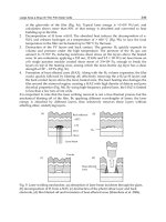
2.2.1 System model
A typical system model for downlink CoMP joint transmission is described in Fig. 3. In the
system, cell users are divided into two classes, namely cell-centre users (CCUs) and cell-

edge users (CEUs). We assume only CEUs can be configured to work under CoMP mode.
Each CEU has a CoMP Cooperating Set (CCS) formed by the cells that provide data
transmission service to this CEU, and the serving cell of each CUE is always included in its
CCS. The CEU with more than one cell in its CCS is regarded as a CoMP CEU, which can be
served by the cells contained in its CCS simultaneously with the same frequency resources.
It is assumed that each cell is configured with one transmitting antenna with one receiving
antenna for each user.
As shown in Fig. 3, Cell 1, Cell 2 and Cell3 are formed a CCS for user 1. So user 1 is regarded
as a CoMP CEU, and can be served by all these three cells simultaneously with the same
frequency resources. Since user 2 is not work under CoMP mode, it can only communicate
with its serving cell, i.e. Cell 1.

Cell2
Cell3
Cell1
User 2
User 1
Signal from serving cell
Signal from cooperative cell

Fig. 3. System Model for downlink CoMP joint transmission
Let
k
Ψ denote the CCS of the
th
k CoMP CEU, Ω denote the overall cells in the system, and
{
}
k
ΩΨ∩ denote the cells in set

Ω
while not in set
k
Ψ
. Therefore, the signal to interference
plus noise ratio (SINR) on
th
l physical resource block (PRB) for
th
k active CoMP CEU
connected to
th
i cell is determined as follows:

{}
k
kk
sl s sl
k
s
il
k
nl nl n
n
PG h
NxPG
2
,,
,
0,,

γ
∈Ψ
∈Ω Ψ
=
+
∑
∑
∩
(7)
Where
sl
P
,
is the transmission power from
th
s cell on
th
l PRB. For simplicity,
sl
P
,
is constant
assuming no power control.
k
s
G is the long term gain between
th
s cell and the
th
k CoMP CEU,

consisting of propagation path loss and the shadow fading.
k
sl
h
,
denotes the fast fad gain on
Advances in Vehicular Networking Technologies

362
th
l
PRB for the channel between
th
s
cell and
th
k
CoMP UE. N
0
is the noise power received
within each PRB. And
nl
x
,
is the allocation indicator of
th
l
PRB, which can be given by:

th th

nl
i
f
l PRB is used in n cell
x
otherwise
,
1,
0,
⎧
⎪
=
⎨
⎪
⎩
(8)
In 3GPP LTE standards, it was pointed out that interference coordination is handled by the
system once every 100ms. The information reported by the users and used by the system is
the average SINR value. Thus,
k
sl
h
2
,
is replaced by its mean value
(
)
k
sl
Eh

2
,
1
=
, and Eq. (7)
can be expressed as

{}
k
k
k
sl s
s
k
il
k
nl nl n
n
PG
NxPG
,
,
0,,
γ
∈Ψ
∈Ω Ψ
=
+
∑
∑

∩
(9)
For the users who don’t work under CoMP mode, they only communicate with their serving
cells. The average SINR on
th
l PRB for
th
k user of
th
i cell is then given by:

k
il i
k
il
k
nl nl n
nni
PG
NxPG
,
,
0,,
,
γ
∈Ω ≠
=
+
∑
(10)

Finally, according to Shannon theorem, the corresponding capacity to the user average SINR
on
th
l PRB can be expressed as:

k
il
k
il
CB
,
,2
log 1
γ
⎛⎞
=+
⎜⎟
⎜⎟
Γ
⎝⎠
(11)
Where
B is the bandwidth of each PRB, and
Γ
called SINR gap is a constant related to the
target BER, with
(
)
BERln 5 /1.5Γ=−
.

2.2.2 Cooperative frequency reuse scheme
The principle of the CFR scheme that can support CoMP joint transmission will be
introduced here. Each three neighbouring cells are formed as a cell cluster and respectively
marked with cell 1, cell 2 and cell 3. The cell-edge area of each cell is then divided into six
cell-edge zones according to the six different neighbouring cells. Given the marker of each
neighbouring cell, the six cell-edge zones in a cell are then categorized into two types.
Hence, there are total six types of cell-edge zones in a cell cluster. As illustrated in Fig.4,
each cell-edge zone is marked with
j
i
A , where i denotes the cell to which the zone belongs,
j
is the marker of the dominant interference cell of this zone, note that
{
}
ij, 1,2,3=
and
ij≠
. For simplifying expression, we just take the cell-edge zones in cell 1 into count:
Zone A
2
1
: It is the cell-edge zone of the cells marked with cell 1. Moreover, the dominant
interferer of the users in this zone is the nearest neighbouring cell marked with cell 2.
Zone A
3
1
: It belongs to the cells marked with cell 1. And the dominant interferer is the
nearest neighbouring cell marked with cell 3.
Inter-cell Interference Mitigation for Mobile Communication System

363
3
2
A
2
1
A
3
2
A
3
2
A
1
3
A
1
3
A
3
2
A
3
2
A
3
2
A
1

2
A
1
2
A
1
2
A
2
1
A
2
1
A
3
1
A
3
1
A
3
1
A
1
3
A
Cell1
Cell 2
Cell 2
Cell 2

Cell 3 Cell 3
Cell 3

Fig. 4. Cell-edge areas partition for each cell
In order to support multi-cell joint transmission with neighbouring cells, a cooperative
frequency subset is defined for each cell in CFR scheme. Then the resources are allocated to
users in each cell cluster according to the following frequency reuse rule:
Step1. In each cell, the whole resources are divided into two sets, G and
F , where GF=∅∩ .
Resources in set G are used for CCUs in each cell. While resources in set F are used for
CEUs.
Step2. Set F is further divided into three subsets, marked by FFF
123
,,, with
(
)
ij
FF i
j
=∅ ≠∩
.
Step3. For each cell cluster,
i
F is assigned for cell i as a cooperative frequency subset, which
is used for providing cooperative data transmission for the CEUs in neighbouring cells.
Step4.
j
F is assigned for the CEUs in cell-edge zones marked with
j
i

A .
Based on the above mentioned frequency reuse rule, the frequency allocation for a cell
cluster is shown in Fig. 5.

3
2
A
1
3
A
1
3
A
3
1
A
3
2
A
2
1
A
2
1
A
2
1
A
1
2

A
3
2
A
1
2
A
3
1
A
1
2
A
3
2
A
3
1
A
3
2
A
1
3
A
3
2
A
1
F

2
F
3
F
Cell 3
Cell 2
Cell1
G

Fig. 5. Frequency assignment for the boundary areas of each cell cluster
On the one hand, orthogonal frequency subsets are allocated to the adjacent cell-edge zones
that belong to different cells. Hence, the ICI can be reduced by using different frequency
Advances in Vehicular Networking Technologies

364
resources in adjacent areas of neighbouring cells. On the other hand, according to the
frequency reuse rule,
j
F is allocated for cell-edge zone
j
i
A . Besides, it is the cooperative
frequency subset for cell j , which is the dominant interference cell of zone
j
i
A . Hence, for a
CoMP CEU located in zone
j
i
A , cell i and cell j can form a CCS. And then provide CoMP

joint transmission for this CEU simultaneously with the same frequency resources selected
from
j
F .

1
CF
2
CF
3
CF
CEU2
CUE3
CEU1
Cell 3
Cell2
Cell1
Signal to CEU3
Signal to CEU1
Signal to CEU2

Fig. 6. CoMP joint transmission in CFR system
As shown in Fig.6, when CEU 1 in zone
A
3
1
is regarded as a CoMP CEU, its dominant
interference cell marked with cell 3 and the serving cell marked with cell 1 can form a CCS.
Then CEU 1 can be served by these two cells with the same frequency resources selected
from set F

3
. What’s more, we can see that the whole frequency resources could be reused in
all cells. Hence, the frequency reuse factor in CFR scheme can achieve to 1. In CCS selection,
we introduce an algorithm for the CCS selection. Let N denote the total number of cells in
the system,
M
denote the maximum number of cells in a CCS of a CEU. The
th
k CEU’s
CCS, denoted as
k
Ψ
, can then be selected according to the user’s long term gain
i
k
G as
follows:

Algorithm: CCS Selection
c
k
Ψ
←∅, count 0
←
.
d Calculate the long term gain
i
k
G between
th

k
CEU and
th
i
cell, for iN0, , 1
=
− .
{
}
N
kk k
GGGG
01 1
, , ,
−
←
e Find serving cell for
th
k CEU
(
)
ii
kk
iGGGarg max ,
←
∈
si
←

f Update

{
}
th
kk
icellΨ←Ψ∪
count count 1
←
+
Inter-cell Interference Mitigation for Mobile Communication System

365
g If count M
<
,
{
}
i
k
GGG←−
(
)
ii
kk
iGGGarg max ,
←
∈
Else stop.
h If
si
kk

GGthr−≤ , go to f
Else stop.

It has been proved that the maximum size of UE-specific CoMP cooperating set equal to 2 is
enough to achieve CoMP gain for 3GPP case 1 in references. Hence, the value of
M
is set to
2 in this paper. CEUs with two cells in their CCS are regarded as CoMP CEUs, whose SINR
can be improved by CoMP joint transmission with the same frequency resources according
to the introduced frequency reuse rule.
2.2.3 Performance analysis
System level simulations are performed to evaluate the performance of the introduced CFR
scheme. As performance metrics, we used the blocking probability and the average
throughput in both the cell-edge and cell-average points of view. The universal frequency
reuse (UFR) where PRBs are randomly assigned to the different users in each cell
irrespective of their category (CEU or CCU) is taken as a reference scheme. Another
reference scheme is SFR scheme, which assigns a fixed non-overlapping cell edge
bandwidth to a cluster of three adjacent cells. For the introduced CFR scheme, two cases are
studied, where
Thr is 0 dB and 5 dB respectively.
We focus on an OFDMA-based downlink cellular system. A number of UEs are uniformly
dropped within each cell. The basic resource element considered in the system is the PRB,
which consist of 12 contiguous subcarriers. It is assumed that all the available PRBs are
transmitted with equivalent power. Only one PRB can be assigned to each active UE. The
main simulation parameters listed in Table.1 are based on 3GPP standards.

Parameters Values
Carrier Frequency 2 GHz
Bandwidth 10 MHz
Subcarrier spacing 15 kHz

Number of subcarriers 600
Number of PRBs 50
The number of cells 21
Cell radius 500m
Maximum power in BS 46 dBm
Distance-dependent path loss
L=128.1+37.6log10 d (dB), d in km
Shadowing factor variance 8dB
Shadowing correlation
distance
50m
Inter cell shadow correlation 0.5
Table 1. Simulation Parameters
Advances in Vehicular Networking Technologies

366
Fig. 7 shows the blocking probability of the introduced CFR scheme and the conventional
SFR scheme as a function of the loading factor. We can see that CFR scheme performs quite
better than the SFR scheme. Specially, the blocking probability reduced by SFR scheme is
50% more than SFR scheme. For example, if it is required that the blocking probability must
not exceed 5%, Fig.7 indicates that the admissible loading factor of the SFR scheme is only
30%, while the admissible loading factor of the introduced CFR scheme is more than 60% of
the total frequency resource. This improvement in the CFR scheme results from the
frequency reuse rule designed for each cell cluster. According to the frequency reuse rule,
the number of available frequency resources for the cell-edge areas of each cell is twice as
great as the conventional SFR scheme.

0 0.1 0.2 0.3 0.4 0.5 0.6 0.7 0.8
0
0.05

0.1
0.15
0.2
0.25
Loading factor
Blocking prabability


SFR
CFR thr=5dB
CFR thr=0dB

Fig. 7. Blocking probability as a function of the loading factor
Fig. 8 shows the cell-edge average throughput per user for the three different frequency
reuse schemes considered in this paper. It can be seen that the average throughput per
CEU decreases as the number of users increases in all the three schemes. That is because
the probability of PRBs collision increases as the number of users grows. In other words,
the ICI increases when the average number of users per cell grows. Moreover, compared
with UFR scheme, both CFR scheme and SFR scheme yield a significant improvement in
terms of cell-edge average throughput owing to the frequency reuse plans for cell-edge
areas.
We can also observe that the introduced CFR scheme achieves higher cell-edge average
throughput than SFR scheme. When Thr is 0 dB, no user works under CoMP mode.
Compared with SFR scheme, the cell-edge average throughput is improved by 4 to 8%,
which is achieved mainly owing to the frequency reuse rule designed in CFR scheme. When
Thr is set to 5dB, the throughput raised by the introduced CFR scheme is 30 to 40% more
than the SFR scheme, that is because part of the CEUs are regarded as CoMP users whose
throughput can be further improved by CoMP joint transmission.
Inter-cell Interference Mitigation for Mobile Communication System

367
5 10 15 20 25 30
100
200
300
400
500
600
700
800
900
1000
Number of users
p
er cell
Cell-edge average throughput per user [Kbps]


UFR
SFR
CFR Thr=0dB
CFR Thr=5dB

Fig. 8. Cell-edge average throughput per user

5 10 15 20 25 30
5
10
15
20

Number of users per cell
Cell-average throughput [Mbps]


UFR
SFR
CFR Thr=0dB
CFR Thr=5dB

Fig. 9. Cell-average throughput as a function of the number of users per cell
Advances in Vehicular Networking Technologies

368
Fig. 9 shows the cell-average throughput of the introduced CFR scheme and the two
conventional frequency reuse schemes as a function of the number of users per cell. From
the graph, we can see that the cell-average throughput of the introduced CFR scheme
outperforms that of the SFR scheme due to better cell-edge performance and lower blocking
probability. When Thr is set to 0dB, the cell-average throughput is improved by 1 to 3%.
While when Thr is set to 5dB, the cell-average throughput is improved by 5 to 9%.
It is also can be seen that when the number of users per cell is small, i.e. less than 15, CFR
scheme with Thr equals to 5dB achieves the best results among the three schemes under
consideration. When the number of users is large, UFR scheme achieves the better results
than the introduced CFR scheme. However, the payoff for this higher average cell
throughput of UFR scheme is a huge decrease in cell-edge average throughput which can be
observed from Fig. 8.
2.2.4 Summary
In this part, a novel frequency reuse scheme named CFR is introduced to support CoMP
joint transmission and further improve cell-edge performance. First, the method for cell-
edge areas partition is introduced, which divides the cell-edge areas of each cell into two
types of zones. Then, the frequency plan rule is defined for each cell cluster, which assigns a

cooperative frequency subset for each cell and makes CoMP users in cell-edge zones can be
served by multi-cell joint transmission with the same frequency resources. In addition, the
algorithm is given for the CEUs to select cells in their CCS. The simulation results
demonstrate that the introduced CFR scheme significantly outperforms the conventional
SFR scheme in terms of blocking probability, cell-edge average throughput and cell-average
throughputs.
3. Inter-cell interference prediction
In order to mitigate the inter-cell interference in OFDMA systems, three schemes are given
in 3GPP organization, which respectively are interference coordination, interference
cancellation and interference randomization. However, the traditional inter-cell interference
mitigation schemes belong to passive interference suppression measures, and its
effectiveness is still limited. Considering this situation, an active interference mitigation
strategy will be introduced in this part, named as interference prediction. By means of the
immediate interference prediction in cell, it enables to efficiently avoid and eliminate inter-
cell interference, which is a novel type of active interference mitigation strategy.
For interference prediction, this part takes use of the optimal estimation theory. Generally,
the problems about optimal estimation theory can be classified into three categories: The
first is the model parameter estimation problem, such as the least squares method. The
second is time series and optimal filtering estimates problem (the optimal estimation of
signal or state). The third is the optimal information fusion estimation. According to the
actual situation in inter-cell interference prediction, the second problem of optimal
estimation is focused.
The inter-cell interference prediction principle is based on optimal estimation theory,
forecasting the co-frequency interference in the next timeslot by means of the former or
current channel state, and making the mean square error to be the smallest. The optimal
estimation theory includes time-series estimation, optimal filtering estimation method, etc.
Inter-cell Interference Mitigation for Mobile Communication System

369
Especially, the optimal filtering estimation aims to estimate the signal state, including

several filtering estimation algorithms, such as Wiener filter, Kalman filter, and so on.
3.1 Time series
In time series analysis, it aims to establish the time series model, predict and control signal
change state based on such model. Moreover, we define the observation sequence as
{
}
tn
zz z z
12
,,,,, the linear mixed coefficient as
{
}
tn
aa a a
12
,,,,, then the future
value
{
}
tk
zk0
+
> can be predicted by means of current and past time series records
{
}
tt t
zz z
12
,,,
−−


. The predicted value is written as
tkt
z
ˆ
+
, which meets following condition:

iti
tkt
i
zaz
0
ˆ
∞
−
+
=
=
∑
(12)
The optimal predicted value
tkt
z
ˆ
+
should make the mean square error be minimum, which
should obey

()

tk
tkt
Min E z z
2
ˆ
+
+
⎧
⎫
⎡
⎤
−
⎨
⎬
⎢
⎥
⎣
⎦
⎩⎭
(13)
In the above theoretical derivation, the present and past observed records
{
}
tt t
zz z
12
,,,
−−
 belong to be infinite series, which is difficult to achieve in practice.
Considering this situation, the finite time series of recursive predictor are introduced, such

as Box-Jenkins method, Astrom method, etc. Besides, the steps of Box-Jenkins method are as
follows:
a. For the observed sequence
{
}
t
zt N1,2, ,=  , calculate its correlation coefficient and
partial autocorrelation coefficient, then test whether the sequence is non-stationary
white noise sequence. If such sequence is white noise series, go to the end. If such
sequence is non-stationary series, take model according to non-stationary time series
principle. Else if the sequence is stationary series, take zero for the mean of such
sequence and then make model by the Box-Jenkins method.
b. Test the type of zero mean stationary series. Illustrately, determine the series
{
}
t
zt N1,2, ,=  belong to which model, such as autoregressive (AR) model, moving
average (MA) model and autoregressive moving average (ARMA) model.
c. After the model is identified, judge the highest level of such model, and make fitted test
from low level to high level. For example, if
{
}
t
zt N1,2, ,=  belong to AR model, make
use of
(
)
AR n n,1
−
, and then the fitted test.

d. Compare with different models and find the right model. On this basis, respectively
take adaptive test and error test for the initial model, and select the optimal model.
e. Make prediction by the established model.
3.2 Optimal filter estimation
The nature of filtering is the statistical estimation problem. For example, linear minimum
variance estimation methods try to make the variance of estimated value and the actual
value minimum. Moreover, such filter is also known as the optimal filter, such as Wiener
filter and Kalman filter. The interference prediction process by Kalman filter is shown
respectively in Fig. 10 and Fig. 11.
Advances in Vehicular Networking Technologies

370
Initial ,
Calculate interference in prior
Calculate covariance in prior
Calculate Kalman factor
Calculate the revised interference value
Calculate the revised covariance
1kk
=
+
ˆ
(1/ 1)Xk k
−
−
(1/1)Pk k
−
−
ˆ
ˆ

(/ 1) ( 1/ 1)Xk k Xk k
−
=Φ − −
(/ 1) ( 1/ 1)
T
Pk k Pk k Q
−
=Φ − − Φ +
1
() (/ 1) [ (/ 1) ]
TT
Kk Pk k H HPk k H R
−
=− −+
ˆ
ˆˆ
(/) (/ 1) ()[() (/ 1)]Xkk Xkk KkZk HXkk
=
−+ − −
(/) [ () ](/ 1)Pk k I KkHPk k
=
−−
1kk
=
+
Estimate the interference
in next time
ˆ
ˆ
(1/) (/)

X
kk Xkk+=Φ

Fig. 10. Interference prediction by Kalman filter


Fig. 11. Interference prediction results by Kalman filter
3.3 Effectiveness principles
The effectiveness of channel prediction criteria was analyzed and the relationship with the
predicted time delay and the prediction accuracy of SINR are described in the reference.
According to the wireless signal propagation, the mobility rate is closely related with the
signal coherence time. If user’s mobility rate increases, the coherence time becomes shorter.
0 20 40 60 80 100 120 140 160 180 200
-8
-6
-4
-2
0
2
4
6
8
10
time(s)
signal strength(dBm)
Estimated Signal (k+1)
Interference Signal
Inter-cell Interference Mitigation for Mobile Communication System

371

Else user’s mobility rate decreases, the coherence time becomes longer. The relationship of
coherence time and the predicted delay time are divided into three categories,
respectively t
τ
Δ , t
τ
≅
Δ and t
τ
Δ
 .
Fig.12 shows the prediction results when the coherence time is much greater than the time
delay, which is that t
τ
Δ
 . At this time, user is in a slow moving state, and the channel
state information (CSI) can be easily obtained. From Fig.12, we can see the predicted SINR in
delay time approximates to the actual value.

SINR
Predicted value
delay t

Fig. 12. SINR prediction (
t
τ
Δ
 )
Fig.13 shows the prediction results when the coherence time approaches to the time delay,
which is that

t
τ
≅Δ . At this time, user’s moving speed is in a medium state. In order to
ensure the continuity of information transmission, the SINR should obey the outage criteria
and keep a conservative prediction, which is the threshold SINR value.


SINR
conservative predicted value
delay
t

Fig. 13. SINR prediction ( t
τ
≅
Δ )
Advances in Vehicular Networking Technologies

372
Fig. 14 shows the prediction results when the coherence time is far less than the time delay,
which is that t
τ
Δ
 . At this time, user’s rate is in a high speed state, the coherence time is
shorter and the CSI is hard to be obtained. In this situation, we only need to predict the
average SINR.


SINR
Predicted value

delay
t

Fig. 14. SINR prediction ( t
τ
Δ
 )
3.4 Summary
In this part, the inter-cell interference prediction is introduced, which is an active
interference mitigation method. The theoretical basis, which is the optimal estimation
theory, is provided with including of two parts: time series and the optimal filter estimation.
Besides, the reliability is also analyzed by means of prediction accuracy, which is based on
the relationship of the coherent time and the time delay. In addition, the trend for the actual
measured radio signals is analyzed with AR model, MA model and ARIMA model. The
analytical results are provided to show time series model can efficiently predict the radio
signals change and then mitigate the interference effectively.
4. Inter-cell interference cancellation
Inter-cell interference cancellation strategy aims at interference suppression at the user
equipments by improving the processing gain. In order to solve this problem, two basic
schemes have been discussed in 3GPP proposals. One is to take spatial suppression at the
UE side by means of multiple antennas; the other is to directly detect and subtract the inter-
cell interference in order to enable inter-cell-interference cancellation. Usually, the inter-cell
interference cancellation strategy is used to get the processing gain through suppress strong
interference. According to the degree of knowledge available about interferers, interference
cancellation methods can be distinguished as three categories, which are blind, semi-blind,
and full-knowledge.
Many inter-cell interference cancellation methods are based on generalized spatial diversity.
Beam forming is introduced in inter-cell interference cancellation in references. By
distinguish different users in space, it effectively reduces interference among users. But on
Inter-cell Interference Mitigation for Mobile Communication System

373
the other hand, it brings with extra interference from main lobe and strong side lobe. A
method of subcarrier-based virtual MIMO in inter-cell interference cancellation was
proposed, which is introduced in OFDM-based systems with a frequency reuse factor equal
to 1. But when UE is located between sectors, inter-sector interference cannot be reduced by
the subcarrier-based virtual MIMO (SV-MIMO) due to loss of channel separability. Inter-cell
interference cancellation by virtual smart antennas was also studied, which proposes a
method for estimating inter-cell symbol timing offsets using multiple signal classification
(MUSIC) algorithm. For the use of MUSIC algorithm, the premise is to know the number of
source. But in practice, the number of source can not be accurately obtained, which may
make MUSIC algorithm not work. Moreover, in most case, many similar algorithm needs to
know current channel state information, but at the same time, the complexity of system may
be increased if acquire it in downlink. As a result, how to mitigate inter-cell interference in
no precise channel is an important problem.
In order to effectively mitigate inter-cell interference in OFDM-based systems, this part
focuses on the inter-cell interference cancellation strategy. A novel inter-cell interference
mitigation method for OFDM-based cellular systems will be introduced. Compared to the
existing methods, the independent component analysis based on blind source separation is
presented in inter-cell interference, and the signal to interference plus noise (SINR) is set up
as the objective function. This scheme can adapt to the no precise channel conditions, and
can mitigate inter-cell interference in a semi-blind state of source signal and channel
information.
4.1 Inter-cell interference model
Considering the downlink in cell-edge, assume this MIMO system with
q
transmission
antennas in the serving eNodeB, and
p
receiving antennas in UE. In such scenario, UE not

only receives useful signal from current communicating base station, but also receives noise
and interference from other adjacent base stations. The example is shown in Fig. 15.


BS
eNode B1
eNode B 3
UE
eNode B 2

Fig. 15. Inter-cell interference in cell-edge
For many OFDM-based systems, the original signal is transmitted from OFDM transmitter
and through MIMO antenna array. The process of inter-cell interference mitigation is shown
in Fig.16. Further, we assume the original signal interfered by inter-cell interference and
thermal noise, and the channel information is unknown.
Advances in Vehicular Networking Technologies

374

.
.
.
MIMO System
OFDM
Transmitter
.
.
.
OFDM
Transmitter

.
.
.
OFDM
Receiver
OFDM
Receiver
.
.
.
Whitening
ICA algorithm
.
.
.
y(t)=Wx(t) P/S
.
.
.
Remove
means
r1(t)
x1(t )
Whitening
Remove
means
rp(t)
xp(t)
.
.

.
Inter-cell Interference Cancellation
Inter-cell interfernc e i(t)
thermal noise n(t)

Fig. 16. Inter-cell interference mitigation process
According to the principle in radio signal propagation, the thermal noise can be seen as
independent with transmission signals from eNodeB. Compared to the inter-cell
interference from other cells, we assume the useful signal is statistically independent with
the co-frequency interference from other different cells. So it can be thought that useful
signal, unknown inter-cell interference and thermal noises are statistically independent and
irrelevant with each other. Moreover, some parameters are defined as follows:
kn
st ut i t i t i t nt
12
( ) { ( ), ( ), , ( ), , ( ), ( )}
−
= denotes as the source signal, which is constructed by
the useful signal, inter-cell interference and the thermal noise, also written as
T
n
ss s
12
(,, ,).
Specifically,
ut()denotes as the useful signal.
k
it() denotes as the kth unknown additive
inter-cell interference with the same frequency, which is in the range of 1 to n 2− . The
dimension for the number of eNodeB reused with the co-frequency subcarriers is n 2− .

nt() denotes as the additive zero mean thermal noise, also the Gaussian noise.
At the receiving end, we denote
rt() as the received signal, mixed with the useful signal,
unknown additive interference and noise.
k
,
α
β
and
γ
are respectively the mixing vectors.
So
rt()can be written as the following equation:

n
kk
k
rt ut i t nt
2
1
() () () ()
αβγ
−
=
=+ +
∑
(14)
Furthermore, Let
A
denote as linear mixing matrix, which reflects temporal radio signals

transmission process and all interference from other adjacent cells are linear mixture. Then
the inter-cell interference model can be written as:

rt Ast() ()=
(15)
From Eq.(15), it can been seen that the dimension of
rt()is the same to st(), which is equal
to
n . In order to separate the useful signal from inter-cell interference and thermal noise, we
take interference cancellation by independent component analysis (ICA), which is an
important method in blind source separation (BSS). As shown in Fig.16, we deal with the
received signal by remove means and whitening, and such process is set as the transition
matrix
V . So we can get:

xt Vrt() ()
=
(16)
Inter-cell Interference Mitigation for Mobile Communication System

375
On the other side, we set up a separation matrix W , and make WVA I= in theory.
Moreover, assume
y
t()is the separated signal after removing interference and noise,
so
yt()
can be got by following equation:

y

tWxtWVAstGst() () () ()
=
== (17)
But in fact, because exist with errors and uncertainties, we need to get an optimal
approximate solution that can make such a separation matrix
W approach to the
condition
GI= . By means of ICA methods, an objective function is established, which takes
W as a variable function. When W takes some value, the objective function can achieve to
minimum or maximum. At this moment, the variable
W is the optimal approximate
solution.
4.2 Independent component analysis
In many fields, it needs to separate all the source signals from the mixed signals with no
precise knowledge of the source signals and the channel information, whose processes are
usually called as blind source separation (BSS). In order to solve such problem, many
schemes have been researched. When the source signals are not independent with each other
in BSS, some separating schemes are introduced, such as sparse component analysis (SCA),
smooth component analysis (SMOCA), non-negative matrix factorization (NMF), and so on.
However, the complexity of such algorithms is still high and hard to realize in application.
On the other hand, when the source signals are independent with each other in BSS, the
independent component analysis (ICA) schemes are proposed. By principle of
independence, the separating complexity is reduced and the results are also improved.
Specially, some methods exist in ICA, such as Informax, Fast ICA, generalized eigenvalue
decomposition, etc. Informax algorithm is proposed by Bell, whose characteristic is
searching for the maximum mutual information between the received signal and the output
signal, but its convergence is always slowly. Fast ICA is a fast and fixed-point algorithm
proposed by A. Hyvrinen, whose characteristic is computing the maximum kurtosis by
iterations. Although its convergence is improved compared with Informax, the effects of
thermal noise are always not included in iterations. The ICA based on generalized

eigenvalue decomposition is proposed by L. Parra, whose characteristic is decomposing
generalized eigenvalue for the received signal. However, this method is limited by the type
of source signals.
The critical step in ICA process is to make the estimated independent component gradually
approach to the source signal by means of establishing objective function and finding its
optimal solution.
According to the classical formula dealing with ICA problems, some requirements must be
made in the known conditions in order to get definite solution, as follows:
a. The source signals are all real random signals, and the respective mean is zero.
Moreover, these signals are statistically independent with each other.
b. There is at most one source signal whose probability density characteristic is the
Gaussian distribution, while the other source signals obey non-Gaussian probability
distribution.
c. For the source signals, the approximate probability distribution functions (PDF) need to
be acquired.