Artificial Neural Networks Industrial and Control Engineering Applications Part 13 ppt

System Identification of NN-based Model Reference Control of RUAV during Hover

409

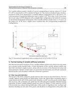
Fig. 12. Transfer function of system
5. Experimental results and analysis
In this experiment we used NN approach to train MIMO model and capture the phenomena
of flight dynamics. This simulation is divided into two parts longitudinal mode and Lateral
mode. The NN approach considers separate lateral and longitudinal network with inertial
coupling between the networks taken into consideration. These networks trained
individually by making it MIMO model. Basically system identification process consists of
gathering experimental data, estimate model from data and validate model with
independent data. NN controller is designed in such a way that makes the plant output to
follow the output of a reference model. The main target is to play with fine tuning of
controller in order to minimize the state error.
The experiment is carried out with System identification procedures with Prediction Error
Method (PEM) algorithm using System Identification Toolbox using Levenberg-Marquardt
(LM) algorithm. We observe NN approach to get better result of System identification that
shows the perfect matching and shown as RUAV Longitudinal Dynamics and RUAV Lateral
Dynamics in the following fig. 13-18
The prediction error of the output responses is described in Fig. 14. The autocorrelation
function almost tend to zero and the cross correlation function vary in the range of -0.1to 0.1.
This shows the dependency between prediction error and
coll
δ
,
lon
g
δ
but the dependency
rate is very less.

Artificial Neural Networks - Industrial and Control Engineering Applications

410
Longitudinal Dynamics Mode Analysis


(a) Pitch Angle (
θ
)

(b) Forward Velocity (u)

(c) Vertical velocity (w)
System Identification of NN-based Model Reference Control of RUAV during Hover

411



(d) Pitch Angular Rate (q)

Fig. 13. Output response with network response in Longitudinal dynamics mode




(a) Pitch Angle (
θ
)
Artificial Neural Networks - Industrial and Control Engineering Applications

412

(b) Forward velocity (u)

(c) Vertical velocity (w)
System Identification of NN-based Model Reference Control of RUAV during Hover

413



(d) Pitch Angular Rate (q)

Fig. 14. Autocorrelation and Cross-correlation of output response in longitudinal mode
The histogram of prediction error is shown in Fig. 15.





Fig. 15. Histogram of Prediction errors in Longitudinal Mode
Artificial Neural Networks - Industrial and Control Engineering Applications

414
Lateral Dynamics Mode Analysis


(a) Roll Angle (
ϕ

)

(b) Lateral Velocity (v)


(c) Roll Angular Rate (P)
System Identification of NN-based Model Reference Control of RUAV during Hover

415

(d) Yaw Angular Rate (r)
Fig. 16. Output response with network response in lateral dynamics mode
The prediction error of the output responses is described in Fig. 17. Similarly, in lateral
mode also, the autocorrelation function almost tend to zero and the cross correlation
function vary in the range of -0.1to 0.1. This shows the dependency between prediction error
and
lat
δ
,
p
ed
δ
but the dependency rate is very less.




(a) Roll Angle (
ϕ
)

Artificial Neural Networks - Industrial and Control Engineering Applications

416

(b) Lateral Velocity (v)

(c) Roll Angular Rate (P)
System Identification of NN-based Model Reference Control of RUAV during Hover

417

(d) Yaw Angular Rate (r)
Fig. 17. Autocorrelation and Cross-correlation of output response in lateral mode
The histogram of prediction error is shown in Fig. 18.
6. Conclusion
UAV control system is a huge and complex system, and to design and test a UAV control
system is time-cost and money-cost. This chapter considered the simulation of identification
of a nonlinear system dynamics using artificial neural networks approach. This experiment
develops a neural network model of the plant that we want to control. In the control design
stage, experiment uses the neural network plant model to design (or train) the controller.
We used Matlab to train the network and simulate the behavior.
This chapter provides the mathematical overview of MRC technique and neural network
architecture to simulate nonlinear identification of UAV systems. MRC provides a direct
and effective method to control a complex system without an equation-driven model. NN
approach provides a good framework to implement MEC by identifying complicated
models and training a controller for it.
7. Acknowledgment
“This research was supported by the MKE (Ministry of Knowledge and Economy), Korea,
under the ITRC (Information Technology Research Center) support program supervised by
the NIPA (National IT Industry Promotion Agency)” (NIPA-2010-C1090-1031-00003)

Artificial Neural Networks - Industrial and Control Engineering Applications

418


Fig. 18. Histogram of Prediction errors in Longitudinal Mode
8. References
[1] A. U. Levin, k. s Narendra,” Control of Nonlinear Dynamical Systems Using Neural
Networks: Controllability and Stabilization”,
IEEE Transactions on Neural Networks,
1993, Vol. 4, pp.192-206
[2] A. U. Levin, k. s Narendra,” Control of Nonlinear Dynamical Systems Using Neural
Networks- Part II: Observability, Identification and Control”,
IEEE Transactions on
Neural Networks
, 1996, Vol. 7, pp. 30-42
[3] David E. Rumelhart et al., “The basic ideas in neural networks”, Communications of the
ACM, v.37 n.3, p.87-92, March 1994
[4] E. R. Mueller, "Hardware-in-the-loop Simulation Design for Evaluation of Unmanned
Aerial Vehicle Control Systems",
AIAA Modeling and Simulation Technologies
Conference and Exhibit ,
20 - 23 August, 2007, Hilton Head, South Carolina
[5] E. N. Johnson and S. Fontaine, "Use of flight simulation to complement flight testing of
low-cost UAVs",
AIAA Modeling and Simulation Technologies Conference and Exhibit,
Montreal, Canada, 2001
[6] MATLAB and Simulink for Technical Computing, Available from:

[7] Oliver Nelles, "Nonlinear System Identification: From Classical Approaches to Neural

Networks and Fuzzy Models, Springer
System Identification of NN-based Model Reference Control of RUAV during Hover

419
[8] Cybenko, G., “Approximation by Superposition of a Sigmoidal Function, Mathematics of
Control, Signals and Systems, 303-314.
[9] N. K. and K. Parthasarathy, Gradient methods for the optimization of dynamical systems
containing neural networks.
IEEE Trans. on Neural Networks, 252-262.
[10] B.G Martzios and F.L. Lewis, “An algorithm for the computation of the transfer
function matrix of generalized two-dimensional systems ”
Journal of Circuit, System,
and Signal Processing
, Volume 7, Number 4 / December, 1988
[11] Budiyono A, Sudiyanto T, Lesmana H., “First Principle Approach to Modelling of
Small Scale Helicopter”, International Conference on Intelligent Unmanned System,
2007
[12] B. Mettler, T. Kanade, M.B. Tischler, "System Identification Modeling of a Model-Scale
Helicopter", CMU-RI-TR-00-03. 2000.
[13] E. D. Beckmann, G. A. Borges, "Nonlinear Modeling, Identification and Control for a
Simulated Miniature Helicopter," Robotic Symposium. LARS’08, pp.53-58, 2008.
[14] D. W. Marquardt. “An algorithm for least-squares estimation of nonlinear parameters”.
SIAM Journal on Applied Mathematics, Vol. 11 No.2 pp. 431–441, 1963.
[15] S. Haykin, “Neural networks: A comprehensive foundation”, IEEE Press, New York,
USA, 1994
[16] K. S. Narendra and K. Parthasarathy, “Identification and control of dynamical systems
using neural networks,” IEEE Transactions on Neural Networks, vol. 1, no. 1, pp.
4–27, 1990.
[17] La Civita, M., G., P., Messner, W. C., and Kanade, T., “Design and Flight Testing of a
High-Bandwidth H∞ Loop Shaping Controller for a Robotic Helicopter,”

Proceedings of the AIAA Guidance, Navigation, and Control Conference, No.
AIAA 2002-4836, 2002.
[18] Sahasrabudhe, V., & Celi, R., “Improvement of off-design characteristics in integrated
rotor-flight control system optimization”. AHS, annual forum 53rd Virginia Beach,
VA, April 29–May 1, 1997, Proceedings. Alexandria, VA, American Helicopter
Society, 1997. Vol. 1 (A97-29180 07-01).
[19] Smerlas, A., Postlethwaite, I., Walker, D. J., Strange, M. E., Howitt, J., Horton, R. I.,
Gubbels, A. W., & Baillie, S. W. , “Design and flight testing of an H-infinity
controller for the NRC Bell 205 experimental fly-by-wire helicopter. AIAA GNC
conference, 1998.
[20] Li-Xin Wang, “Design and analysis of fuzzy identifiers of nonlinear dynamic systems”.
IEEE Transactions on Automatic Control, 40(1), 1995.
[21] Shaaban A. Salman, Vishwas R. Puttige, and Sreenatha G. Anavatti, “Real-time
Validation and Comparison of Fuzzy Identification and State-space Identification
for a UAV Platform” Proceeding of the 2006 IEEE International Conference on
Control Applications, pages 2138–2143, 2006.
[22] R. Pintelon and J. Schoukens, “System Identification: A Frequency Domain Approach”
Wiley-IEEE Press, 1st edition, 2001.
[23] Kumpati S. Narendra and Kannan Parthasarathy, “Identification and Control of
Dynamical Systems Using Neural Networks” IEEE transaction on Neural
Networks, 1(1), 1990.
[24] Magnus Norgaard, “Neural Network Based System Identification Tool Box”, Version 2,
2000
Artificial Neural Networks - Industrial and Control Engineering Applications

420
[25] Budiyono, A. and Sutarto, H.Y., Linear Parameter Varying Model Identification for
Control of Rotorcraft-based UAV, Fifth Indonesia-Taiwan Workshop on
Aeronautical Science, Technology and Industry, Tainan, Taiwan, November 13-16,
2006

[26] M. M. Korjani, O.Bazzaz, M. B. Menhaj, ”Real time identification and control of
dynamics systems using recurrent neural network”, Journal of Artificial
Intelligence Review, Springer, August 2009
[27] W. Yu, X. Li, “Recurrent fuzzy neural networks for nonlinear system identification”,
22nd IEEE International Symposium on Intelligent Control Part of IEEE Multi-
conference on Systems and Control, Singapore, 1-3 October 2007.
[28] Shim D. H., Kin H. J., Sastry. “Control System Design for Rotorcraft-based Unmanned
Aerial Vehicles using Time-domain System Identification”. IEEE International
Conference on Control Application, 2000. pp. 808-813
20
Intelligent Vibration Signal Diagnostic System
Using Artificial Neural Network
Chang-Ching Lin
Tamkang University Tamshui, Taipei County,
Taiwan
1. Introduction
In today’s sophisticated manufacturing industry maintenance personnel are constantly
forced to make important, and often costly, decisions on the use of machinery. Usually,
these decisions are based on practical considerations, previous experiences, historical data
and common sense. However, the exact determination of machine conditions and accurate
prognosis of incipient failures or machine degradation are key elements in maximizing
machine availability.
The practice of maintenance includes machine condition monitoring, fault diagnostics,
reliability analysis, and maintenance planning. Traditionally, equipment reliability studies
depend heavily on statistical analysis of data from experimental life-tests or historical failure
data. Tedious data collection procedures usually make this off-line approach unrealistic and
inefficient for a fast-changing manufacturing environment (Singh & Kazzaz, 2003). Over the
past few decades technologies in machine condition monitoring and fault diagnostics have
matured. Many state-of-the-art machine condition monitoring and diagnostic technologies
allow monitoring and fault detection to perform in on-line, real-time fashion making

maintenance tasks more efficient and effective. Needless to say, new technologies often
produce new kinds of information that may not have been directly associated with the
traditional maintenance methodologies. Therefore, how to integrate this new information
into maintenance planning to take advantages of the new technologies has become a big
challenge for the research community.
From the viewpoint of maintenance planning, Condition Based Maintenance (CBM) is an
approach that uses the most cost effective methodology for the performance of machinery
maintenance. The idea is to ensure maximum operational life and minimum downtime of
machinery within predefined cost, safety and availability constraints. When machinery life
extension is a major consideration the CBM approach usually involves predictive
maintenance. In the term of predictive maintenance, a two-level approach should be
addressed: 1) need to develop a condition monitoring for machine fault detection and 2)
need to develop a diagnostic system for possible machine maintenance suggestion.
The subject of CBM is charged with developing new technologies to diagnose the machinery
problems. Different methods of fault identification have been developed and used
effectively to detect the machine faults at an early stage using different machine quantities,
such as current, voltage, speed, efficiency, temperature and vibrations. One of the principal
tools for diagnosing rotating machinery problems is the vibration analysis. Through the use
Artificial Neural Networks - Industrial and Control Engineering Applications

422
of different signal processing techniques, it is possible to obtain vital diagnostic information
from vibration profile before the equipment catastrophically fails. A problem with
diagnostic techniques is that they require constant human interpretation of the results. The
logical progression of the condition monitoring technologies is the automation of the
diagnostic process. The research has been underway for a long time to automate the
diagnostic process. Recently, artificial intelligent tools, such as expert systems, neural
network and fuzzy logic, have been widely used with the monitoring system to support the
detection and diagnostic tasks.
In this chapter, artificial neural network (ANN) technologies and analytical models have

been investigated and incorporated to present an Intelligent Diagnostic System (IDS), which
could increase the effectiveness and efficiency of traditional condition monitoring diagnostic
systems.
Several advanced vibration trending methods have been studied and used to quantify
machine operating conditions. The different aspects of vibration signal and its processing
techniques, including autoregressive (AR) parametric modeling and different vibration
trending methods are illustrated. An example of integrated IDS based on real-time, multi-
channel and neural network technologies is introduced. It involves intermittent or
continuous collection of vibration data related to the operating condition of critical machine
components, predicting its fault from a vibration symptom, and identifying the cause of the
fault. The IDS contains two major parts: the condition monitoring system (CMS) and the
diagnostic system (DS). A neural network architecture based on Adaptive Resonance
Theory (ART) is introduced. The fault diagnostic system is incorporated with ARTMAP
neural network, which is an enhanced model of the ART neural network. In this chapter, its
performance testing on simulated vibration signals is presented. An in-depth testing using
lab bearing fault signals has been implemented to validate the performance of the IDS. The
objective is to provide a new and practicable solution for CBM.
Essentially, this chapter presents an innovative method to synthesize low level information,
such as vibration signals, with high level information, like signal patterns, to form a rigorous
theoretical base for condition-based predictive maintenance.
2. Condition monitoring system
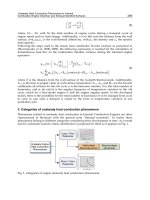
The condition monitoring system developed contains four modules (see Fig. 1): data
acquisition, Parameters Estimation (PE), Performance Monitoring (PM), and Information
Display and Control (IDC). The entire system was coded using C programming language.
We have developed a user friendly graphic interface that allows for easy access and control
in monitoring an operating machine. The system has been tested and verified on an
experimental lab setting. The detailed procedure of ISDS and programming logic is
discussed in the following sections.
2.1 Data acquisition module
The data acquisition module is more hardware related than the other modules. Vibration

signals were acquired through accelerometers connected to a DASMUX-64 multiplexer
board and a HSDAS-16 data acquisition board installed in a PC compatible computer. The
multi-channel data acquisition program controlling the hardware equipment has been
coded.
Intelligent Vibration Signal Diagnostic System Using Artificial Neural Network

423
Sensor
1
Sensor
2
Sensor
3
|
|
|
Sensor
N
Machining
Center
*
Based on the research by Hsin-Hao Huang: “Transputer-Based Machine Fault Diagnostics,” Ph. D. Dissertation,
Dept. of Industrial Engineering, The University of Iowa, Iowa City, IA, August 1993.
Condition Monitoring System
Information
Display
and
Control
Frequency
Domain

Analysis
ARPSD
FFTPSD
Parametric
Model
AR(p)
Vibration
Signal
Performance Monitoring
Channel
Selection
Data
Acquisition
Parameter Estimation
•Machine ID, Position ID
•Channel Number
•Sampling Rate
•AR Order p
•AR Parameters (Normal Condition)
•EWMA Upper Control Limit
•RMS Upper Control Limit
•Machine On/Off Threshold
Maintenance
Suggestion
Fault
Diagnostic
System
Information Flow Control Flow
Vibration
Trending

Index
EWMA
RMS
Machine
Condition
Green
Yellow
Red
ARTMAP
*
Machine
Fault
Diagnostic

Fig. 1. Overview of intelligent diagnostic system
2.2 Programming logic for Parameter Estimation (PE) module
The parameter estimation module is designed to estimate the parameters of the normal
condition of a machine. It provides a procedure to set up the machine positions considered
to be critical locations of the machine. The PE module must be executed before running the
PM module. The information to be calculated in the PM module needs to be compared to
the base-line information generated in the PE module.
The normal operating condition of a machine position is usually defined by experience or
from empirical data. Generally speaking, a particular operation mode of a machine is
selected and then defined as a “normal condition”. However, this normal condition is not
unchangeable. Any adjustment to the machine, such as overhaul or other minor repairs,
would change its internal mechanisms. In this case, the normal condition must be redefined,
and all the base-line data of the monitored positions on the machine need to be reset.
The PE procedure starts with specifying the ID of a machine, its location ID, and several other
parameters related to each position, such as channel number and sampling rate. Then the
upper control limits of the Exponentially Weighted Moving Average (EWMA) (Spoerre, 1993)

and Root Mean Square (RMS) (Monk, 1972; Wheeler 1968) vibration trending indices are
determined and an adequate Autoregressive (AR) order is computed. The AR time series
modelling method is the most popular parametric spectral estimation method which translates
a time signal into both frequency domain and parameter domain (Gersch, 1976). Once the AR
order is determined, the AR parameters can be estimated through several normal condition
signals collected from the particular position. A major issue with the parametric method is
determining the AR order for a given signal. It is usually a trade-off between resolution and
unnecessary peaks. Many criteria have been proposed as objective functions for selecting a
Artificial Neural Networks - Industrial and Control Engineering Applications

424
“good” AR model order. Akaike has developed two criteria, the Final Prediction Error (FPE)
(Akaike, 1969 ) and Akaike Information Criterion (AIC) (Akaike, 1974). The criteria presented
here may be simply used as guidelines for initial order selection, which are known to work
well for true AR signals; but may not work well with real data, depending on how well such
data set is modelled by an AR model. Therefore, both FPE and AIC have been adapted in this
research for the AR order suggestion.


Yes
N
o
Begin Parameter Estimation (PE) module
Enter machine ID, position ID, channel number, sampling rate
Initialize A/D Board
Search AR order
Acquire signals
Compute AR order using AIC, FPE criteria
Enter AR order
Yes

N
o
Acquire signals
Calculate AR parameters
Calculate EWMA-UCL, RMS-UCL, ON/OFF threshold
Close setup file
Open setup file
Start Performance Monitoring (PM) Module
Set up another position
Update setup log file


Fig. 2. Flowchart of parameter estimation (PE) module
Intelligent Vibration Signal Diagnostic System Using Artificial Neural Network

425
A setup file is then generated after the PE procedure is completed. This file, given a name
that combines the machine ID and the position ID, consists of all the parameters associated
with the specific position. The number of setup files created depends on the number of
positions to be monitored in the PM mode, that is, each monitored position is accompanied
by a setup file.
In order to perform a multi-channel monitoring scheme a setup log file is also generated.
This file contains all the names of setup files created in the PE mode. Every time a new
position is added its setup file name is appended to the setup log file. The setup log file is
very important. It not only determines the channels needing to be scanned when the PM
program is executed, it also provides the PM program with paths to locate all the necessary
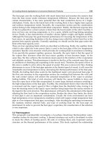
information contained in the setup files. Fig. 2 shows the programming logic of the PE
module. In practice, after the PE procedure is completed, on-line performance monitoring of
the machine (the PM mode) begins.
2.3 Programming logic for Performance Monitoring (PM) module

In the PM module, vibration data arrive through the data acquisition hardware and are
processed by AR, EWMA, ARPSD, RMS, FFT spectrum, and hourly usage calculation
subroutines. After each calculation the current result is displayed on the computer screen
through the Information Display and Control (IDC) module. Fig. 3 illustrates the flow chart
of the PM programming logic.
IDC is in charge of functions such as current information displaying, monitoring control,
and machine status reasoning. Details of these functions are given in the following section.
2.4 Information Display and Control (IDC) module
Eight separate, small windows appear on the computer screen when the IDC module is
activated. Each window is designed to show the current reading and information related to
each calculation subroutine (e.g. AR, EWMA, ARPSD, RMS, and FFT spectrum) for the
current position being monitored.
Window 1 is designed to plot the current time domain data collected from the data
acquisition equipment. Window 2 displays both the AR parameter pattern of the current
signal and the normal condition AR parameter pattern stored in the setup file generated in
the PE module. Window 3 plots the current EWMA reading on a EWMA control chart and
its upper control limit. Window 4 plots the current RMS value and its upper control limit on
a RMS control chart. Both the RMS and EWMA upper control limits are calculated in the PE
module. Window 5 displays the hourly usage and other information of the position. The
hourly usage of the position is calculated based on the vibration level of that position. It is
an estimated running time of the component up to the calculating point from the time this
position is set up. Window 6 indicates the current performance status of the position. Three
different levels of performance status: normal, abnormal, and stop, are designed. Each status
is represented by a different colour: a green light signals a normal condition; a yellow light
represents an abnormal condition; and a red light indicates an emergency stop situation.
The determination of the status of a position based on the current readings is discussed in
the next section. Window 7 gives the current ARPSD spectrum, which is calculated based on
the AR parameters from Window 2. Finally, Window 8 displays the current FFT spectrum
by using the time domain data from Window 1.
In addition to real-time information display, the IDC module also provides a user-friendly

graphic interface for monitoring control. A user can utilize the mouse to navigate around
Artificial Neural Networks - Industrial and Control Engineering Applications

426
the computer screen and click on an icon to perform the specified function. For instance, to
switch to another channel one can click on the “CH+” or “CH-” icon. Fig. 4 shows the IDC
screen layout developed.

Read in setup log file
Read in setu
p
file
Information
Display
and
Control
(IDC)
Acquire signal and plot signal in Window 1
Calculate and plot AR parameters in Window 2
Calculate and plot EWMA reading in Window 3
Calculate and plot RMS reading in Window 4
Calculate total vibration level
Vibration level
>
On/Off Threshold
Plot hourly usage and other information in Window 5
Machine in of
f
Machine is on
Update hourly usage

Calculate and plot ARPSD in Window 7
Calculate and plot FFTPSD in Window 8
EWMA > EWMA-UCL
or
RMS > RMS-UCL
Condition is normal
Condition is abnormal
Plot condition information in Window 6
Activate Fault Diagnostic System
Quit
Change
Channel
and
Other
Controls
Yes
N
o
Yes
N
o
Begin PM and IDC modules
Break

Fig. 3. Flowchart of PM and IDC modules
Intelligent Vibration Signal Diagnostic System Using Artificial Neural Network

427

Fig. 4. Condition monitoring information display and control (IDC) Screen layout
2.5 Vibration condition status reasoning
Based on the criteria stored in the setup file and the current readings, the EWMA and RMS
control charts show whether the current readings are under or above their respective upper
control limit. If both readings are under their corresponding control limits, then the position
is in a normal condition. However, if either one of the control readings exceeds its upper
control limit, the performance status reasoning program would turn on the yellow light to
indicate the abnormality of the position. In this case, the fault diagnostic system is activated.
2.6 Condition monitoring sample session
Data collection, in the form of vibration signals, was conducted using the following test rig
(see Fig. 5): a 1/2 hp DC motor connected to a shaft by a drive belt, two sleeve bearings
mounted on each end of the shaft and secured to a steel plate, an amplifier to magnify
signals, a DASMUX-64 multiplexer board, and a HSDAS-16 data acquisition board installed
in a personal computer. Vibration signals were collected from the bearing using 328C04 PCB
accelerometers mounted on the bearing housings. Using the test rig, the following sample
session was conducted.
Assume that when the motor was turned on initially, it was running in normal condition.
Later, a small piece of clay was attached to the rotational element of the test rig to generate
an imbalance condition. This was used as an abnormal condition in the experiment. In the
beginning, the setup procedure (PE) needed to be performed in order to obtain the base-li
information. The sampling rate used was 1000 Hz and the sampling time was one second.

Artificial Neural Networks - Industrial and Control Engineering Applications

428

PC
w
i
th

Da ta Acquisition Board
Moto
r
Accele
r
o
m
ete
r
Po
w
e
r
Su
p
p
lie
r
Multi
p
lexer
A
cce
l
e
r
o
m
ete
r

Moto
r
Belt
Sleeve Bea
r
i
n
g
Hu
b
Sleeve B ear
i
n
g
Acceler
o
m
eter

Fig. 5. The test rig for ISDS experiment
The PE program first acquired eight samples and then took their average. Using the average
normal signal, the AIC and FPE criteria were calculated. An AR order suggestion for the
normal condition of the test rig was made. The AR order was fixed throughout the entire
experiment. Once the AR order was known, the program started estimating the AR
parameters and upper control limits of RMS and EWMA by collecting another eight data
sets, calculating eight sets of AR parameters, and then averaging them. Finally, all
parameters were stored in the setup file which would be used in the PM stage. An example
of the normal condition parameters from a setup file are listed below:
• Machine ID: TESTRG
• Position ID: CHN1

• Channel number: 1
• Sampling rate: 1000
• AR order: 32
• AR parameters:
• EWMAUCL: 0.8912
• RMSUCL: 0.0367
When the machine was running in normal condition the readings of EWMA were
approximately -0.486 far below the EWMAUCL of 0.8912. The readings of RMS were about
0.01895, and therefore, they were below the RMSUCL. As soon as an imbalance condition
was generated the EWMA and RMS readings jumped to values of 3.3259 and 0.0504,
respectively. The EWMA and RMS readings indicated the test rig was in an abnormal
condition since both readings exceeded their respective control limits.
Intelligent Vibration Signal Diagnostic System Using Artificial Neural Network

429
The machine condition monitoring mode switches to diagnostic mode when at least one
index exceeds its control limit. Once the system is in the diagnostic system, a detailed
automatic analysis begins to identify the machine abnormality occurred. The next section
explains the fault diagnostic system designed for this research.
3. ARTMAP-based diagnostic system
3.1 Introduction to ARTMAP neural network
The diagnostic system in this paper employs a neural network architecture, called Adaptive
Resonance Theory with Map Field (ARTMAP). The fault diagnostic system is based on the
ARTMAP fault diagnostic network developed by Knapp and Wang (Knapp & Wang, 1992).
The ARTMAP network is an enhanced model of the ART2 neural network (Carpenter, 1987;
Carpenter, 1991). The ARTMAP learning system is built from a pair of ART modules (see
Fig. 6), which is capable of self-organizing stable recognition categories in response to
arbitrary sequences of input patterns. These ART modules (ART
a
and ART

b
) are linked by
Map Field and an internal controller that controls the learning of an associative map from
the ART
a
recognition categories to the ART
b
recognition categories, as well as the matching
of the ART
a
vigilance parameter (
ρ′
). This vigilance test differs from the vigilance test inside
the ART2 network. It determines the closeness between the recognition categories of ART
a

and ART
b
(Knapp, 1992).

Map Field
ART
a
ART
b
Match
Tracking
ρ
’
b

Training
a
Gain

Fig. 6. ARTMAP architecture
A modified ARTMAP architecture has been adopted in this paper in order to perform the
supervised learning. The modified ARTMAP architecture is based on the research by Knapp
and Huang, which replaces the second ART module (ART
b
) by a target output pattern
provided by the user (Huang, 1993; Knapp, 1992). The major difference between the
modified ARTMAP network and the ART2 network is the modified ARTMAP permits
supervised learning while ART2 is an unsupervised neural network classifier. Fig. 7 shows
the modified ARTMAP architecture.
Artificial Neural Networks - Industrial and Control Engineering Applications

430
3.2 Performance analysis of ARTMAP-based diagnostic system
The performance of the ARTMAP-based diagnostic system was validated by employing
vibration signals from test bearings. A small adjustment was made on the experimental test
rig shown in Figure 5. The two sleeve bearings were replaced by two ball bearings with steel
housings. The new setup allows easy detachment of the ball bearing from the housing for
exchanging different bearings. Figure 8 shows the modified experimental setup.
Six bearings with different defect conditions were made. Table 1 describes these defective ball
bearings. A two-stage vibration data collection was conducted for each bearing. Five sets of
vibration signals were collected in the first batch, three sets in the second batch. A total of eight
sets of vibration signals were collected under each defect. Therefore, there were a total of 48
data sets. All time domain vibration signals were transformed and parameterized through the
ARPSD algorithm. The AR order used was 30. Thus, the dimension number for each AR
parameter pattern was 31 (i.e., 30 AR parameters plus one variance). These 48 AR parameter

patterns were used to train and test the ARTMAP-based diagnostic system.

Target Output Vector
Reset
p
i
r
i
I
i
q
i
cp
i
q
i
bf( )
ρ
T
i
J
B
i
J
F
1
0
F
2
F

Choice
Match
I
i
au
i
°
u
i
°
w
i
°
x
i
°
x
i
f( )
°
v
i
°
I
i
°
Jth node
au
i
u

i
w
i
x
i
x
i
f( )
v
i
u
i

ρ
’
Input Vector
Map Field
ART2
Reset
Y
X
w
J
First
Vigilance
Test
Second
Vigilance
Test

Fig. 7. Modified ARTMAP architecture
Intelligent Vibration Signal Diagnostic System Using Artificial Neural Network

431
Bearing # Defect
1 Good bearing
2 White sand in bearing
3 Over-greased in raceway
4 One scratch in inner race
5 One scratch in one ball
6 No grease in raceway
Table 1. Test ball bearings

Pattern Bearing Number
Number 1 2 3 4 5 6
1 Train Train Train Train Train Train
2 1 3 2 6 3 1 42 56 62
Batch 1 3 1 6 2 6 3 1 42 54 61
4 1 6 2 6 3 1 42 54 62
5 1 6 2 6 3 1 42 56 61
1 1 3 2 6 3 1
54
54 65
Batch 2 2 1 3 2 6 3 1
54
54 65
3 1 3 2 6 3 1
54
54 65
Table 2. Bearing test results of ARTMAP-based ISDS

Note that the 512 frequency components in each ARPSD spectrum were compressed to only
31 parameters in each AR model indicating the system dealt with a significantly reduced
amount of data; this is extremely beneficial in real-time applications.
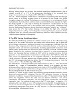
Fig. 8 shows the plots of AR parameter patterns from the six defective bearings. The first
column displays the six training patterns, which is the first one of the eight data sets from
each bearing type. The second column illustrates some of the other seven test patterns,
where the solid lines represent data from the first collection batch and the dotted lines are
from the second batch. As can be seen from Fig. 8, the profiles of the AR parameter patterns
within each group are very similar. Only a few deviations can be seen between the first and
second batches. The deviations come from the very sensitive but inevitable internal
structure changes of the setup during the bearing attachment and detachment operations
between the two data collections.
The experimental procedure began with using the first pattern of all the conditions for
training and then randomly testing the other seven patterns. In addition, the modified
ARTMAP network was designed to provide two suggested fault patterns (i.e., the outputs of
the first two activated nodes from the F
2
field). Table 2 summarizes the test results on
diagnosing the 42 test patterns. The first column of Table 2 for each bearing type is the first
identified fault from the network. It shows only 3 of the 42 test cases were mismatched in
the first guess but they were then picked up correctly by the network in the second guess
(see bold-face numbers in Table 2). Interestingly, these three mismatched patterns were from
Artificial Neural Networks - Industrial and Control Engineering Applications

432
the second batch. If the profiles of Bearings 4 and 5 in the second batch (the dotted profiles
in the second column of Fig. 8) were compared, then one could see the test patterns of
Bearing 4 from the second batch were much closer to the training pattern of Bearing 5 than
that of Bearing 4. This is why the network recognized the test patterns of Bearing 4 as
Bearing 5 in its first guess. These test results clearly display the capability and reliability of

the ARTMAP-based diagnostic system and the robustness of using AR parameter patterns
to represent vibration signals. For the efficiency of the ARTMAP training, the training time
of one 31-point AR parameter pattern was less than one second on a PC.

Bearing 1
0
0.5
1
1 4 7 1013161922252831
AR Order
Bearing 2
0
0.5
1
1 4 7 1013161922252831
AR Order
Bearing 3
0
0.5
1
1 4 7 1013161922252831
AR Order
Bearing 4
0
0.5
1
1 4 7 1013161922252831
AR Order
Bearing 5
0

0.5
1
1 4 7 1013161922252831
AR Order
Bearing 6
0
0.5
1
1 4 7 1013161922252831
AR Order
B1 Test Patterns
0
0.5
1
1 4 7 10 13 16 19 22 25 28 31
AR Order
B2 Test Patterns
0
0.5
1
1 4 7 10 13 16 19 22 25 28 31
AR Order
B3 Test Patterns
0
0.5
1
1 4 7 10 13 16 19 22 25 28 31
AR Order
B4 Test Patterns
0

0.5
1
1 4 7 10 13 16 19 22 25 28 31
AR Order
B5 Test Patterns
0
0.5
1
1 4 7 10 13 16 19 22 25 28 31
AR Order
B6 Test Patterns
0
0.5
1
1 4 7 10 13 16 19 22 25 28 31
AR Order

Fig. 8. AR parameters patterns of defective bearings
4. Summary and conclusions
This paper presents an integrated Intelligent Diagnostic System (IDS). Several unique
features have been added to ISDS, including the advanced vibration trending techniques,
the data reduction and features extraction through AR parametric model, the multi-channel
and on-line capabilities, the user-friendly graphical display and control interface, and a
unique machine diagnostic scheme through the modified ARTMAP neural network.
Intelligent Vibration Signal Diagnostic System Using Artificial Neural Network

433
Based on the ART2 architecture, a modified ARTMAP network is introduced. The modified
ARTMAP network is capable of supervised learning. In order to test the performance and
robustness of the modified ARTMAP network in ISDS, an extensive bearing fault

experiment has been conducted. The experimental results show ISDS is able to detect and
identify several machine faults correctly (e.g., ball bearing defects in our case).
5. Appendix
5.1 Time series autoregressive (AR) parametric model
According to the features representation requirements in signal pattern recognition, if the
features shown by raw data are ambiguous, then it is necessary to use a preprocessor or
transformation method on the raw data. Such a preprocessor should have feature extraction
capability that can invariably transfer raw data from one domain to another. The objective of
this preprocessing stage is to reveal the characteristics of a pattern such that the pattern can
be more easily identified.
The most important feature provided in vibration signals is frequency. Therefore, the
characteristics of vibration signals can be shown clearly in the frequency domain.
Traditionally, the Fast Fourier Transform (FFT) based spectral estimators are used to estimate
the power spectral density (PSD) of signals. Recently, many parameter estimation methods
have been developed. Among them, the autoregressive (AR) modeling method is the most
popular (Gersch & Liu, 1976). The major advantage of using the parametric spectral estimation
method is its ability to translate a time signal into both frequency (PSD) domain and parameter
domain. In addition, parametric spectrum estimation is based on a more realistic assumption
and does not need a long data record to get a high resolution spectrum.
5.2 Parametric autoregressive spectral estimation
Vibration signals can be treated as if they were generated from a time series random
process. Now consider a time series x
n
,

, , ,0, ,
n
xn
=
−∞ ∞……

(A.1)
where the observed interval is from n = 1, , N. The autoregressive model of x
n
is given in
Equation (A.2).

1122nn n
p
n
p
n
xax ax ax e
−− −
=
−− −− +… (A.2)
where e
n
is the prediction error, and p is the order of the model. The parametric spectrum
may be computed by plugging all p a
k
parameters into the theoretical power spectral density
(PSD) function defined from Equation (A.3).

()
2
2

=1
2
()

1+ exp - 2
11
22
1
AR
P
k
k
t
Pf
aifkt
f
t
S
σ
π
Δ
=
⎛⎛
Δ
⎜⎜
⎝⎝
−≤≤
Δ=
Σ
(A.3)