Heat Transfer Engineering Applications Part 6 ppt

Experimental and Numerical Evaluation of
Thermal Performance of Steered Fibre Composite Laminates

139
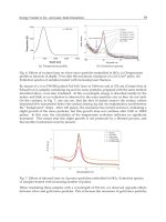
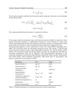
For variable-stiffness panels a family of curves corresponding to various values of T
1
(from
0º to 90º in increments of 15º) is plotted in Figure 12. The lowest normalized value of stress-
resultant is 0.185, and is obtained for a variable stiffness configuration of T
0
= 85º and T
1
= 0º,
with normalized longitudinal deflection value of about 1.127. This value is 68% lower than
the lowest value of 0.577 obtained with a straight-fiber configuration, but with 12% increase
of normalized longitudinal deformation. Most variable stiffness panels with T
0
= 0º and T
1
in
the range of 0º to 45º have a higher stress resultant than the corresponding straight-fiber
configurations.

0.95 1 1.05 1.1 1.15 1.2 1.25 1.3 1.35
0
0.5
1
1.5
2
2.5
Normalized longitudinal deformation

Normalized stress resultant x-dir

Fig. 12. Normalized longitudinal stress resultant for [0 ±<T
0
/T
1
>/90± <T
0
/T
1
>]
S
6. Thermal testing of variable stiffness laminates
The thermal-structural responses of two variable stiffness panels and a third cross-ply panel
are evaluated under thermal loads. A brief description of the variable stiffness panels and
their fiber orientation angles is given, along with an overview of the thermal test setup and
instrumentation. Results of these tests are presented and discussed, and include measured
thermal strains and calculated coefficients of thermal expansion.
6.1 Fiber tow path definition
The layups of the three composite panels tested in this study are described herein. The two
variable stiffness panel layups are [±45/(±

)
4
]
s
, where the steered fiber orientation angle


varies linearly from ±60º on the panel axial centerline, to ±30º near the panel vertical edges

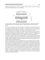
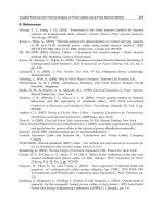
30.5 cm away. The curvilinear tow paths that the fiber placement machine followed during
fabrication of these variable stiffness panels are shown in Figure 13. One panel has all 24,
0.32-cm-wide tows placed during fabrication. This results in significant tow overlaps and
thickness buildups on one side of the panel, and therefore it is designated as the panel with
T
1
= 0
o
T
1
= 15
o
T
1
= 90
o

Heat Transfer – Engineering Applications

140
overlaps. The fiber placement system’s capability to drop and add individual tows during
fabrication is used to minimize the tow overlaps of the second variable stiffness panel,
which is designated as the panel without overlaps. The third panel has a straight-fiber
[±45]
5s
layup and provides a baseline for comparison with the two variable stiffness panels.
The overall panel dimensions are 66.0 cm in the axial direction, and 62.2 cm in the transverse
dimension, as indicated by the dashed lines in the figure. Further details of the panel
construction are given in (Wu, 2006).
6.2 Test setup and instrumentation

The thermal test was performed in an insulated oven with feedback temperature control.
Electrical resistance heaters and a forced-air heater unit were used to heat the enclosure.
Perforated metal baffles were used to evenly distribute hot air over the back surface of the
panel. The oven’s front was glass to allow observation of the panel using shadow moiré
interferometry. The panel was supported inside the oven with fixtures that restricted its
rigid-body motion but allowed free thermal expansion. The panel was placed on two small
quartz rods that prevented direct contact with the lower heated platen. The panel surfaces
were supported between quartz cones and spring-loaded steel probes with low axial
stiffnesses.


Fig. 13. Variable stiffness panel tow paths.
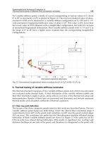
Each composite panel was gradually heated from room temperature up to approximately 65
ºC. A feedback control system provided closed-loop, real-time thermal control based on
readings from five K-type thermocouples on the heated platens and air inlet surrounding
the panel. These separate data were then averaged into a single temperature provided to the
control system. The thermocouples used in this study have a measurement uncertainty of ±1
ºC. For a thermal test, the control temperature inside the oven was first raised to 32 ºC and
Experimental and Numerical Evaluation of
Thermal Performance of Steered Fibre Composite Laminates

141
held there for 5 minutes. After the hold period, the control temperature was raised at 1
ºC/min. to a maximum of 65 ºC and held there for 20 minutes before the test was ended.
The solid line in Figure 14 shows the average of the five control thermocouples plotted
against time for a typical test.


Fig. 14. Temperature profiles for thermal tests.

Fig. 15. Composite panel instrumentation.

Heat Transfer – Engineering Applications

142
The panel response was measured during the thermal test with thermocouples and strain
gages, and these data were collected using a personal computer-based system. Panel front
and back surface temperatures were measured with five pairs of K-type thermocouples. The
average panel temperature is shown as a function of time as the dashed line in Figure 14.
The thermocouples, denoted as black-filled circles, are located at the corners and center of a
30.5-cm square centered on the panel, as shown in Figure 15.
Back-to-back pairs of electrical-resistance strain gages (each with a nominal ±1 percent
measurement error) are bonded to the panel surfaces using the procedures described in
(Moore, 1997). The locations of the strain gage pairs on each panel are also shown in Figure
15. The strain gages measure either axial strains (the open circles in the figure), or both axial
and transverse strains (the gray filled circles), and are deployed along the top edge, and
axial and transverse centerlines of the panels. The closely spaced axial gage pairs (locations
9, 10 and 11) on the panel with overlaps span a region of varying laminate thickness along
the transverse centerline. In addition to the axial gage pairs along the upper edge of the
baseline panel, biaxial gages are fitted at locations 4, 7 and 10 along the axial centerline.
6.3 Test results
The heating profile shown in Figure 14 is applied to the panels, and the resulting panel
thermal response is measured. An initial thermal cycle is performed for each panel to fully
cure the adhesives used to attach the strain gages to the panels. Since the strain gage
response is dependent on both its operating temperature and the motion of the surface to
which it is bonded, the thermal output of the strain gages themselves (Anon., 1993;
Kowalkowski et al., 1998) must first be determined. Strain data are recorded for gages
bonded to Corning ultralow-expansion titanium silicate (coefficient of thermal expansion 0 ±
3.06 x 10-8 cm/cm/ºC) blocks that are subjected to the same thermal loading. After

completion of each thermal test, this thermal output measurement is then subtracted from
the total (apparent) strain of each strain gage recorded during the test to obtain the actual
mechanical strains presented below.
6.3.1 Variable stiffness panels
Measured axial and transverse strains at the center (gage location 7) of the panel with
overlaps are plotted against the panel temperature in Figure 16 for a representative thermal
test. The plotted strains on the front and back panel surfaces are proportional to the
temperature, and are qualitatively similar to the responses at the other panel gage locations.
The membrane strain at the laminate mid-plane is defined as the average strain from a back-
to-back gage pair. The panel’s local coefficient of thermal expansion (CTE) at that gage
location is then defined as the linear best-fit slope of the membrane strain as a function of
temperature. Using the panel center strains shown in Figure 16, the measured axial CTE
there is 9.11 x 10-6 cm/cm/ºC, and the transverse CTE is 0.11 x 10-6 cm/cm/ºC (units of 1 x
10-6 cm/cm are denoted as με or microstrain). Note that these local CTEs for the variable
stiffness panels are dependent on the non-uniform fiber orientation angles, and may not be
equal to straight-fiber CTEs calculated using classical lamination theory.
The maximum measured strains at each of the 12 gage locations on the panel with overlaps are
plotted in Figure 17, with the corresponding axial CTEs shown in Figure 18. The axial CTEs
increase from –3.98 με/ºC near the edges (

=±30º) to 10.67 με/ºC along the axial centerline
(

=±60º). Transverse CTEs are also plotted in the figure and range from –0.94 to 1.35 με/ºC. In
Experimental and Numerical Evaluation of
Thermal Performance of Steered Fibre Composite Laminates

143
general, the fiber-dominated ±30º layups near the panel edges have low axial CTEs and high
transverse CTEs. The opposite is true for the matrix-dominated ±60º laminates on the panel

axial centerline, which have high axial CTEs and low transverse CTEs.


Fig. 16. Strain vs. temperature at center of panel with overlaps.


Fig. 17. Maximum strains for panel with overlaps.

Heat Transfer – Engineering Applications

144



Fig. 18. CTEs for panel with overlaps.



Fig. 19. Strain vs. temperature at center of panel without overlaps.
Experimental and Numerical Evaluation of
Thermal Performance of Steered Fibre Composite Laminates

145
The 20-ply laminate on the transverse centerline 12.7 cm on either side of the panel center
has a [±45/(±48)4]s layup. However, the measured axial CTEs (6.35 and 5.33 με/ºC) at gage
locations 6 and 8 there are much higher than the corresponding transverse CTEs (1.35 and
0.92 με/ºC). Since the CTEs of an [±45]5s orthotropic cross-ply laminate should all be equal,
the observed differences strongly suggest that the variable stiffness laminate CTEs can be
highly sensitive to relatively small changes in the fiber orientation angles.

Fig. 20. Maximum strains for panel without overlaps.
Measured axial and transverse strains on the front and back surfaces of the center of the
panel without overlaps are shown plotted against the corresponding panel temperature in
Figure 19. The axial and transverse strains at the maximum test temperature at each of the
10 strain gage locations on this panel are shown in Figure 20. The axial and transverse CTEs
plotted in Figure 21 are then calculated from the membrane strains. Axial CTEs for the panel
without overlaps range from –2.14 με/ºC near the panel edges to 9.16 με/ºC along the axial
centerline, with transverse CTEs ranging from –0.79 με/ºC on the axial centerline to 9.07
με/ºC on the transverse centerline near the panel edge. The CTEs for the panel without
overlaps are much more symmetric with respect to the panel axial and transverse centerlines

Heat Transfer – Engineering Applications

146
than those described previously for the panel with overlaps. However, similar qualitative
trends are observed in the plotted CTEs for both panels.

Fig. 21. CTEs for panel without overlaps.
6.3.2 Baseline panel
Front and back surface axial and transverse strains at the baseline panel center are plotted as
functions of the panel temperature in Figure 22. The measured strains are linear and very
nearly equal, which is to be expected since the [±45]5s layup has the same response in both
the axial and transverse directions. The range of measured CTEs for the baseline panel is
from 2.34 to 3.40 με/ºC, with an average CTE of 2.92 με/ºC. The corresponding standard
deviation is 0.32 με/ºC, resulting in an 11 percent coefficient of variation. The maximum
temperature for the baseline panel thermal test is about 3.9 ºC lower than the maximum
temperature for the variable stiffness panels because the heating profile was terminated
when the temperature reached 65 ºC.
Experimental and Numerical Evaluation of
Thermal Performance of Steered Fibre Composite Laminates

147








Fig. 22. Strain vs. temperature at center of baseline panel.
6.4 Summary
The measured strain response at each gage location on each of the composite panels is
generally linear with increasing temperature. The membrane strain at each gage location is
defined and used to compute the laminate CTE at that location. The measured axial CTEs

for both variable stiffness panels are lowest near the panel edges and increase to their
maximum values along the axial centerline, while the transverse CTEs show the opposite
behavior. This corresponds to the fiber-dominated ±30º layup towards the panel edges and a
matrix-dominated ±60º layup on the axial centerline. For a given orientation, the measured
CTEs along the panel axial centerlines are all fairly close to one another. This is as expected,
since the fiber orientation angle varies along the panel transverse axis, with only the ply
shifts contributing to any axial fiber orientation angle variation.
7. References
Abdalla, M, Gürdal, Z and Abdelal, G. (2009). Thermomechanical response of variable
stiffness composite panels. Journal of Thermal Stresses, Vol. 32, No. 1, pp. (187 –
208).

Heat Transfer – Engineering Applications

148
Anon. (1993). Strain Gage Thermal Output and Gage Factor Variation with Temperature.
TN-504-1, Measurements Group, Inc., Raleigh, North Carolina.
Banichuk, NV. (1981). Optimization Problems for Elastic Anisotropic Bodies. Archive of
Mechanics, 33, 1981, pp. (347-363).
Banichuk, NV and Sarin, V. (1995). Optimal Orientation of Orthotropic Materials for Plates
Designed Against Buckling. Structural and Multidisciplinary Optimization, Vol. 10,
No. 3-4, 1995, pp. (191-196).
Bogetti, T. (1989). Process-Induced Stress and Deformation in Thick-Section Thermosetting
Composites. Technical Report CCM-89-32, Center for Composite Materials,
University of Delaware, Newark, Delaware, 1989.
Bogetti, T and Gillespie, J. (1992). Process-Induced Stress and Deformation in Thick-Section
Thermoset composite Laminates”, Journal of Composite Materials, Vol. 26, No. 5, pp.
(626-660).
Cole, K, Hechler, J and Noël, D. (1991). A New Approach to Modelling the Cure Kinetics of
Epoxy Amine Thermosetting Resin. 2. Application to a Typical System Based on

Bis[4-diglycidylamino)phenyl]methane and Bis(4-aminophenyl) Sulphone”,
Macromolecules. Vol. 24, No. 11, pp. (3098-3110).
Dusi, M, Lee, W, Ciriscioli, P and Springer, G. (1987). Cure Kinetics and Viscosity of Fiberite
976 Resin,” Journal of Composite Materials. Vol. 21, No. 3, pp. (243-261).
Duvaut, G, Terrel, G, Léné, F and Verijenko, V. (2000). Optimization of Fiber Reinforced
Composites. Composite Structures, Vol. 48, 2000, pp. (83-89).
Gürdal, Z and Olmedo, R. (1993). In-Plane Response of Laminates with Spatially Varying
Fiber Orientations: Variable Stiffness Concept. AIAA Journal, Vol. 31, (4), pp. (751-
758), 0001-1452.
Gürdal, Z, Haftka, RT and Hajela, P. (1999). Design and Optimization of Laminated Composite
Materials. John Wiley & Sons, Inc., New York, NY.
Gürdal, Z, Tatting, BF and Wu, KC. (2008). Variable stiffness composite panels: Effects of
stiffness variation on the in-plane and buckling response. Composite: Part A, Vol. 39,
2008, pp. (911-922).
Hetnarski, RB. (1996). Thermal stresses (I–IV). Amsterdam: Elsevier Science Pub. Co.
Hughes, T, Levit, I and Winget, J. (1982). Unconditionally stable element-by-element implicit
algorithm for heat conduction analysis. U.S. Applied Mechanics Conference,
Cornell University, Ithaca, USA.
Johnston, A. (1997). An Integrated Model of the Development of Process-Induced Deformation in
Autoclave Processing of Composite Structures. PhD dissertation, University of British
Columbia.
Levitsky, M and Shaffer, B. (1975). Residual Thermal Stresses in a Solid Sphere Cast From a
Thermosetting Material. Journal of Applied Mechanics, pp. (651-655).
Kowalkowski, M, Rivers, HK and Smith, RW. (1998). Thermal Output of WK-Type Strain
Gauges on Various Materials at Elevated and Cryogenic Temperatures. NASA TM-
1998-208739, October 1998.
Lee, W, Loos, A and Springer, S. (1982). Heat of Reaction, Degree of Cure, and Viscosity of
Hercules 3501-6 Resin”, Journal of Composite Materials. Vol. 16, pp. (510-520).
Experimental and Numerical Evaluation of
Thermal Performance of Steered Fibre Composite Laminates

149
Mittler, G, Klima, R, Alapin, B, et al. (2003). Determination and application of thermo-
mechanical characteristics for the optimization of refractory linings. STAHL UND
EISEN Vol. 123, No. 11 pp. (109–12).
Moore, T. (1997). Recommended Strain Gage Application Procedures for Various Langley
Research Center Balances and Test Articles. NASA TM-110327, March 1997.
Obata, Y and Noda, N. (1993). Unsteady thermal stresses in a functionally gradient material
plate - Analysis of one-dimensional unsteady heat transfer problem. Japan Society
of Mechanical Engineers, Transactions A (ISSN 0387-5008), Vol. 59, No. 560, pp.
(1090-1096).
Olmedo, R and Gürdal, Z. (1993). Buckling Response of Laminates with Spatially Varying
Fiber Orientations, Proceedings of the 34
th
AIAA/ASME/ASCE/AHS/ASC
Structures, Structural Dynamics and Materials (SDM) Conference, La Jolla, CA,
April 1993.
Pedersen, P. (1991). On Thickness and Orientation Design with Orthotropic Materials.
Structural Optimization, Vol. 3, 1991, pp. (69-78).
Pedersen, P. (1993). Optimal Orientation of Anisotropic Materials, Optimal Distribution of
Anisotropic Materials, Optimal Shape Design with Anisotropic Materials, Optimal
Design for a Class of Non-linear Elasticity. Optimization of Large Structural Systems,
Ed. Rozvany, G. I. N., Vol. 2, 1993, pp. (649-681).
Scott, P. (1991). Determination of Kinetic Parameters Associated with the Curing of
Thermoset Resins Using Dielectric and DSC Data”, Composites: Design, Manufacture,
and Application, ICCM/VIII, Honolulu, 1991.
Segerlind, LJ. (1984). Applied Finite Element Analysis. John Wiley & Sons.
Setoodeh, S, Abdalla, M and Gürdal, Z. (2006). Design of variable–stiffness laminates using
lamination parameters. Composites Part B: Engineering. Vol. 37, No. 4-5, pp. (301-
309).

Setoodeh, S, Abdalla, M and Gürdal, Z. (2007). Design of variable stiffness composite panels
for maximum fundamental frequency using lamination parameters. Composite
Structures. Vol. 81, No. 2, pp. (283-291).
Setoodeh, S, Abdalla, M, IJsselmuiden, S and Gürdal, Z. (2009). Design of variable-stiffness
composite panels for maximum buckling load. Composite Structures. Vol. 87, No. ,
pp. (109-117).
Thornton, EA. (1992). Thermal structures and materials for high-speed flight. American Institute
of Aeronautics and Astronautics.
Trujillo, D. (1977). An unconditionally stable explicit algorithm for structural dynamics.
International Journal of Numerical Methods Engineering, Vol. 1, pp. (1579-1592).
Twardowski, T, Lin, S and Geil, P. (1993). Curing in Thick Composite Laminates:
Experiments and Simulation”, Journal of Composite Materials. Vol. 27, No. 3, pp.
(216-250).
White, S and Hahn, H. (1992). Process Modelling of Composite Materials: Residual Stress
Development during Cure. Part I. Model Formulation”, J. of Composite Materials.
Vol. 26, No. 16,pp. ( 2402-2422).

Heat Transfer – Engineering Applications

150
Wu, KC. (2006). Thermal and Structural Performance of Tow-Placed, Variable Stiffness
Panels. ISBN 1-58603-681-5, Delft University Press/IOS Press, Amsterdam, The
Netherlands, 2006.
Zienkiewicz, O, Hinton, E, Leung, K and Taylor, R. (1980). Staggered time marching
schemes in dynamic soil analysis and a selective explicit extrapolation algorithm.
Second International Symposium on Innovative Numerical Analysis in Applied
Engineering Sciences, Canada.
7
A Prediction Model for
Rubber Curing Process

Shigeru Nozu
1
, Hiroaki Tsuji
1
and Kenji Onishi
2

1
Okayama Prefectural University
2
Chugoku Rubber Industry Co. Ltd.
Japan
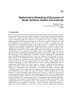
1. Introduction
A prediction method for rubber curing process has historically received considerable
attention in manufacturing process for rubber article with relatively large size. In recent
years, there exists increasing demand for simulation driven design which will cut down the
cost and time required for product development. In case of the rubber with relatively large
dimensions, low thermal conductivity of the rubber leads to non-uniform distributions of
the temperature history, which results in non-uniform cure state in the rubber. Since rubber
curing process is an exothermic reaction, both heat conduction equation and expressions for
the curing kinetics must be solved simultaneously.
1.1 Summary of previous works
In general, three steps exist for rubber curing process, namely, induction, crosslinking and
post-crosslinking (e.g. Ghoreishy 2009). In many previous works, interests are attracted in
the former two, and a sampling of the relevant literature shows two types of the prediction
methods for the curing kinetics.
First type of the method consists of a set of rate equations describing chemical kinetics.
Rubber curing includes many complicated chemical reactions that might delay the
modelling for practical use. Coran (1964) proposed a simplified model which includes the
acceleration, crosslinking and scorch-delay. After the model was proposed, some

improvements have been performed (e.g. Ding et al, 1996). Onishi and Fukutani
(2003a,2003b) performed experiments on the sulfur curing process of styrene butadiene
rubber with nine sets of sulfur/CBS concentrations and peroxide curing process for several
kinds of rubbers. Based on their results, they proposed rate equation sets by analyzing the
data obtained using the oscillating rheometer operated in the range 403 K to 483 K at an
interval of 10 K. Likozar and Krajnc (2007) proposed a kinetic model for various blends of
natural and polybutadiene rubbers with sulphur curing. Their model includes post-
crosslinking chemistry as well as induction and crosslinking chemistries. Abhilash et al.
(2010) simulated curing process for a 20 mm thick rubber slab, assuming one-dimensional
heat conduction model. Likazor and Krajnc (2008, 2011) studied temperature dependencies
of relevant thermophysical properties and simulated curing process for a 50 mm thick
rubber sheet heated below, and good agreements of temperature and degree of cure have
been obtained between the predicted and measured values.

Heat Transfer – Engineering Applications

152
The second type prediction method combines the induction and crosslinking steps in series.
The latter step is usually expressed by an equation of a form dε/dτ = f(ε,T), where ε is the
degree of cure, τ is the elapsed time and T is the temperature. Ghoreishy (2009) and Rafei et
al. (2009) reviewed recent studies on kinetic models and showed a computer simulation
technique, in which the equation of the form dε/dτ= f(ε,T) is adopted. The form was
developed by Kamal and Sourour (1973) then improved by many researchers (e.g. Isayev
and Deng, 1987) and recently the power law type models are used for non-isothermal, three-
dimensional design problems (e.g. Ghoreishy and Naderi, 2005).
Temperature field is governed by transient, heat conduction equation with internal heat
generation due to the curing reaction. Parameters affecting the temperature history are
dimensions, shape and thermophysical properties of rubbers. Also initial and boundary
conditions are important factors. Temperature dependencies of relevant thermophysical
properties are, for example, discussed in Likozar and Krajnc (2008) and Goyanes et

al.(2008). Few studies have been done accounting for the relation between curing
characteristics and swelling behaviour (e.g. Ismail and Suzaimah, 2000). Most up-to-date
literature may be Marzocca et al. (2010), which describes the relation between the
diffusion characteristics of toluene in polybutadiene rubber and the crosslinking
characteristics. Effects of sulphur solubility on rubber curing process are not fully clarified
(e.g. Guo et al., 2008).
Since the mechanical properties of rubbers strongly depend on the degree of cure, new
attempts can be found for making a controlled gradient of the degree of cure in a thick
rubber part (e.g. Labban et al., 2007). To challenge the demand, more precise considerations
for the curing kinetics and process controls are required.
1.2 Objective of the present chapter
As reviewed in the above subsection, many magnificent experimental and theoretical
studies have been conducted from various points of view. However, few fundamental
studies with relatively large rubber size have been done to develop a computer simulation
technique. Nozu et al. (2008), Tsuji et al. (2008) and Baba et al. (2008) have conducted
experimental and theoretical studies on the curing process of rubbers with relatibely large
size. Rubbers tested were styrene butadiene rubbers with different sulphur concentration,
and a blend of styrene butadiene rubber and natural rubber. Present chapter is directed
toward developing a prediction method for curing process of rubbers with relatively large
size. Features of the chapter can be summarized as follows.
1. Experiments with one-dimensional heat conduction in the rubber were planned to
consider the rubber curing process again from the beginning. Thick rubber samples
were tested in order to clarify the relation between the slow heat penetration in the
rubber and the onset and progress of the curing reaction.
2. The rate equation sets derived by Onishi and Fukutani (2003a,2003b) were adopted for
describing the curing kinetics.
3. Progress of the curing reaction in the cooling process was studied.
4. Distributions of the crosslink density in the rubber were determined from the
equation developed by Flory and Rehner (1943a, 1943b) using the experimental
swelling data.

5. Comparisons of the distributions of the temperature history and the degree of cure
between the model calculated values and the measurements were performed.

A Prediction Method for Rubber Curing Process

153
2. Experimental methods
The most typical curing agent is sulfur, and another type of the agent is peroxide (e.g.
Hamed, 2001). In this section, summary of our experimental studies are described. Two
types of curing systems were examined. One is the styrene butadiene rubber with
sulfur/CBS system (Nozu et al., 2008). The other is the blend of styrene butadiene rubber
and natural rubber with peroxide system (Baba et al., 2008).
2.1 Styrene Butadiene Rubber (SBR)
Figure 1 illustrates the mold and the positions of the thermocouples for measuring the
rubber temperatures (rubber thermocouples). A steel pipe with inner diameter of 74.6 mm
was used as the mold in which rubber sample was packed. On the outer surface of the mold,
a spiral semi-circular groove with diameter 3.2 mm was machined with 9 mm pitch, and
four sheathed-heaters with 3.2 mm diameter, a ~ d, were embedded in the groove. On the
outer surface of the mold, silicon coating layer was formed and a grasswool insulating
material was rolled. The method described here provides one-dimensional radial heat
conduction excepting for the upper and lower ends of the rubber.
Four 1-mm-dia type-E sheathed thermocouples, A ~ D, were located in the mold as the wall
thermocouples. Four 1-mm-dia Type-K sheathed thermocouples were equipped with the
mold to control the heating wall temperatures. The top and bottom surfaces were the
composite walls consisting of a Teflon sheet, a wood plate and a steel plate to which an
auxiliary heater is embedded.
To measure the radial temperature profile in the rubber, eight type-J thermocouples were
located from the central axis to the heating wall at an interval of 5 mm. At the central axis
just below 60 mm from the mid-plane of the rubber, a type-J thermocouple was also located
to measure the temperature variation along the axis. All the thermocouples were led out

through the mold and connected to a data logger, and all the temperature outputs were
subsequently recorded to 0.1 K.
Styrene butadiene rubber (SBR) was used as the polymer. Key ingredients include sulfur as
the curing agent, carbon blacks as the reinforced agent. Ingredients of the compounded
rubber are listed in Table 1, where sulfur concentrations of 1 wt% and 5wt% were prepared.
To locate the rubber thermocouples at the prescribed positions, rubber sheets with 1 and 2
mm thick were rolled up with rubber thermocouples and packed in the mold.
Two curing methods, Method A and Method B, were adopted. Method A is that the heating
wall temperature was maintained at 414K during the curing process. Method B is that the
first 45 minutes, the wall temperature was maintained at 414K, then the electrical inputs to
the heaters were switched off and the rubber was left in the mold from 0 to 75 minutes at an
interval of 15 minutes to observe the progress of curing without wall heating. By adopting
the Method B, six kinds of experimental data with different cooling time were obtained. The
heater inputs were ac 200 volt at the beginning of the experiment to attain the quick rise of
to the prescribed heating wall temperature.
After each experiment was terminated, the rubber sample was brought out quickly from the
mold then immersed in ice water, and a thin rubber sheet with 5 mm thick was sliced just
below the rubber thermocouples to perform the swelling test. As shown in Fig.2, eight test
pieces at an interval of 5 mm were cut out from the sliced sheet. Each test piece has
dimensions of 3mm×3mm×5mm and swelling test with toluene was conducted.

Heat Transfer – Engineering Applications

154
Rubber
Sheathed
heater
Counte
r
heater

Thermocouple Steel plate
Mold
74.6
a
b
c
d
Wood Plate
Thermocouple
A
B
C
D
Thermal
insulator
Teflon sheet
Φ
74.6
240
120
Rubber thermocouples
60

Fig. 1. Experimental mold and positions of rubber thermocouples for SBR

Ingredients wt% wt%
Polymer (SBR) 53.8 51.6
Cure agent (Sulfur) 1.0 5.0
Vulcanization accelerator 0.9 0.9
Reinforcing agent (Carbon black) 31.9 30.6

Softner 8.0 7.6
Activator (1) 2.6 2.5
Activator (2) 0.5 0.5
Antioxidant (1) 0.5 0.5
Antioxidant (2) 0.3 0.3
Antideteriorant 0.3 0.5
Table 1. Ingredients of compounded SBR



Fig. 2. Cross sectional view at mid-plane of rubber sample

A Prediction Method for Rubber Curing Process

155
The crosslink density was evaluated from the equation proposed by Flory and Rehner
(1943a,1943b) using the measured results of the swelling test. In the present study, the
degree of cure

is defined by



[RX]/[RX]
0
(1)
where [RX] is the crosslink density at an arbitrary condition and [RX]
0
is that for the fully
cured condition obtained from our preliminary experiment.

2.2 Styrene Butadiene Rubber and Natural Rubber blend (SBR/NR)
Figure 3 illustrates cross-section of the mold which consists of a rectangular mold with inner
dimensions of 100mm×100mm×30 mm and upper and lower aluminum-alloy hot plates
heated by steam. Rubber sample was packed in the cavity.

x
0
30
5
L

Fig. 3. Experimental mold and hot plates for SBR/NR
Energy transfer in the rubber is predominantly one-dimensional, transient heat conduction
from the top and bottom plates to the rubber. To measure the through-the-thickness
temperature profile along the central axis in the rubber, type-J thermocouples were located
at an interval of 5 mm. Two wall thermocouples were packed between the hotplates and the
rubber. All the thermocouples were led out through the mold and connected to the data
logger, and the temperature outputs were subsequently recorded to 0.1K. The blend
prepared includes 70 wt% styrene butadiene rubber (SBR) and 30 wt% natural rubber (NR).
The peroxide was used as the curing agent. Ingredients are listed in Table 2.
To locate the rubber thermocouples at the prescribed positions rubber sheets with 5 mm
thick were superposed appropriately.
Experiments were conducted under the condition of the heating wall temperature 433 K by
changing the heating time in several steps from 50 to 120 minutes in order to study the
dependencies of the degree of cure on the heating time. After the heating was terminated,
the rubber was led out from the mold then immersed in ice water. The rubber was sliced 3
mm thick × 30 mm long in the vicinity of the central axis. Test pieces were prepared with
dimensions of 3mm×3mm×3mm at x= -10, -5, 0, 5 and 10 mm, where the coordinate x is

Heat Transfer – Engineering Applications

156
defined in Fig.3. The crosslink density was evaluated from the Flory-Rehner equation using
the measured swelling data.

Ingredients wt%
Polymer (SBR/NR) 70wt%SBR, 30wt%NR 86.2
Cure agent (Peroxide) 0.4
Reinforcing agent (Silica) 8.6
Processing aid 0.3
Activator 1.7
Antioxidant (1) 0.9
Antioxidant (2) 0.9
Coloring agent (1) 0.2
Coloring agent (2) 0.8
Table 2. Ingredients of compounded SBR/NR
3. Numerical prediction
Rubber curing processes such as press curing in a mold and injection curing are usually
operated under unsteady state conditions. In case of the rubber with relatively large
dimensions, low thermal conductivity of the rubber leads to non-uniform thermal history,
which results to non-uniform degree of cure.
The present section describes theoretical models for predicting the degree of cure for the
SBR and SBR/NR systems shown in the previous section. The model consists of solving one-
dimensional, transient heat conduction equation with internal heat generation due to
cureing reaction.
3.1 Heat conduction
Heat conduction equation with constant physical properties in cylindrical coordinates is

TTdQ
cr

rr r d











(2)
subject to
T = T
init
for τ = 0 (3a)
T = T
w
(τ) for τ > 0 and r = r
M
(3b)
T/r = 0 for τ > 0 and r = 0 (3c)
where
r
is the radial coordinate,

is the time，ρ is the density, c is the specific heat, λ is
the thermal conductivity, T
M

(τ) is the heating wall temperature, T
init
is the initial
temperature in the rubber and r
M
is the inner radius of the mold.
Heat conduction equation in rectangular coordinates is

2
2
TdTdQ
c
d
dx






(4)

A Prediction Method for Rubber Curing Process

157
subject to
T = T
init
for τ = 0 (5a)
T = T

w
(t) for τ > 0 and x = ±L (5b)
where x is the coordinate defined as shown in Fig. 3. The second term of the right hand sides
of equations (2) and (4), dQ/dτ, show the effect of internal heat generation expressed as
dQ/dτ = ρΔH dε/dτ (6)
where ΔΗ is the heat of curing reaction and

is the degree of cure.
3.2 Curing reaction kinetics
Prediction methods for the degree of cure ε in equations (2) and (4) have been derived by
Onishi and Fukutani(2003a,2003b) and the models are adopted in this chapter.
3.2.1 Styrene Butadiene Rubber (SBR)
Curing process of SBR with sulfur has been analyzed and modeled by Onishi and Fukutani
(2003a). A set of reactions is treated as the chain one which includes CBS thermal
decomposition.
Simplified reaction model is shown in Fig. 4, where α is the effective accelerator, N is the
mercapt of accelerator, M is the polysulfide, RN is the polysulfide of rubber, R* is the active
point of rubber, and RX is the crosslink site.


Fig. 4. Simplified curing model for SBR
The model can be expressed by a set of the following five chemical reactions.
k
1
a → N
k
2
N + a → M
k
3

M → RN + N
k
4
RN → R* + N
k
5
R* → RX
α
+α
(7)

Heat Transfer – Engineering Applications

158
which leads the following rate equation set
d[α]/dτ = - k
1
[α] – k
2
[N][α]
d[N]/dτ = k
1
[α] – k
2
[N][α] + k
3
[M] + k
4
[RN]
d[M]/dτ= k

2
[N][α] – k
3
[M]
d[RN]/dτ = k
3
[M] – k
4
[RN]
d[R*]/dτ = k
4
[RN] – k
5
[R*]
d[RX]/dτ = k
5
[R*]
where [α],[N],[M],[RN],[R*] and [RX] are the molar densities of appropriate species. Initial
conditions of equation (8) are [α] = 1 and zero conditions for the rest of species. Rate
constants k
i
(i = 1～5) in the set were expressed using the Arrhenius form as
k
i
= A
i
exp(-E
i
/RT) (9)
where A

i
is the frequency factor of reaction i, E
i
is the activation energy of reaction i, R is
the universal gas constant, T is the absolute temperature. Values of A
i
and E
i
are shown in
Table 3, where these values were derived from the analysis of the isothermal curing data
using the oscillating rheometer in the range 403 K to 483K at an interval of 10K (Onishi and
Fukutani, 2003a).


Sulfur
concentration
1 wt % 5 wt %
A
i
(1/s) E
i
/R (K) A
i
(1/s) E
i
/R (K)
1
k
1.034×10
7

1.166×10
4
1.387×10
-1
3.827
2
k
3.159×10
13
1.466×10
4
5.492×10
8
9.973
3
k
2.182×10
7
8.401×10
3
1.880×10
9
9.965
4
k
1.089×10
7
8.438×10
3
1.160×10

9
9.863
5
k
1.523×10
9
1.119×10
4
1.281×10
9
1.135×10

Table 3. Frequency factor and activation energy for SBR
3.2.2 Styrene butadiene rubber and natural rubber blend (SBR/NR)
Peroxide curing process for rubbers has been analyzed and modeled by Onishi and
Fukutani (2003b). Simplified reaction model is shown in Fig. 5, where R is possible crosslink
site of polymer, R* is active cure site, PR the polymer radical, RX* is the polymer radical
with crosslinks and RX is the crosslink site.
(8)

A Prediction Method for Rubber Curing Process

159
A
i
(1/s) E
i
/R (K)
1
k

1.243×10
8
1.095×10
4

2
k
1.007×10
15
1.826×10
4

3
k
9.004×10
2
6.768×10
3

4
k
2.004×10
6
8.860×10
3

5
k
1.000×10

-6
-3.171×10
3

Table 4. Frequency factor and activation energy for SBR/NR
k
1
k
2
k
5
k
3
k
4
(Peroxide)
(Peroxide)

Fig. 5. Simplified curing model for SBR/NR
The model can be expressed by a set of the following five chemical reactions.
k
1
R → R*
k
2
R* → PR

k
3
PR + R → RX*

k
4
RX* + R → RX + PR
k
5
PR + R*→ RX
which leads the following rate equation set
d[R]/dτ = - k
1
[R] – k
3
[PR][R] – k
4
[RX*][R]
d[R*]/dτ = k
1
[R] – k
2
[R*]
d[PR]/dτ = k
2
[R*] – k
3
[PR][R] + k
4
[RX*][R] – 2k
5
[PR]
2

d[RX*]/dτ = k
3
[PR][R] – k
4
[RX*][R]
d[RX]/dτ = k
4
[RX*][R] + k
5
[PR]
2

(10)
(11)

Heat Transfer – Engineering Applications

160
where [R], [R*], [PR], [RX*] and [RX] are the molar densities of appropriate species. Initial
conditions of equation (11) are [R] = 2 and zero conditions for the rest of species.
Rate constants k
i
(i = 1～5) are listed in Table 4, where the values were obtained from the
similar method conducted by Onishi and Fukutani (2003b).
3.3 Usage of the equations
For the SBR with sulfur curing system described in the previous section, we need to solve
heat conduction equation (2) together with rate equation set (8) to obtain cure state
distributions. Initial and boundary conditions for the temperatures were given by equation
(3). Initial concentration conditions are described below equation set (8). Similar method can

be adopted for estimating the SBR/NR system.


SBR
SBR/NR
Sulfur 1 wt% Sulfur 5wt%
Density ρ (kg/m
3
) 1.165×10
3
1.024×10
3

Thermal conductivity l (W/mK) 0.33 0.20
Specific heat capacity c (J/kgK) 1.84×10
3
1.95×10
3

Heat of reaction ΔΗ (J/kg) 1.23×10
4
3.99×10
4
2.78×10
4


Table 5. Physical properties used for prediction
The density ρ was determind using the mixing-rule. The thermal conductivity λ was
measured using the cured rubber at 293K. DSC measurements of the specific heat capacity c

and that of the heat of curing reaction ΔH for the rubber compounds were performed in the
range 293 K to 453 K. The theromophysical properties used for the prediction are tabulated
in Table 5. For the case of SBR with 5 wt% sulfur, a small correction of the specific heat
capacity was made in the range 385.9 K to 392.9K to account for the effect of the fusion heat
of crystallized sulfer. The solubility of sulfur in the SBR was assumed to be 0.8 wt% fom the
literature (Synthetic Rubber Divison of JSR, 1989). Heat conduction equations (2) and (4)
were respectively reduced to systems of simultaneous algebraic equations by a control-
volume-based, finite difference procedure. Number of control volumes were 37 for SBR with
37.3 mm radius and 30 for SBR/NR with 30 mm thick. Time step of 0.5 sec was chosen after
some trails.
4. Comparison with experimental data
4.1 Styrene Butadiene Rubber (SBR)
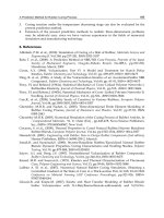
Figure 6 shows the temperature profile for the cured rubber with Method A, where solid
and dashed lines respectively show the numerical results and the measured heating wall
temperature. Symbols present measured rubber temperatures. In the figure for the
measured temperatures, typical one-dimensional transient temperature field can be
observed and it takes about 180 minutes to reach T
R
to the final temperature T
w
.
Comparisons of the measured and predicted temperatures show good agreements between
them. Also, the measured temperature difference along the axis between the positions at
mid-cross section and that at 60 mm downward was less than 0.5 K. Since the difference is
considerably smaller as compared to the radial one, one-dimensional transient heat
conduction field is well established in the present experimental mold.

A Prediction Method for Rubber Curing Process

161

060120180
0
50
100
150
Elapsed time (min)
Temprerature T (℃)
Heating wall
0
10
20
30
35
r mm
Predicted T
R
Measured T
w


Fig. 6. Temperature profile for cured SBR, Method A


060120180
0
50
100
150

Elapsed time

(min)
Temperature T (℃)
0
10
20
30
35
Heating wall
r mm
Predicted T
R
Measured T
w
Shoulder


Fig. 7. Temperature profile for SBR with 1 wt% sulfur, Method A
Figure 7 is the result of the compounded rubber with Method A. The temperature rise is
faster for the compounded rubber than for the cured one, and a uniform temperature field
is observed at about τ = 95 minutes. The former may be caused by the internal heat
generation due to curing reaction. The numerical results well follow the measured
temperature history.
Figure 8 shows the numerical results of the internal heat generation rate dQ/dτ and the
degree of cure ε corresponding to the condition of Fig.7. The dQ/dτ at each radial position r

Heat Transfer – Engineering Applications

162

shows a sharp increase and takes a maximum then decreases moderately. It can also be seen
that the onset of the heat generation takes place, for example, at τ = 15 minutes for r = 35
mm, and at τ = 65 minutes for r = 0mm. This means that the induction time is shorter for
nearer the heating wall due to slow heat penetration. Another point to note here is that the
symmetry condition at r = 0, equation (3c), leads to the rapid increase of T
R
near r = 0 after τ
= 60 minutes is reached as shown in Fig.7. The degree of cure ε increases rapidly just after
the onset of curing, then approaches gradually to 1 as shown in the lower part of Fig.8.
Figure 9 shows the profiles of rubber temperature and that of degree of cure, both are model
calculated results. An overall comparison of the Figs. 9(a) and 9(b) indicates that the
progress of the curing is much slower than the heat penetration. The phenomenon is
pronounced in the central region of the rubber. Temperature profiles at τ = 90 and 105
minutes were almost unchanged, thus the two profiles can not be distinguished in the
figure.



0
1
2
3
4
060120180
0.0
0.5
1.0
Heat generation rate dQ/d

(W/m

3
)
r = 0 mm
2030
35
10
Degree of cure 
35
30
20
10
r = 0 mm
Elapsed time

(min)
×10
4



Fig. 8. Heat generation rate dQ/dτ and degree of cure ε for SBR with 1 wt% sulphur,
Method A, corresponding to Fig.7

A Prediction Method for Rubber Curing Process

163


010203040
0.0

0.5
1.0
010203040
0
50
100
150
Degree of cure

75
60
45
90
Radial distance r (mm)
= 105 min
r = r
M
30 15
Temperature T (℃)
15
r = r
M
30
45
60
Radial distance r (mm)
75
= 0 min
= 90, 105 min

(a) Rubber temperature (b) Degree of cure

Fig. 9. Profiles of rubber temperature and degree of cure, SBR with 1wt% sulphur, Method
A, corresponding to Figs.7 and 8



060120
0
50
100
150
Temperature T 　(℃)
Heater Off
Elapsed time  (min)
r (mm)
0
10
20
30
35
Heating wall


Fig. 10. Profile of rubber temperature for SBR with 1wt% sulfur, Method B