Desalination Trends and Technologies Part 11 docx

Reject Brine Management

239
amount of dissolved oxygen available for the marine organisms. Other harmful chemicals that
may be present in the reject brine such as hydrogen sulfide and chloride may have negative
effect if the brine is not treated before disposal. In addition, the continuous disposal of reject
brine into water body near the desalination plants could, in the long run, affect the suitably of
the feed water. This is especially true for small and rather closed water bodies such as the
Arabian Gulf, where most of the desalination activities in the world take place.
2.2 Deep well injection
Deep well injection is often considered for the disposal of industrial, municipal and liquid
hazardous wastes (Saripalli et al, 2000). In recent years, this approach has been given serious
consideration as an option for brine disposal from inland desalination plants, where surface
water discharge is not viable or very costly. Deep wells can offer a feasible and reliable
solution to disposing reject brine. However, deep wells are not feasible in areas subject to
earthquakes or where faults are present that can provide a direct hydraulic connection
between the receiving aquifer and an overlying potable aquifer (Mickely et al, 2006).
Therefore, prior to drilling any injection well, a careful assessment of geological conditions
must be conducted in order to determine the depth and location of suitable porous aquifer
reservoirs (Glator and Cohen, 2003). The capital cost for deep well injection is usually higher
than surface water disposal, where the latter method does not require long brine transport
pipelines. Although deep well injection may be a feasible option for reject brine disposal, it
still suffers from many drawbacks such as the need for selecting a suitable well site; the
extra costs involved in conditioning the reject brine; corrosion and subsequent leakage in the
well casing; and seismic activity which could cause damage to the well and subsequently
contamination of groundwater (Glator and Cohen, 2003). Performance, design consideration
and modeling of deep well injection have been addressed by many researchers (Rhee and
Reible, 1993; Saripalli et al, 2000; Skehan and Kwiatkowski, 2000).
2.3 Evaporation ponds
This option has always been considered the most effective and economical method for brine
disposal for inland desalination plants, especially for dry, arid regions similar to those in

North Africa and Middle East. Inland plants in these regions are usually located in areas
known to have high dry weather, relatively high temperature and, consequently, high
evaporation rates. Ahmed et al. (2000) reviewed the relevant literature and presented the
design aspects of evaporation ponds, highlighting the importance of selecting the main
design parameters, namely surface area and pond depth. In another study (Ahmed et al,
2001), the authors surveyed the application of evaporation ponds in Arabian Gulf countries,
namely United Arab Emirates and Oman. The authors reported that the newer plants have
lined evaporation ponds, whereas the older ones have unlined disposal pits. The primary
environmental concern associated with evaporation pond disposal is pond leakage, which
may result in subsequent contamination of groundwater in the region. Recent evaporation
ponds are always lined with polyethylene or other polymeric materials to prevent leakage
and seepage of contaminants into the nearby groundwater.
A key factor in the effectiveness of evaporation ponds is the evaporation rate, which depends
heavily on the weather conditions, mainly humidity and surrounding temperature. Attempts
have been made, with limited success, to improve evaporation through the use of wind-aided
intensified evaporation (Gilron et al, 2003). This technique claims to increase the evaporation
rate by 50% for dry climate, but still depends on weather conditions. Improving the
Desalination, Trends and Technologies

240
evaporation rate could in principal reduce the size of the evaporation ponds and enhance their
efficiency and potential of application in many parts of the world. Although high temperature
and, consequently, high evaporation rates may speedup water reduction, evaporation ponds
still suffer from many drawbacks including the need for huge areas and the possibility of
contaminants dissipation into soil and groundwater.
3. Characteristics of reject brine
By definition, brine is any water stream in a desalination process that has higher salinity
than the feed. Reject brine is the highly concentrated water in the last stage of the
desalination process that is usually discharged as wastewater. Several types of chemicals are
used in the desalination process for pre- and post-treatment operations. These include:

Sodium hypochlorite (NaOCl) which is used for chlorination to prevent bacterial growth in
the desalination facility; Ferric chloride (FeCl
3
) or aluminum chloride (AlCl
3
), which are
used as flocculants for the removal of suspended matter from the water; anti-scale additives
such as Sodium hexameta phosphate (NaPO
3
)
6
are used to prevent scale formation on the
pipes and on the membranes; and acids such as sulfuric acid (H
2
SO
4
) or hydrochloric acid
(HCl) are also used to adjust the pH of the seawater. Due to the presence of these different
chemicals at variable concentrations, reject brine discharged to the sea has the ability to
change the salinity, alkalinity and the temperature averages of the seawater and can cause
change to marine environment. The characteristics of reject brine depend on the type of feed
water and type of desalination process. They also depend on the percent recovery as well as
the chemical additives used (Ahmed et al., 2000). Typical analyses of reject brine for
different desalination plants with different types of feed water are presented in Table 2.1.

Parameters
Abu-fintas
Doha/Qatar
Seawater
Ajman

BWRO
Um Quwain
BWRO
Qidfa І
Fujairah
Seawater
Qidfa ІІ
Fujairah
Seawater
Temperature, °C 40-44 30.6 32.4 32.2 29.1
pH 8.2 7.46 6.7 6.97 7.99
Electrical
conductivity
NR 16.49 11.33 77.0 79.6
Ca, ppm 1,300-1,400 312 173 631 631
Mg, ppm 7,600-7,700 413 282 2,025 2,096
Na, ppm NR 2,759 2,315 17,294 18,293
HCO
3
, ppm 3,900 561 570 159 149.5
SO
4
, ppm 3,900 1,500 2,175 4,200 4,800
Cl, ppm 29,000 4,572 2,762 30,487 31,905
TDS, ppm 52,000 10,114 8,276 54,795 57,935
Total hardness,
ppm
NR NR 32 198 207
Free Cl
2

, ppm Trace NR 0.01 NR NR
SiO
2
, ppm NR 23.7 145 1.02 17.6
Langlier SI NR 0.61 0.33 NR NR
Table 2.1. Characteristics of reject brine from desalination plants in the Gulf region (adapted
from Khordagui, 1997). NR: Not reported; BWRO: brackish water reverse osmosis.
Reject Brine Management

241
More data about the characteristics of reject brine and feed water for several desalination
plants in Gulf counties such as Oman, UAE and Saudi Arabia can be found elsewhere
(Ahmed et al, 2001; Mohamed et al, 2005).
4. Environmental impact of reject brine
Reject brine has always been considered as waste by-product of the desalination processes
that can not be recycled and must be disposed of. Its harmful effects on the surrounding
environment have always been underestimated in spite of the high concentrations of
chemicals and additives used in the pretreatment of the feed water. Numerous studies have
evaluated the environmental impact of reject brine disposal on soil, groundwater and
marine environment. The surface discharge of reject brine from inland desalination plants
could have negative impacts on soil and groundwater (Rao et al, 1990; Mohamed et al, 2005;
Al-Faifi et al, 2010). Other researchers have highlighted the impact of reject brine
composition and conditions on marine life (Lattemann and Hopner, 2005; Sadhawani et al,
2008). Sánchez-Lizaso et al (2008) have reported that the high salinity associated with reject
brine discharges has detrimental effects on sea grass structure and vitality.
Soil deterioration and groundwater contamination is a major concern when reject brine is
discharged into concentration ponds, which is the most common means of brine disposal for
inland desalination plants. Disposal of reject brine into unlined ponds could have significant
environmental impacts and the improper disposal has the potential for polluting the
groundwater resources and can have a profound effect on subsurface soil properties

(Mohamed et al, 2005). However, the environmental implications related to brine discharge
have not been adequately considered by the concerned authorities. Mohamed et al (2005)
have conducted a comprehensive evaluation of the impact of land disposal of reject brine
from desalination plants on soil and groundwater. The authors assessed the effect of reject
brine disposed directly into surface impoundment (unlined pits) in a permeable soil with
low clay content, cation exchange capacity and organic matter content. The study indicated
that concentrate disposal in unlined pond or pits can pose a significant problem to soil and
feed water and can increase the risk of saline brackish water intrusion into fresh water. The
authors recommended considering proactive approaches such as using lining systems, long
term monitoring programs, and field research to protect groundwater from further
deterioration. They have also highlighted the importance of implementing and enforcing
regulations and polices related to reject brine chemical composition and concentrate
disposal.
Soil structure may deteriorate due to the high salinity of the reject brine, when calcium ions
are replaced by sodium ions in the exchangeable ion complex (Al-faifi et al, 2010). This in
turn results in reducing the infiltration rate of water and the soil aeration. Sodium does not
reduce the intake of water by plants, but it changes soil structure and impairs the infiltration
of water and hence affects plant growth (Hoffman et al, 1990; Maas, 1990). In addition, the
elevated levels of sodium, chloride, and boron associated with reject brine can reduce plants
productivity and increase the risk of soil salinization (Maas, 1990).
5. A new approach to reject brine management
The current options for reject brine management are rather limited and have not achieved a
practical solution to this environmental challenge. There is an urgent need, therefore, for the
Desalination, Trends and Technologies

242
development of a new process for the management of desalination reject brine that can be
used by coastal as well as inland desalination plants. The chemical reaction of reject brine
with carbon dioxide is a new approach that promises to be effective, economical and
environmental friendly (El-Naas et al, 2010). The approach utilizes chemical reactions based

on a modified Solvay process to convert the reject brine into useful and reusable solid
product (sodium bicarbonate). At the same time, the treated brackish water can be used for
irrigation. Another advantage is that the main gaseous reactant, carbon dioxide, can be pure
or in the form of a mixture of exhaust or flue gases, which indicates that this approach can
be utilized for the capture of CO
2
from flue gases or sweetening of natural gas. El-Naas et al
(2010) reported that the reactions of CO
2
with ammoniated brine can be optimized at 20 °C
and can achieve good conversion using different forms of carbon dioxide. Details of this
promising approach are presented in the next sections.
5.1 Solvay process
The Solvay process was named after Ernst Solvay who was the first to develop and
successfully use the process in 1881. It is initially developed for the manufacture of sodium
carbonate (washing soda), where a saturated sodium chloride solution -in the form of
concentrated brine- is contacted with ammonia and carbon dioxide to form soluble
ammonium bicarbonate, which reacts with the sodium chloride to form soluble ammonium
chloride and a precipitate of sodium bicarbonate according to the following reactions:
NaCl + NH
3
+ CO
2
+ H
2
O → NaHCO
3
+ NH
4
Cl (5.1)

2NaHCO
3
→ Na
2
CO
3
+ CO
2
+ H
2
O (5.2)
2NH
4
Cl + Ca(OH)
2
→ CaCl
2
+ 2NH
3
+2H
2
O (5.3)
The overall reaction can be written as:
2NaCl + CaCO
3
→ Na
2
CO
3
+ CaCl

2
(5.4)
The resulting ammonium chloride can be reacted with calcium hydroxide to recover and
recycle the ammonia according to Reaction 5.3. Although the ammonia is not involved in the
overall reaction of the Solvay process, it plays an essential role in the intermediate reactions,
especially Reaction (5.1). The ammonia buffers the solution at a basic pH; without the
presence of ammonia, the acidic nature of the water solution will hamper the precipitation
of sodium bicarbonate.
The sodium bicarbonate (NaHCO
3
), which precipitates from Reaction (5.1), is converted to
the final product, sodium carbonate (Na
2
CO
3
) at about 200 °C, producing water and carbon
dioxide as byproducts (Reaction 5.2). A well designed and operated Solvay plant can
reclaim almost all its ammonia, and consumes only small amounts of additional ammonia to
make up for losses. The only major feeds to the Solvay process are sodium chloride (NaCl)
and limestone (CaCO
3
), and its only major byproduct is calcium chloride (CaCl
2
), which is
usually sold as road salt or desiccant.
In industrial practice, Reaction (5.1) is carried out by passing concentrated brine through
two towers, where the brine is ammoniated in the first tower by bubbling ammonia gas
through the saturated brine. In the second column, carbon dioxide is bubbled up through
Reject Brine Management

243
the ammoniated brine to form sodium bicarbonate and ammonium chloride. The worldwide
production of soda ash in 2005 has been estimated at about 42 billion kilograms (Kostick,
2005).
5.2 Thermodynamic analysis
The overall reaction in the Solvay process is not spontaneous as is, but it must go through
the three steps given in Reactions 5.1, 5.2 and 5.3. The first step (Reaction 5.1) is the most
important one, since it involves the initial contact of the three main reactants (CO
2
, NaCl
and NH
3
). The prime target of the Solvay process is the formation of sodium carbonate, but
for brine management the aim is to convert water-soluble sodium chloride into insoluble
sodium bicarbonate that can be removed by filtration.
A chemical reaction and equilibrium software, HSC Chemistry (Roine, 2007) was used to
carry out a thermodynamic analysis for Reaction (5.1) to determine the equilibrium
composition at different temperatures and to estimate the heat of reaction as a function of
temperature. For a fixed temperature and pressure the number of moles present at
equilibrium for any species can be determined using the Gibbs free energy minimization
method. The analysis indicates that Reaction (5.1) is spontaneous for the whole temperature
range (0 to 90
o
C) as indicated by the negative ΔG. At 20 °C, the values for ΔH and ΔG are -
129.1 kJ/mol and -25.8 kJ/mol, respectively. The calculated thermodynamic properties for
Reaction (5.1) are presented in Table 5.1. The reaction proceeds through the following two
steps:
NH
4
OH + CO

2
→ NH
4
HCO
3
(5.5)
NaCl + NH
4
HCO
3
→ NaHCO
3
+ NH
4
Cl (5.6)

Temperature (°C) ΔH (kJ/mol) ΔS (kJ/mol. °C) ΔG (kJ/mol)
0.0 -123.7 -332.4 -32.9
10.0 -129.4 -353.4 -29.3
20.0 -129.1 -352.4 -25.8
30.0 -128.8 -351.5 -22.3
40.0 -128.6 -350.6 -18.8
50.0 -128.3 -349.7 -15.3
60.0 -128.0 -348.9 -11.8
70.0 -127.7 -348.0 -8.3
80.0 -127.4 -347.2 -4.8
90.0 -127.1 -346.4 -1.3
Table 5.1. Thermodynamic data for Reaction (5.1)
Given its highly negative ΔH and ΔG (Table 5.2), Reaction (5.5) is an exothermic reaction
that takes place as soon as the CO

2
gets in contact with the ammoniated brine. Once
ammonium bicarbonate is formed, it reacts with sodium chloride according to Reaction
(5.6). As can be seen from Table 5.3, Reaction (5.6) is not as spontaneous as Reaction (5.5)
and it is believed to be the rate limiting step.
Desalination, Trends and Technologies

244
Temperature (°C) ΔH (kJ/mol) ΔS (kJ/mol. °C) ΔG (kJ/mol)
0.0 -127.6 -241.6 -61.7
10.0 -129.5 -248.4 -59.2
20.0 -131.5 -255.1 -56.7
30.0 -133.4 -261.5 -54.1
40.0 -135.3 -267.8 -51.5
50.0 -137.2 -273.8 -48.7
60.0 -139.2 -279.7 -46.0
70.0 -141.1 -285.5 -43.2
80.0 -143.1 -291.0 -40.3
90.0 -145.0 -296.5 -37.3
Table 5.2. Thermodynamic data for Reaction (5.5)
The thermodynamic analysis indicates that Reaction (5.6) is exothermic with a negative heat
of reaction up to a temperature of 40 °C. Beyond this temperature, the reaction becomes
endothermic as shown in Table 5.3. This phenomenon was observed experimentally in a
semi-batch reactor study (El-Naas, 2010). The reactor temperature was monitored with time
and found to increase up to 41 °C, then drop and stabilize at 30 °C. Although this sudden
change in the heat of reaction may be attributed to the reactor dynamics, a similar finding
was reported by Yeh and Bai (1999) who attributed it to variations in the concentration of
NH
3
in the solution. This, however, is unlikely to be the case, since the heat of reaction

obtained by the thermodynamic analysis (Table 5.3) is per mol of NH
3
, and it is only a
function of temperature. The phenomenon is believed to be due to the mechanisms of
Reaction (5.6).

Temperature (°C) ΔH (kJ/mol) ΔS (kJ/mol. °C) ΔG (kJ/mol)
0.0 -6.3 -11.8 -3.1
10.0 -4.6 -5.5 -3.0
20.0 -2.8 0.6 -3.0
30.0 -1.1 6.5 -3.0
40.0 0.7 12.2 -3.1
50.0 2.5 17.8 -3.3
60.0 4.2 23.2 -3.5
70.0 6.0 28.5 -3.8
80.0 7.9 33.8 -4.1
90.0 9.7 38.9 -4.4
Table 5.3. Thermodynamic data for Reaction (5.6)
5.3 Role of ammonia
Although ammonia is a major reactant in the first step of the Solvay process, it can be fully
recovered in the process and, therefore, it is not seen in the overall reaction. Ammonia buffers
the solution at a basic pH of greater than 9 and hence allows the precipitation of NaHCO
3
,
which is less water-soluble in basic solution than NaCl. Only a small amount of ammonia is
needed to raise the pH to above 9; the increase of pH beyond this point is a little slower as
Reject Brine Management

245
shown in Figure 5.1. In the absence of ammonia, the acidic solution will deter the precipitation

of sodium bicarbonate regardless of the concentrations of other salts. This reiterates the
importance of ammonia as a catalyst in Reaction (5.1) and the importance of controlling
sodium bicarbonate solubility in the overall process, which will be discussed in the next
section.
NH
4
OH (ml)
03691215182124
pH
8.0
8.5
9.0
9.5
10.0
10.5
11.0

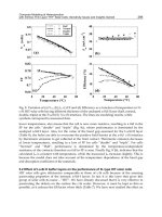
Fig. 5.1. Variation of solution pH with ammonia addition at 25 °C

NH
3
/NaCl
0.0 0.5 1.0 1.5 2.0 2.5 3.0 3.5 4.0
Sodium Removal %
0
10
20
30
40
Reject Brine

Synthetic Brine

Fig. 5.2. Variation of sodium removal with NH
3
/NaCl molar ratio at 20 °C
It is important to note that the stoichiometric amount of ammonia required by Reaction (5.1)
is one mole. However, in a real process excess ammonia may be needed for the reaction to
reach completion. An experimental evaluation of the effect of excess ammonia on the
removal of sodium at 20°C (El-Naas et al, 2010) indicated that the percent removal of
sodium increased with increasing the NH
3
/NaCl ratio, reaching a maximum at 3 as shown
in Figure 5.2. Similar experiments with synthetic brine solution, containing only NaCl in
distilled water, in this study and in a previous study (Jibril and Ibrahim, 2001) revealed that
the optimum sodium removal was achieved at a lower molar ratio (NH
3
/NaCl) of 2. In both
Desalination, Trends and Technologies

246
cases, the molar ratio is higher than that required stiochiometrically, which may be due to the
fact that the reaction was carried out in a semi-batch reactor, where the CO
2
gas leaving the
reactor stripped away some of the ammonia from the solution. This will not be the case for an
industrial process, where the reactor will be run in a continuous mode and the ammonia is
recycled within the system. As for the even higher molar ratio observed for the reject brine
(NH
3
/NaCl=3), it is believed to be due to the presence of other impurities in the brine.

Metal carbonates in the brine may compete for ammonia and reduce its availability for
reaction with CO
2
. Magnesium carbonate (MgCO
3
), which is always present in the reject
brine, consumes ammonia to form magnesium hydroxide and ammonium bicarbonate
according to the following reaction:
NH
3
+ MgCO
3
+ 2H
2
O → NH
4
HCO
3
+Mg(OH)
2
(5.7)
Thermodynamic analysis of Reaction (5.7) indicates that this reaction is spontaneous for
temperatures less than 22 °C. Thus one additional mole of ammonia is consumed by
Reaction (5.7) to form magnesium hydroxide. This was confirmed experimentally, where
milky colored turbidity was observed after mixing the reject brine with ammonium
hydroxide.
It is worth noting here that after treatment of the reject brine through reactions with carbon
dioxide, other ions such as Mg
+2
and Ca

+2
were significantly reduced at the end of the
experimental runs. In fact, Mg
+2
, Ca
+2
and Sr
+2
were reduced by more than 98%. Sodium
(Na
+
), which is the main focus of the treatment, was reduced by about 42% at the optimum
conditions. This low reduction in sodium, however, is believed to only represent the
conversion to insoluble sodium bicarbonate, which is removed by filtration. Since the
amount of sodium in the filtrate comes from NaCl and soluble NaHCO
3
, the true conversion
can not be easily determined, and it is expected to be much higher than the 42%.
Controlling the solubility of NaHCO
3,
therefore, is a crucial step in optimizing the Solavy
process for reject brine management.
5.4 Role of NaHCO
3
solubility
Sodium bicarbonate (NaHCO
3
) is an important intermediate product in the Solvay process
and its solubility plays an important role in the success of the process, since it determines
the amount of the solid product that can be removed by filtration. For the process to achieve

high conversion, the solubility of NaHCO
3
must be as low as possible. It is imperative,
therefore, to evaluate factors that can limit or reduce its solubility. At room temperature, the
solubility was determined experimentally to be about 9.75 g/100g and found to be
negatively affected by the presence of other intermediates and reactants in Reaction (5.1)
such as NaCl and NH
4
HCO
3
.
5.4.1 Effect of NaCl
The solubility of NaHCO
3
was found to decrease drastically with increasing the
concentration of NaCl in the solution, from 9.75 g/100g at 0wt% NaCl to 3.6 g/100g at
10wt% NaCl as Shown in Figure 5.3. This is attributed to the presence of the sodium ion
(Na
+
) in the aqueous solutions of both salts. In aqueous solutions, both sodium chloride and
sodium bicarbonate are present in their ionic format:
NaCl (a) ⇔ Na
+
+ Cl
-
(5.8)
Reject Brine Management

247
NaHCO

3
(a) ⇔ Na
+
+ HCO
3
-
(5.9)
One would expect that increasing the concentration of the sodium ion (Na
+
), by adding
more NaCl into the solution, would force the equilibrium of Reaction (5.9) to the left and
hence reduce the solubility of NaHCO
3
. The solubility of NaCl in water at 25 °C is about 36
g/100g, which is almost four times that of NaHCO
3
. The reduction in NaHCO
3
solubility
with the presence of NaCl (Figure 5.3) seems to follow an exponential decay (y = 9.7e-
0.095x
).
According to this relation, the solubility of NaHCO
3
in a saturated NaCl solution will
diminish to merely 0.3 g/100g. This highlights the necessity for using saturated brine in the
Solvay process. It is to optimize the precipitation of NaHCO
3
by minimizing its solubility.
NaCl Concentration (Wt.%)

012345678910
NaHCO
3
Solubility (Wt%)
0
2
4
6
8
10
12
Y= 9.7 e
-0.095X

Fig. 5.3. Effect of NaCl on the solubility of NaHCO
3
at 25 °C
5.4.2 Effect of ammonium bicarbonate
Ammonium bicarbonate is another important intermediate in the formation of sodium
bicarbonate according to Reactions 5.4 and 5.5. Its effect on the solubility of NaHCO
3
was
evaluated for two aqueous solutions, containing 4% and 8% sodium chloride. The results are
shown in Figure 5.4. Clearly, raising the concentration of ammonium bicarbonate seems to
have a detrimental effect on the solubility of NaHCO
3
. The rate of reduction in the solubility
seems to be higher (about 33%) for the solution containing 8% NaCl. One may use similar
argument to that used in the case of NaCl to explain this decline in the solubility. In this
case, increasing the concentration of (HCO

3
-
) by adding more ammonium bicarbonate
would force the equilibrium in Reaction (5.11) below to the left and thus lower the solubility
of NaHCO
3
.
NH
4
HCO
3
(a) ⇔ NH4
+
+ HCO
3
-
(5.10)
NaHCO
3
(a) ⇔ Na
+
+ HCO
3
-
(5.11)
The experimental results (Figure 5.4) indicate that for an aqueous solution containing 8%
NaCl, the solubility of NaHCO
3
can be reduced to 0.0 g/100g with the addition of about
13wt% ammonium bicarbonate, which can definitely have significant effect on the

possibility of using the Solvay process for reject brine management.
Desalination, Trends and Technologies

248

NH
4
HCO
3
(W t% )
01234567891011
NaHCO
3
Solubility (W t% )
0
1
2
3
4
5
6
7
8
NaCl = 4%
NaCl = 8%


Fig. 5.4. Effect of NH
4
HCO

3
on the solubility of NaHCO
3
at 25 °C
Ammonium chloride (NH
4
Cl) is another byproduct formed in the Solvay process. Its effect
on the solubility of NaHCO
3
was assessed in about the same way as that used with
ammonium bicarbonate. The results, however, were not similar. The solubility of sodium
bicarbonate does not seem to be affected by the presence of NH
4
Cl regardless of the
concentration of NaCl. This may be attributed to the fact that ammonium chloride is not
involved in the formation of sodium bicarbonate and does not have any common ions with
NaHCO
3
; therefore, it does not affect its ionic equilibrium at these concentrations and
temperature.
6. Industrial applications and CO
2
Capture
Application of the Solvay process for reject brine management has another important
feature, which is the potential for carbon capture and storage (CCS). The process can be
utilized for the removal of CO
2
from flue gases or for the sweetening of natural gas. Carbon
dioxide is a major contributor to global warming and believed to have the greatest adverse
impact on the observed greenhouse effect causing approximately 55% of global warming.

The most common approach to CCS involves capturing CO
2
and then injecting it into rock
layers in depleted or near-depleted oil and gas fields. The aim, off course, is to store the CO
2

and at the same time utilize it for Enhanced Oil Recovery (EOR). Although this option has
gained the support of many industrialized and oil producing countries alike, it is not really
problem-free and its long term effects are not yet known (El-Naas, 2008). Under typical
storage conditions (1000 m below the surface), the density of CO
2
phase is approximately
two-thirds that of the underground brine, which provides the driving force for escape
(Bryant, 2007). Gradual seepage of CO
2
into the atmosphere may not pose much harm to
human life, but it will certainly defeat the purpose of CCS.
Carbon dioxide reactions with ammoniated brine can offer a dual-purpose approach for the
management of reject brine and capture of CO
2
. The main unit of the process is the contact
Reject Brine Management

249
reactor, where the flue gases are contacted with the ammoniated reject brine. Other units
include the ammoniating tank, where the high salinity water is mixed with ammonia gas;
the ammonia recovery reactor, where the ammonia is recovered through reaction with
calcium hydroxide; and a filter to separate the precipitated sodium bicarbonate from the rest
of the solution. A schematic diagram of the process is shown in Figure 5.5. The carbon
dioxide captured through this process is stored in the form of sodium bicarbonate.

NH3
Flue
Gases
Ca(OH)
2
Contact
Reactor
Reject
Brine
Solid
Product
Low Salinity
Water
Filter
CO
2
Free
Flue
Gases


Fig. 5.5. A schematic diagram of a reject brine management process
The effectiveness of capturing CO
2
through the reaction with ammoniated brine was
assessed experimentally. A gas mixture containing 10% CO
2

in methane was bubbled
through one liter of ammoniated brine in three semi-batch bubble columns in series. The gas
effluent of the first column was bubbled through the second and then the third. Half of the
ammoniated brine was placed in the first column while the other half was divided equally
between the other two columns. The total gas flow rate was controlled at 47 liter/hr using
two mass flow controllers. The concentration of carbon dioxide and methane in the effluent
gas stream were analyzed using a dual channel CO
2
and CH
4
infrared analyzer.
The experimental results for the CO
2
percent removal through the reaction with
ammoniated reject brine solution are presented in Figure 5.6. It is evident that there is a
considerable reduction in the CO
2
concentration in the effluent stream with 100% removal in
the first two hours and more than 80% removal for the first five hours of run time. It is
noticeable, nonetheless, that the percent removal is declining with time due to the
consumption of the main reactants in the solution. Since the reactors were operated in the
semi-batch mode, where only gases enter and leave the system, the other reactants in the
ammoniated brine (NH
3
and NaCl) were consumed with time and hence less CO
2
was
removed with time as shown in the figure. Although these results confirm the technical
viability of the process for CO
2

capture and reduction of the reject brine salinity, more
research is still needed to optimize the reactor design for continuous operation. An
industrial process can be developed to offer an effective solution for the two major
environmental challenges: reject brine management and CO
2
capture.
Desalination, Trends and Technologies

250
Time (h)
0 2 4 6 8 1012141618202224
CO
2
Removal (% )
0
10
20
30
40
50
60
70
80
90
100

Fig. 5.6. CO
2
removal from a gas mixture containing 10% CO
2

in methane through reaction
with ammoniated brine at 20 °C in a semi-batch three bubble columns in series.
7. Conclusions
Reject brine management represents a major environmental and economical challenge for
most desalination plants. The current options for brine management are rather limited and
have not achieved a practical solution to this environmental challenge. A new approach
that involves reactions with CO
2
in the presence of ammonia has proven to be effective in
reject brine management and capture of CO
2
.
8. References
Ahmed, M., W. H. Shayya, D. Hoey and J. Al-Handaly, “Brine disposal from reverse
osmosis desalination plants in Oman and United Arab Emirates,” Desalination 133,
135-147 (2001).
Ahmed, M., W. H. Shayya, D. Hoey, A. Maendran, R. Morris and J. Al-Handaly, “Use of
evaporation ponds for brine disposal in desalination plants,” Desalination, 130,
155-168 (2000).
Al-Faifi , H., A.M. Al-Omran, M. Nadeem, A. El-Eter , H.A. Khater , S.E. El-Maghraby, Soil
deterioration as influenced by land disposal of reject brine from Salbukh water
desalination plant at Riyadh, Saudi Arabia, Desalination 250 (2010) 479–484.
Yeh, A. C. and H. Bai, "Comparison of ammonia and monoethanolamine solvents to reduce
CO greenhouse gas emissions", The Science of the Total Environment 228 (1999)
121-133.
El-Naas, M. H, A different approach for Carbon Capture and Storage (CCS), Research
Journal of Chemistry and Environment, Volume 12, Issue 2, June 2008, Pages 3-4.
El-Naas, M. H., A. H. Al-Marzouqi, O. Chaalal, “A combined approach for the management
of desalination reject brine and capture of CO
2

”, Desalination 251 (2010) 70–74.
Reject Brine Management

251
Gilron, J., Y. Folkman, R. Savliev, M. Waisman, O. Kedem, "WAIV - wind aided intensified
evaporation for reduction of desalination brine volume", Desalination, 158 (2003)
205.
Glater, J. and Y. Cohen, Brine disposal from land based membrane desalination plants a
critical assessment, a report prepared for the Metropolitan Water District of
Southern California, July 2003.
Hoffman, D., J.D. Rhodas, J. Letey and F. Sheng, Salinity management. In: G.J. Hoffman,
T.A. Howell and K.H. Soloman, Editors, Management of Farm Irrigation Systems,
American Society of Agricultural Engineers, New York (1990), pp. 667–715.
Jibril, B. and A. Ibrahim, "Chemical Conversions of salt concentrates from desalination
plants" Desalination, 139 (2001) 287.
Khordagui, H.,Environmental aspects of brine reject from desalination industry in the
SCWA region. ESCWA, Beirut, 1997.
Kostick, D., "Soda Ash", chapter in Minerals Yearbook, United States Geological Survey
(2005).
Lattemann, S., T. Höpner, Environmental impact and impact assessment of seawater
desalination, Desalination 220 (2008) 1–15.
Maas, E.V., Crop salt tolerance. In: K.K. Tanji, Editor, Agricultural Salinity Assessment and
Management, Amercian Socity of Civil Enginers, New York (1990), pp. 262–303.
Mickley, M. C., Membrane Concentrate Disposal: Practice and Regulation,”, Prepared for
the U.S. Department of the Interior, Bureau of Reclamation, Technical Service
Center, Water Treatment Engineering and Research Group, September 2001.
Mickley, M., Membrane Concentrate Disposal: Practices and Regulation, Second Edition.
U.S. Department of the Interior, Bureau of Reclamation, Technical Service Center,
Water Treatment Engineering and Research Group, April 2006.
Mickley, M., R. Hamilton, L. Gallegos and J. Truesdall, Membrane concentration disposal,

American Water Works Association Research Foundation, Denver, Colorado, 1993.
Mohamed, A.M.O., M. Maraqa and J. Al Handhaly, Impact of land disposal of reject brine
from desalination plants on soil and groundwater, Desalination 182 (2005), pp. 411–
433.
Rao, N.S., R.T.N. Venkateswara, G.B. Rao and K.V.G. Rao, Impact of reject water from the
desalination plants on ground water quality, Desalination 78 (1990), pp. 429–437.
Rhee, S-W, D. D. Reible and W. D. Constant, “Stochastic modeling of flow and transport in
deep-well injection disposal systems,” J. Hazardous Materials, 34, 313-333 (1993).
Roine, A., “Outokumpu HSC Chemistry for Windows”, Ver. 6.12, User’s guide, Outokumpu
Research Oy, 2007.
Sadhwani, J. J., J. M. Veza, C. Santana, Case studies on environmental impact of seawater
desalination, Desalination 185 (2005) 1–8.
Sánchez-Lizaso, J. L, J. Romero, J. Ruiz, E. Gacia, J. Buceta, O. Invers, Y. Torquemada, J.
Mas, A.Ruiz-Mateoe, M. Manzanera, Salinity tolerance of the Mediterranean
seagrass Posidonia oceanica: recommendations to minimize the impact of brine
discharges from desalination plants, Desalination 221 (2008) 602–607.
Saripalli, K. P., M. M. Sharma and S. L. Bryant, “Modeling Injection Well Performance
During Deep-Well Injection of Liquid Wastes,” J. Hydrology, 227, 41-55 (2000).
Desalination, Trends and Technologies

252
Skehan, S and P. J. Kwiatkowski, “Concentrate Disposal via injection wells – permitting and
design considerations,” Florida Water Resources J., May 2000, 19-22.
12
DOE Method for
Optimizing Desalination Systems
Amin Behzadmehr
Mechanical Engineering Department, University of Sistan and Baluchestan
I.R.Iran
1. Introduction

Fresh water production is one of the main concerns in the new century. Population grows
fast and potable water resources are decreased. In the other hand energy crises would also
be another issue that must be well addressed by the politicians and also scientists.
Developing desalination plant with using renewable energy (particularly solar energy) is
one of the important options to overcome these concerns. Thus many researchers have been
working on different desalination plants to find the best conditions and to realize the most
efficient performances for different cycles. Different approaches have been used to achieve
the most efficient conditions or to find the optimum operation and design conditions. Some
of the researchers used parametric study approach while many other adopted different
conventional optimization algorithms for these tasks. The algorithms such as gradient based
algorithm, genetic algorithm, search and pattern algorithm and neural network method
have been used in the field of desalination. For instance; Ophir and Lokiec (2005) described
the design principles of a MED plant and various energy considerations that result in an
economical MED process and plant. Kamali and Mohebbinia (2007) showed that parametric
study as one of the optimization methods on thermo-hydraulic data strongly helps to
increase GOR value inside MED-TVC systems. Shamel and Chung (2006) used parametric
study to find the optimum condition of a Reverse Osmosis (RO) system for sea water
desalination. Metaiche et al (2008) developed optimization software, Desaltop, for RO
system for water desalination. They used genetic algorithm to find suitable operating
parameters and also to find appropriate type of membrane. Al-Shayji (1998) used neural
network method for optimization of large-scale commercial desalination plants. Djebedjian
et al. (2008) used genetic algorithm for optimization of a reverse osmosis desalination
system. Mussati et al. (2003) used an evolutionary algorithm for the optimization of Multi
Stage Flash (MSF) system. Finding the optimum conditions is a major challenge on the
desalination plant studies. The plant performance depends on several different variables
and constraints that need exhausting efforts to find the optimum conditions.
This chapter introduces Design of Experiment (DOE) method as a statistical tool for
optimization of desalination systems. Thus two different desalination plants; Multi-Effect
Desalination (MED) system and solar desalination using humidification–dehumidification
cycle (SDHD) have been considered to show the ability of DOE method for optimizing such

systems. These both desalination plants could use the low graded heating energy sources
Desalination, Trends and Technologies

254
such as solar energy. Thus it is very important to know the best thermodynamic conditions
(variables) for which the desired objectives (objective functions) could be attained based on
the technological and economical constraints. General perspective of effects of these
thermodynamic conditions at different points of the plant on the rate of fresh water
production and also the quantity and quality of heating energy sources would be very
important and very useful for a plant designer. DOE method could show the optimal
thermodynamic conditions of these systems.
Thus, first DOE method is briefly presented and then this method is adopted to investigate
the MED plant and a solar desalination using humidification-dehumidification system.
2. Principles of Design of Experiments
Design of Experiment (DOE) is a statistical approach that could clearly show how much
several parameters of a system as well as their interactions are important on the plant
output and how these parameters could affect the objective function. DOE Method is
capable to investigate simultaneously the effects of multiple parameters on an output
variable (response). To illustrate statistically reasonable conclusions from the experiment, it
is necessary to integrate an efficient statistical method into the methodology of experimental
design. In the context of DOE in designing, one may encounter two types of plant variables
or factors: qualitative and quantitative factors. For quantitative factors, the range of settings
must be decided by designer. For instance, pressure, temperature or heat transfer surface are
examples of quantitative factors. Qualitative factors are discrete in nature. For example,
types of materials, nature of heating source, and types of equipments are examples of
qualitative factors. A factor may take different levels, depending on the character of the
factor- quantitative or qualitative. In general, compared to a quantitative factor, more levels
are required by a qualitative factor. “Level” in this chapter refers to a specified value or
setting of the factor that would be examined in the plant experiment. For instance, if the
experiment is to be performed at three different pressures or using three different types of

preheaters, then it could be said pressure or preheater has three levels. Three fundamental
approaches on experimental design are replication, blocking, and randomization. The first
two help to increase precision in the experiment; the last one is used to reduce bias. These
three principles of experimental design can be used by industrial designer to improve the
efficiency and performance of a product (see Behzadmehr et al. 2006a, 2006b). In addition
these principles of experimental design are applied to decrease or even remove
experimental bias. It should be mentioned that the large experimental bias could result in
wrong optimal conditions or sometimes it could mask the effect of the really significant
factors. This could cost lost of a primary factor for plant improvement.
Details and mathematical concepts of DOE are out of this chapter objective. The interested
reader would find complete description of this method in the relevant text books such as
Antony (2003) or book by Montogomery (2001).
3. Case I) Thermodynamic optimization of MED plant using DOE method
The multi-effect desalination (MED) plant is one of the most efficient thermal desalination
processes currently in use. Development of MED in the last few years has brought this
process to the point of competing economically and technically with the multi-stage flashing
(MSF) process. MED process is based on the pressure reduction of water in each effect.
DOE Method for Optimizing Desalination Systems

255
Many researchers have studied this process. Among them Sharmmiri and Safar (1999)
discussed the general aspects of some commercial MED plants and also some of their
specifications such as type of plant configuration, gain output ratio, number of effects,
operating temperature and the construction material for the evaporator, condenser and
preheaters. Ophir and Lokiec (2005) described the design principles of a MED plant and
various energy considerations that result an economical MED process and plant. They also
provided an overview of various cases of waste heat utilization, and cogeneration MED
plants operating. Aybar (2004) considered a multi effect desalination system using waste
heat of a power plant as energy source. A simple thermodynamic analysis of the system was
performed with using energy and mass balance equations. Khademi et al. (2009) focused on

the development of a steady-state model for the multi-effect evaporator desalination system.
Hatzikioseyian et al. (2003) reviewed and developed a simulation program based on design
parameters of the plant. They used mass and energy balance through each effect of the MED
unit to predict the performance of the unit in terms of energy requirements. Kamali and
Mohebbinia (2007) showed that parametric study as one of the optimization methods on
thermo-hydraulic data strongly helps to increase GOR value inside MED-TVC systems. El-
Nashar (2000) simulated part-load performance of small vertically stacked MED plants of
the HTTF type using hot water as source of energy. Their model was validated with the
experimental data obtained from an existing plant in operation. Narmine and El-Fiqi (2003)
described a steady state mathematical model to analyze both multi-stage and multi-effect
desalination systems. Relationships among the parameters which controlling the cost of
fresh water production to the other operating and design parameters were presented.
Parameters include plant performance ratio (PR), specific flow rate of brine, top brine
temperature, and specific heat transfer area.
Here as an example the sensitivity of some important parameters on the minimum and
maximum distilled water production is analyzed. Therefore the effects of feed water flow
rate and its temperature, the number of effects, preheater temperature difference
(performance of each preheater), and minimum pressure (at the end stage) are studied. Thus
the mass, energy and salinity balance equations are solved for each effect to calculate
temperature, pressure salinity of brine, enthalpies of outlet at each effect and mass flow rate
of distilled water. For thermodynamic analysis and plant optimization, design of experiment
method (DOE) is used to find the effective parameters on the minimum and maximum fresh
water production.
3.1 Plant description
The multi effect desalination is an important process that has been used for desalination
particularly in large scale plants. This method reduces considerably the production cost
(Ophir and Lokiec 2005). The main parts of MED plant are: 1-Condenser, 2-Evaporator, 3-
Collector (thermal source) and 4-Preheaters (heat exchanger). Each effect except the last one
includes a preheater and an evaporator. The hot water circulates between the top effect
evaporator and solar collector to supply thermal energy to the evaporator in the form of hot

water flowing through the tube bundle of the first effect. The preheated sea water is sprayed
on the tube bundle of first evaporator and vapour is generated. In the other effects, vapour
is generated by both boiling and flashing processes. Pressure reduces on each effect to
produce more vapours. Figure 1 shows a vertical configuration of MED plant.
Desalination, Trends and Technologies

256

Fig. 1. Schematic diagram of MED plant
DOE Method for Optimizing Desalination Systems

257
3.2 Mathematical modeling
A schematic of main multi effect desalination plant’s parts is shown in Fig. 2. As seen in Fig.
2a the mass, energy and salinity balance equations for evaporator at the first effect (top
effect) are as follow:
Mass balance equation:

(1)m(1)mm
v
bf

+=
(1)
Balance of salinity:

)1(X)1(mXm
bb
sw
f


=
(2)
Balance of energy:

)1(h)1(m)1(h)1(m)1(hmQ
vv
bbfof


+=+
(3)
It is well known that the enthalpy of brine in each effect could be considered a function of
salinity and temperature while the enthalpy of saturated vapour is only a function of
temperature. Thus these equations are used to find temperature and salinity relationship. As
shown schematically in Fig. 2b, preheaters consider being shell and tube heat exchanger.
The mass and energy balance for all preheaters are as follow:
Mass balance equation

)i(m)i(m
v
d

=
(4)
Energy balance equation:

)i(h)i(m)i(hm)i(hm)i(h)i(m
vv
fiffofdd


+=+
(5)
Figure 2c shows the evaporator of the second effect. The mass, energy and salinity balance
equations for this part are:
Mass balance equation:

)1(m)1(m,)2(m)2(m)1(m
d
oev
bb

=
+
=
(6)
Salinity balance equation:

)2(X)2(m)1(X)1(m
bbbb

=
(7)
Energy balance equation:

)2(h)2(m)2(h)2(m)2(h)2(m)1(h)1(m)1(h)1(m
oeoevv
bbddbb

+

+
=
+
(8)
Energy balance equation:

)2(h)2(m)2(h)2(m)2(h)2(m)1(h)1(m)1(h)1(m
oeoevv
bbddbb

+
+
=
+
(8)
Other evaporators are fed from both outlet of the previous evaporator and from the exit of
distilled water side (mixture of vapour and condensed water) of the previous preheater.
This is shown in Fig. 2d. The balance equations can be written as follows:
Desalination, Trends and Technologies

258
Mass balance equation:

)i(m)i(m,)i(m)i(m)1i(m
ieoev
bb

=
+
=

−
(9)
Balance of salinity:

)i(X)i(m)1i(X)1i(m
bbbb

=
−
−
(10)
Balance of energy equation:

)i(h)i(m)i(h)i(m)i(h)i(m)i(h)i(m)1i(h)1i(m
oeoevv
bb
ieie
bb

+
+
=
+
−
−
(11)
Where:

n, ,4,3i,)1i(m)1i(m)i(m
d

oeie
=
−
+
−
=

(12)

n, ,4,3i,
)1i(m)1i(m
)1i(h)1i(m)1i(h)1i(m
)i(h
d
oe
dd
oeoe
ie
=
−+−
−
−
+
−
−
=


(13)
The last effect of MED plant just includes a condenser (see Fig. 2e).

Fig. 2. Control volume of MED parts
The mass and energy balance in this stage are:
Mass balance equation:
DOE Method for Optimizing Desalination Systems

259

dis
icon
mm

=
(14)
Energy balance equation:

disdisfif
swswiconicon
hm)n(hmhmhm

+=+
(15)
Where:

)n(m)n(mm
d
oeicon

+

=
(16)

)n(m)n(m
)n(h)n(m)n(h)n(m
h
d
oe
dd
oeoe
icon


+
+
=
(17)
The equations (1)-(17) are simultaneously solved to predict the thermodynamic properties of
water and steam (temperature, pressure, enthalpy and salinity) at each part. The
thermodynamic properties of distilled water, water vapour and brine are calculated for
known parameters and P
out
in the simulation code. Since these parameters have been
specified in the simulation code, the input heating energy (
Q

) must be limited to a particular
range based on these parameters in order to achieve the balanced thermodynamic
conditions at all parts of MED plant. Therefore for given input parameters minimum and
maximum values for the heating energy is calculated for which equations (1)-(17) would be

thermodynamically balanced with real physical conditions. More details of numerical
procedure and validation could be found in the work by Kazemian et al. (2010).
3.3 Results and discussions
The effects of different parameters such as feed water flow rate, temperature of feed water,
number of effects, temperature difference of preheaters and output pressure on the rate of
fresh water production have been studied. Therefore to be more efficient the test conditions
are design based on the method of design of experiment (DOE). DOE is performed on k
parameters at two or more than two levels to understand their direct effects and also their
interactions on the desired responses (Montogomery 2001). First a 2
k
factorial design is
chosen to construct the tests table. Five parameters are selected to study their effects on the
minimum and maximum distilled water. These parameters are: feed water flow rate (A),
temperature of feed water (B), number of effects (C), temperature difference of preheater (D)
and output pressure (E).

Factors Parameters Level 1 Level 2 Level 3
A
Feed water ( s/kg )
30 60 90
B Temperature of seawater (ºC) 25 30 32.5
C Number of effects 12 15 18
D Temperature difference of each pre-heater (
o
C) 1 3 5
E Out-put pressure (MPa) 0.003 .004 0.005
Table 1. Parameters and their three levels value for
3
k
factorial model of minimum distillate

Desalination, Trends and Technologies

260
Source Sum of Squares df Mean Square F Value p-value
Model 2076.82 20 103.841 846.4712 < 0.0001 Significant
A-
f
m
597.2135 1 597.2135 4868.251 < 0.0001 Significant
B-
sw
T

3.868855 1 3.868855 31.5374 0.0002 Significant
C-n 549.1412 1 549.1412 4476.385 < 0.0001 Significant
D-
p
r
TΔ

539.6624 1 539.6624 4399.118 < 0.0001 Significant
E-
out
P
42.44459 1 42.44459 345.9918 < 0.0001 Significant
AB 0.617234 1 0.617234 5.031455 0.0464 Significant
AC 87.78436 1 87.78436 715.5839 < 0.0001 Significant
AD 86.38329 1 86.38329 704.1629 < 0.0001 Significant
AE 6.796065 1 6.796065 55.39888 < 0.0001 Significant
BC 1.162114 1 1.162114 9.473101 0.0105 Significant

BD 0.561878 1 0.561878 4.580208 0.0556 Non significant
BE 4.281921 1 4.281921 34.90455 0.0001 Significant
CD 126.191 1 126.191 1028.66 < 0.0001 Significant
CE 5.539345 1 5.539345 45.15458 < 0.0001 Significant
DE 1.563831 1 1.563831 12.74774 0.0044 Significant
ABE 0.684065 1 0.684065 5.576231 0.0377 Significant
ACD 20.19142 1 20.19142 164.5926 < 0.0001 Significant
ACE 0.884603 1 0.884603 7.210942 0.0212 Significant
BCD 0.431494 1 0.431494 3.517369 0.0875 Non significant
BDE 1.416334 1 1.416334 11.5454 0.0060 Significant
Table 2. analysis variance of
3
k
factorial model for minimum distillate
A 2
k
factorial with two levels for the minimum distilled water has been performed to see if
there are any non significant parameters. It should be mentioned that the signification of the
parameters are quantified by the p-value, a p-value less than 0.05 indicates significance
(Montogomery 2001) and are specified as significant parameter. The results show that the
effects of these parameters on the minimum distilled water are significant (see Fig. 3).


Fig. 3. Response of first DOE for minimum distilled water
DOE Method for Optimizing Desalination Systems

261
Thus in order to have more accuracy a new DOE with three levels is performed to study the
effects of these parameters on the minimum distilled water a 3
k

factorial test table is
designed which is shown in table 1.
Therefore 243 ( 3
5
) tests have been executed to find the response of the objective function
(minimum distilled water) on the variations of these parameters. Analysis variance of the 3
k

factorial tests is shown in table 2. Then a regression has been performed on the results of
factorial to show and also to predict the effects of these parameters on the minimum water
distilled. Equation (19) is the regression function estimated from DOE analysis of minimum
amount of distilled water.

outproutprsw
outswprsw
4
out
f
outpr
f
pr
f
4
t
ousw
f
prsw
f
4
sw

f
5
outpr
outproutswprsw
sw
3
out
f
pr
f
4
f
3
sw
f
3
out
prsw
f
min
d
PTn57852.1PTT71972.24
PnT18593.0TnT1056007.9Pnm19816.0
PTm28864.0Tnm1014699.5PTm34827.0
TTm1019483.1nTm1071863.1PT91251.749
Pn34805.26Tn049661.0PT27274.95TT090929.0
nT1014011.3Pm08346.6T
m1039631.1
nm10177766.1Tm1073109.1P42454.3042
T64044.2n014194.0T35466.0m023307.001593.11-)m(

×Δ×+×Δ×+
××+Δ×××−××+
×Δ×+Δ×××+××−
Δ×××−×××+×Δ−
×−Δ×+×−Δ×−
××+×
+Δ××+
××−××++
Δ+++−=
−
−
−−
−−
−−

(19)
For given values of the parameters the prediction contours of minimum water distilled can
be plotted by this equation. In order to see the precision of the predicted results by these
contours, comparisons are done with the results obtained directly from the simulation code.
As seen in table 3, within the range of performed tests, these results are very close while out
of the range of executed tests the concordance between the results is acceptable (6.59%).

Prediction Actual Error%
In the range 8.958 8.896 0.69
Out of the
range
34.398 36.8249 6.59
Table 3. Predicted error for the minimum distilled water
The same approach is also adopted for the maximum distilled water. The results of 2
k

factorial tests for the maximum amount of distilled water shows that the effect of parameter
B (T
sw
) on the maximum amount of distilled water is negligible (see in Fig. 4). Thus another
tests routine with factorial is performed. The parameters and their levels (three for each)
are shown in table 4. The tests table for analysis of variance of maximum amount of distilled
water consists of 81 tests (3
4
) which is presented in table 5.

Factors Parameters Level 1 Level 2 Level 3
A Feed water (kg/s) 30 50 70
B Number of effects 12 15 18
C Temperature difference of each pre-heater (
o
C) 2 3 4
D Output pressure (MPa) 0.003 .0045 0.006
Table 4. Parameters and their three levels value for 3
k
factorial model of maximum distillate
Desalination, Trends and Technologies

262
Source Sum of Squares df Mean Square F Value
p-value
Prob > F

Model 4974.632 11 452.2393 3444.212 < 0.0001 significant
A-mf 2447.064 1 2447.064 18636.61 < 0.0001 Significant

B-n 661.6533 1 661.6533 5039.089 < 0.0001 Significant
C-deltpr 1583.357 1 1583.357 12058.69 < 0.0001 Significant
D-Pout 0.278922 1 0.278922 2.124243 0.1495 Non- significant
AB 70.48853 1 70.48853 536.834 < 0.0001 Significant
AC 168.8939 1 168.8939 1286.28 < 0.0001 Significant
AD 0.03011 1 0.03011 0.229317 0.6335 Non- significant
BC 29.61552 1 29.61552 225.549 < 0.0001 Significant
CD 9.119239 1 9.119239 69.45126 < 0.0001 Significant
ABC 3.161682 1 3.161682 24.07907 < 0.0001 Significant
ACD 0.970699 1 0.970699 7.392755 0.0083 Significant
Table 5. analysis variance of 3
k
factorial model for maximum distilled water
The estimated function resulted from DOE analysis for maximum distilled water is as
follow:

outpr
f
pr
f
3
outprsw
4
out
f
pr
ff
3
out
pr

43
f
3
max
d
PTm70371.6Tnm1004926.6
PT34856.0nT1028832.1Pm07516.21
Tm012606.0nm1017374.5P7575.0
T1024331.3n1011264.1m02892.01098114.9)m(
×Δ×+Δ×××+
×Δ+××−×−
Δ×−××+−
Δ×+×++×−=
−
−
−
−−−

(20)


Fig. 4. Response of first DOE for maximum distilled water
To show the precision of this equation comparisons are done with the direct results of the
simulation code. As seen in table 6 within the range of performed tests, the results are
very close while at the out of range the concordance between the results is acceptable
(4.33%).
DOE Method for Optimizing Desalination Systems

263
Error% actual Prediction

1.27 13.5522 13.724 In the range
4.33 44.9896 43.0413 Out of the range
Table 6. Predicted error for maximum distilled water
Thus at this step the contours for prediction of minimum and maximum distilled water
could be presented and discussed.
As mentioned the regression functions are obtained by using the responses of the
parameters on the objective function. These functions are composed of the effective
parameters and their interactions. The contours of responses on each parameter could be
plotted using these equations. These contours are an excellent tools to show the effect of
each parameter rather than calculating by the simulation code.
Several contours are shown in Figs 5-10 (these results were presented by Kazemian et al.
2010). It is shown that the amount of feed water mass flow rate has a significant effect on
increasing the amount of minimum distilled water. As seen in Fig. 5, for a given feed water
mass flow rate, increasing the temperature of the inlet feed water slightly augments the
amount of minimum distilled water.
There are two parallel phenomena to increase the amount of minimum distilled water by
increasing the numbers of effects (see Fig. 6). The top brine temperature is increased by
increasing the effects, so the salt concentration in the first effect is increased and more vapours
is produced. On the other hand, the pressure and temperature differences of effects are
decreased by increasing the effects. Therefore the salt concentration differences at each effect
would be decreased and the amount of distilled water would be increased. The influence of
increasing temperature difference of preheaters on the minimum distilled water production is
fairly the same as the one that was seen by increasing the numbers of effects (Fig. 7).

Fig. 5. Contour of minimum distilled water for N=15, ΔT
pr
=3
o
C, P

out
=0.004MPa