Digital Filters Part 3 potx
Bạn đang xem bản rút gọn của tài liệu. Xem và tải ngay bản đầy đủ của tài liệu tại đây (1.01 MB, 20 trang )
The application of spectral representations in coordinates
of complex frequency for digital lter analysis and synthesis 31
The model (1) also makes it possible to describe the majority of impulse signals, which are
widely applicable in radio engineering. Examples of some impulse signals are shown it the
Table 2. Therefore, the generalized mathematical model (1) enables to describe a big variety
of semi-infinite or finite signals.
As it is shown below, the compound finite signal representations in the form of the set of
damped oscillatory components significantly simplifies the problem solving of the signal
passage analysis through the frequency filters, by using the analysis methods based on signal
and filter spectral representations in complex frequency coordinates (Mokeev, 2007, 2008b).
2.2 Mathematical description of filters
Analysis and synthesis of filters of digital automation and measurement devices are
primarily carried out for analog filter-prototypes. The transition to digital filters is
implemented by using the known synthesis methods. However, this method can only be
applied for IIR filters, as a pure analog FIR filter does not exist because of complications of
its realization. Nevertheless, implementation of this type of analog filters is rational
exclusively as they are considered “perfect” filters for analog signal processing and as filter-
prototypes for digital FIR filters (Mokeev, 2007, 2008b).
When solving problems of digital filters analysis and synthesis, one will not take into
account the AD converter errors, including the errors due to signal amplitude quantization.
This gives the opportunity to use simpler discrete models instead of digital signal and filter
models (Ifeachor, 2002, Smith, 2002). These types of errors are only taken into consideration
during the final design phase of digital filters. In case of DSP with high digit capacity, these
types of errors are not taken into account at all.
The mathematical description of analog filter-prototypes and digital filters can be expressed
with the following generalized forms of impulse functions:
T 'T
( )
t
t
g t e e
Q
q
C T
G G ,
( ) Re ( )
g
t
g
t ,
(4)
T 'T
( ) , ,g k Z k Z kG q G Q C N ,
( ) Re ( )
g
k
g
k .
(5)
Therefore, for analog and digital filter description it is sufficient to use vectors of complex
amplitudes of two parts of complex function:
m
j
m m
M
M
G k eG and
' '
m m
T
m m
M
M
G G eG , vector of complex frequencies
m m m
M
M
jwq
and vectors
m
M
TT и
m
M
NN , which define the duration
(length) of the filter pulse function components;
diagQ q
– is a square matrix M×M with
the vector
q
on the main diagonal.
Adhering to the mathematical description of the FIR filter impulse function mentioned
above (4), the IIR filter impulse functions are a special case of analogous functions of FIR
filters at
'
G 0 .
Recording the mathematical description of filters in such a complex form has advantages:
firstly, the expression density, and secondly, correlation to two filters at the same time,
which allows for ensured calculation of instant spectral density module and phase on given
complex frequency (Smith, 2002).
The transfer function of the filter (4) with the complex coefficients is
T 'T
1 1
( )
m
pT
m m
M
M
K p e
p p
G G ,
(6)
The transfer function ( )K p is an expression of the complex impulse function (6), therefore it
has along with the complex variable
p
complex coefficients, defined by the vectors
,G
'
G and q . A filter with the transfer function ( )K p correlates with two ordinary filters,
which transfer functions are
Re ( )K
p
and
Im ( )K
p
. In this case the extraction of the real
and imaginary parts of
( )K p can be applied only to complex coefficients of the transfer
function and has no relevance for the complex variable
p
.
As it appears from the input signal models (1) and filter impulse functions (4), there is a
similarity between their expressions of time and frequency domains. Filter impulse
functions based on the model (4) may have a compound form, including the analogous ones
referred to above in Tables 1 and 2.
The similarity of mathematical signal and filter expressions: firstly, allow to use one
compact form for their expression as a set of complex amplitudes, complex frequencies and
temporary parameters. Secondly, it significantly simplifies solving problems of
mathematical simulation and frequency filter analysis.
The digital filter description (5) can be considered as a discretization result of analog filter
impulse function (4). Another known transition (synthesis) methods can be also applied, if
they are revised for use with analogue filters-prototypes with a finite-impulse response
(Mokeev, 2008b).
2.3 Methods of the transition from an analog FIR filter to a digital filter
The mathematical description of digital FIR filters at 1M is given in the Table 3, these
filters were obtained on the basis of the analog FIR filter (item 0) by use of three transformed
known synthesis methods: the discrete sampling method of the differential equation (item
1), as well as the method of invariant impulse responses (item 2) and the method of bilinear
transformation (item 3).
№ Differential or difference equation Impulse function Transfer or system function
0.
'
1 1 1 1
( )
( ) ( ) ( )
dy t
y t G x t G x t
dt
1 11
( )
'
1 1
( )
t
t
g t G e G e
1
'
1 1
1
1
( )
p
K p G G e
p
1.
1
1 1 2k k k k N
y y G x G x
1
11 1 11 1
11
k N
k
k
g k G z G z
1
11
1 2
11
( )
N
k z
K z G G z
z z
2.
1
0 1 2k k k k N
y a y G x G x
1
12 1 1 1
1
k N
k
k
g k G z G z
1
12
1 2
1
( )
N
k z
K z G G z
z z
3. -
-
1
13 1 2
13
1
( )
N
z
K z k G G z
z z
Table 3. Methods of the transition from an analog FIR filter to a digital FIR filter
Note: The double subscripts are given for the parameters that do not coincide. The second
number means the sequence number of the transition method.
1.
11
k T ,
11 1
1/(1 )z T ,
1 1
/N T T , complex frequency
11 11
ln( )/z T ;
Digital Filters32
2.
1
1
T
z e ,
0 1
( 1)/a z T
,
12
k T
;
3.
13 1
/(2 )k T T ,
13 1 1
(2 ) /(2 )z T T , complex frequency
13 13
ln( )/z T .
In cases of the first and third methods the coincidence of impulse function complex
frequencies of digital filter and analog filter-prototype is possible only if 0T . The second
method ensures the entire concurrence of complex frequencies of an analogue filter-
prototype and a digital filter in all instances. The later is very important, when the filter is
supposed to be used as a spectrum analyzer in coordinates of complex frequency.
The features of transition from a digital (discrete) filter, considering finite digit capacity
influence of microprocessor, including cases for filters with integer-valued coefficients, are
considered by the author in the research .
One of the most important advantages of the considered above approach to mathematical
description of FIR filters is obtaining FIR filter fast algorithms (Mokeev, 2008a, 2008b).
2.4 Overlapping the spectral and time approach
The impulse function (3) corresponds to the following differential equation
+ ( )
d t
t x t x t
dt
y
Ay B D C T ,
(7)
where
diagA q ,
B G
,
'
diagD G ;
T
( ) Re ( )
y
t tC y is a output signal of the filter.
In case of FIR filter ( D 0 ) the expression (7) is conform to one of known forms of state
space method. Thus, the application of mentioned spectral representations allows to
combine the spectral approach with the state space method for frequency filter analysis and
synthesis (Mokeev, 2008b, 2009b).
If one places the expression of generalized impulse characteristic (4) to the expression of
convolution integral, one will get the following expression of the filter output signal
( )
T
( )
t
t
t
y
t x e d
q
C T
G
.
(8)
If a generalized input signal (1) is fed into the filter input, simple input-output relations
(Mokeev, 2008b) can be gained on the base of the expression (8).
The expression (8) can be transformed into the following form
1
( )
m
M
t
m T m
m
y
t G X e ,
where ( , ) ( )
t
p
T
t T
X p t x e d
- is the instant spectrum of input signal in coordinates of
complex frequency.
Therefore, the elements of the vector
( )ty
are defined by solving M-number of independent
equations (7), each one of those can be interpreted as a value of instant (FIR filter) or current
(IIR filter) Laplace spectrum in corresponding complex frequency of filter impulse function
component.
The expression (7) is a generalization of one of state space method forms, and at the same
time directly connected with the Laplace spectral representations. So, one can view the
overlapping time approach (state space method) and frequency approach in complex
frequency coordinates.
On the base of analogue filter-prototype (7) descriptions, a mathematical expression of digital
filters can be obtained, by use of the known transition (synthesis) methods, applied to FIR
filters (Mokeev, 2008b). In this case fast algorithms for FIR filters are additionally synthesized.
2.5 Features of signal spectrum and filter frequency responses
in complex frequency coordinates
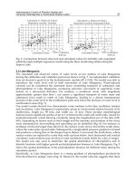
To illustrate the features of signal spectrums and filter frequency responses in coordinates of
complex frequency, the fig. 1 shows amplitude-frequency response schematics of IIR filter
and a spectral density module of input signal, if the following conditions apply: the filter
represents a series of low-pass second-order and first-order filters, and can be described by
complex amplitude vector
T
2,336
9,63 6,67
j
eG and complex frequency vector
T
= 150 640 400j q ; the input signal consists of an additive mixture of an unit step,
exponential component, semi-infinite sinusoidal component and damped oscillatory
component, and can be compactly described by complex amplitude vector
T
0,25
1 2 2
j j
e e
X
and complex frequency vector
T
0 120 300 40 500j j p .
Fig. 1. 3D amplitude signal spectrum and filter amplitude-frequency response
The 3D amplitude-frequency response (fig. 1) of the filter and signal spectrum module
shows, that complex frequencies of filter and input signal impulse functions have clearly
defined peaks.
This means, a 3D signal spectrum in complex frequency coordinates contains a continuous
spectrum along with four discrete lines on complex frequencies of input signal components.
The signal spectral densities on the mentioned complex frequencies are proportional to delta
Re( )
p
( )X p
( )K p
Im( )
p
The application of spectral representations in coordinates
of complex frequency for digital lter analysis and synthesis 33
2.
1
1
T
z e ,
0 1
( 1)/a z T
,
12
k T
;
3.
13 1
/(2 )k T T ,
13 1 1
(2 ) /(2 )z T T , complex frequency
13 13
ln( )/z T .
In cases of the first and third methods the coincidence of impulse function complex
frequencies of digital filter and analog filter-prototype is possible only if 0T . The second
method ensures the entire concurrence of complex frequencies of an analogue filter-
prototype and a digital filter in all instances. The later is very important, when the filter is
supposed to be used as a spectrum analyzer in coordinates of complex frequency.
The features of transition from a digital (discrete) filter, considering finite digit capacity
influence of microprocessor, including cases for filters with integer-valued coefficients, are
considered by the author in the research .
One of the most important advantages of the considered above approach to mathematical
description of FIR filters is obtaining FIR filter fast algorithms (Mokeev, 2008a, 2008b).
2.4 Overlapping the spectral and time approach
The impulse function (3) corresponds to the following differential equation
+ ( )
d t
t x t x t
dt
y
Ay B D C T ,
(7)
where
diagA q ,
B G
,
'
diagD G ;
T
( ) Re ( )
y
t tC y is a output signal of the filter.
In case of FIR filter (
D 0 ) the expression (7) is conform to one of known forms of state
space method. Thus, the application of mentioned spectral representations allows to
combine the spectral approach with the state space method for frequency filter analysis and
synthesis (Mokeev, 2008b, 2009b).
If one places the expression of generalized impulse characteristic (4) to the expression of
convolution integral, one will get the following expression of the filter output signal
( )
T
( )
t
t
t
y
t x e d
q
C T
G
.
(8)
If a generalized input signal (1) is fed into the filter input, simple input-output relations
(Mokeev, 2008b) can be gained on the base of the expression (8).
The expression (8) can be transformed into the following form
1
( )
m
M
t
m T m
m
y
t G X e ,
where ( , ) ( )
t
p
T
t T
X p t x e d
- is the instant spectrum of input signal in coordinates of
complex frequency.
Therefore, the elements of the vector
( )ty
are defined by solving M-number of independent
equations (7), each one of those can be interpreted as a value of instant (FIR filter) or current
(IIR filter) Laplace spectrum in corresponding complex frequency of filter impulse function
component.
The expression (7) is a generalization of one of state space method forms, and at the same
time directly connected with the Laplace spectral representations. So, one can view the
overlapping time approach (state space method) and frequency approach in complex
frequency coordinates.
On the base of analogue filter-prototype (7) descriptions, a mathematical expression of digital
filters can be obtained, by use of the known transition (synthesis) methods, applied to FIR
filters (Mokeev, 2008b). In this case fast algorithms for FIR filters are additionally synthesized.
2.5 Features of signal spectrum and filter frequency responses
in complex frequency coordinates
To illustrate the features of signal spectrums and filter frequency responses in coordinates of
complex frequency, the fig. 1 shows amplitude-frequency response schematics of IIR filter
and a spectral density module of input signal, if the following conditions apply: the filter
represents a series of low-pass second-order and first-order filters, and can be described by
complex amplitude vector
T
2,336
9,63 6,67
j
eG and complex frequency vector
T
= 150 640 400j q ; the input signal consists of an additive mixture of an unit step,
exponential component, semi-infinite sinusoidal component and damped oscillatory
component, and can be compactly described by complex amplitude vector
T
0,25
1 2 2
j j
e e
X
and complex frequency vector
T
0 120 300 40 500j j p .
Fig. 1. 3D amplitude signal spectrum and filter amplitude-frequency response
The 3D amplitude-frequency response (fig. 1) of the filter and signal spectrum module
shows, that complex frequencies of filter and input signal impulse functions have clearly
defined peaks.
This means, a 3D signal spectrum in complex frequency coordinates contains a continuous
spectrum along with four discrete lines on complex frequencies of input signal components.
The signal spectral densities on the mentioned complex frequencies are proportional to delta
Re( )
p
( )X p
( )K p
Im( )
p
Digital Filters34
function. Values of the transfer function on the mentioned complex frequencies of input
signal define a variation law of forced filter output signal components concerning input
signal components (Mokeev, 2007, 2008b). The rest of spectral regions characterize the
transient process in the filter due to step-by-step change of the input signal at the time zero.
A filters amplitude-frequency response is also three-dimensional and is represented by a
continuous spectrum and two discrete lines on complex frequencies of impulse function
components. In this case the values of the input signal representation of the above
mentioned complex frequencies, define a variation law of free components in relation to
filter impulse function components (Mokeev, 2007).
3. Filter analysis
3.1 Analysis methods based on features of signal and filter
spectral representations in complex frequency coordinates
Three methods of frequency filter analysis are suggested from the time-and-frequency
representations positions of signals and linear systems in coordinates of complex frequency
(Mokeev, 2007, 2008b).
The first method is based on the above considered features of signal spectrums and filter
frequency responses in complex frequency coordinates, and it allows for the determination
of forces and free filter components, by the use of simple arithmetic operations.
The other two methods are based on applied time-and-frequency representations of signals
or filters in coordinates of complex frequency. In this case instead of determining forced and
free components of the output filter signal, it is enough to consider the filter dynamic
properties by using only one of the mentioned component groups.
Based on time-and-frequency representations of signals and linear systems in coordinates of
complex frequency, the known definition by Charkevich A.A. (Kharkevich, 1960) for
accounting the dynamic properties of linear system is generalized:
1.
the signal is considered as current or instantaneous spectrum, and the system (filter) –
only as discrete components of frequency responses in coordinates of complex
frequency;
2.
the signal is characterized only by discrete components of spectrum, and the system
(filter) – by time dependence frequency responses.
Analysis methods for analog and digital IIR filters in case of semi-infinite input signals,
similar to (1), are considered below. These methods of filter analysis can be simply applied
to more complicated cases, for instance, to FIR filter (4) analysis at finite input signals
(Mokeev, 2008b).
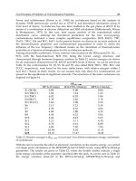
3.2 The first method of filter analysis: complex amplitude method generalization
The first method is a complex amplitude method generalization for definition of forced and
free components for filter reaction at semi-infinite or finite input signals.
The advantages of this method are related to simple algebraic operations, which are used for
determining the parameters of linear system reaction (filter, linear circuit) components to
input action described by a set of semi-infinite or finite damped oscillatory components.
Here, the expressions for determining forced and free components of analog and digital IIR
filter reaction to a signal, fed to filter input as a set of continuous or discrete damped
oscillatory components, i.e. for the generalized signal (1) and (2) at
'
X 0 , are given as
examples on fig. 2 and 3.
Fig. 2. Determining the forced components of an IIR filter output signal
Fig. 3. Determining the free components of an IIR filter output signal
The following notations are used in the expressions on fig. 2 and fig. 3:
( )X p or ( )X z , that
are the representations of the input signal without regard for phase shift of signal
components
T
e
q
Z .
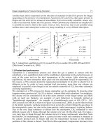
The example for determining the reaction (curve 1) of analog and digital (discrete) third-
order filter (condition in item 3.1), and the total forced (curve 2) and free (curve 3)
components is shown on the fig. 4. Using Matlab and Mathcad for determining the forced
and free components of an output signal, only complex amplitude vectors of an input signal
and filter impulse function , as well as the complex frequency vectors of an input signal and
filter are needed to be specified. The remaining calculations are carried out automatically.
0 0.01 0.02 0.03 0.04 0.05
0.05
0
0.05
Fig. 4. Determining the forced and free components of an output signal
The input-output expressions presented on fig. 2 and fig. 3 can be applied also to FIR filters
and finite signals (Mokeev, 2008b).
3.3 The second method: filter as a spectrum analyzer
The second method is based on interpreting a filter as an analyzer of current or instantaneous
spectrum of an input signal in coordinates of complex frequency (Mokeev, 2007, 2008b).
( )X z
T
2
( ) , ( ) Re ( , )
X y k Z kV Q G V Q
T
2
( ) , ( ) Re
t
X y t e
Q C t
V q G V
( )X p
T
, ( ) Re
t
g
t e
q
G G
T
, ( ) Re ( , )
g
k Z kG G Q
( )K z
T
, ( ) Re
t
t e
p
X x X
T
1
( ) , ( ) Re ,
K
y k Z kY Z X Y P
T
, ( ) Re ,
k Z kX x X P
T
1
( ) , ( ) Re
t
K
y t e
p
Y P X Y
( )K p
( ), ( )y t y k
, t kT
1
2
3
The application of spectral representations in coordinates
of complex frequency for digital lter analysis and synthesis 35
function. Values of the transfer function on the mentioned complex frequencies of input
signal define a variation law of forced filter output signal components concerning input
signal components (Mokeev, 2007, 2008b). The rest of spectral regions characterize the
transient process in the filter due to step-by-step change of the input signal at the time zero.
A filters amplitude-frequency response is also three-dimensional and is represented by a
continuous spectrum and two discrete lines on complex frequencies of impulse function
components. In this case the values of the input signal representation of the above
mentioned complex frequencies, define a variation law of free components in relation to
filter impulse function components (Mokeev, 2007).
3. Filter analysis
3.1 Analysis methods based on features of signal and filter
spectral representations in complex frequency coordinates
Three methods of frequency filter analysis are suggested from the time-and-frequency
representations positions of signals and linear systems in coordinates of complex frequency
(Mokeev, 2007, 2008b).
The first method is based on the above considered features of signal spectrums and filter
frequency responses in complex frequency coordinates, and it allows for the determination
of forces and free filter components, by the use of simple arithmetic operations.
The other two methods are based on applied time-and-frequency representations of signals
or filters in coordinates of complex frequency. In this case instead of determining forced and
free components of the output filter signal, it is enough to consider the filter dynamic
properties by using only one of the mentioned component groups.
Based on time-and-frequency representations of signals and linear systems in coordinates of
complex frequency, the known definition by Charkevich A.A. (Kharkevich, 1960) for
accounting the dynamic properties of linear system is generalized:
1.
the signal is considered as current or instantaneous spectrum, and the system (filter) –
only as discrete components of frequency responses in coordinates of complex
frequency;
2.
the signal is characterized only by discrete components of spectrum, and the system
(filter) – by time dependence frequency responses.
Analysis methods for analog and digital IIR filters in case of semi-infinite input signals,
similar to (1), are considered below. These methods of filter analysis can be simply applied
to more complicated cases, for instance, to FIR filter (4) analysis at finite input signals
(Mokeev, 2008b).
3.2 The first method of filter analysis: complex amplitude method generalization
The first method is a complex amplitude method generalization for definition of forced and
free components for filter reaction at semi-infinite or finite input signals.
The advantages of this method are related to simple algebraic operations, which are used for
determining the parameters of linear system reaction (filter, linear circuit) components to
input action described by a set of semi-infinite or finite damped oscillatory components.
Here, the expressions for determining forced and free components of analog and digital IIR
filter reaction to a signal, fed to filter input as a set of continuous or discrete damped
oscillatory components, i.e. for the generalized signal (1) and (2) at
'
X 0 , are given as
examples on fig. 2 and 3.
Fig. 2. Determining the forced components of an IIR filter output signal
Fig. 3. Determining the free components of an IIR filter output signal
The following notations are used in the expressions on fig. 2 and fig. 3:
( )X p or ( )X z , that
are the representations of the input signal without regard for phase shift of signal
components
T
e
q
Z .
The example for determining the reaction (curve 1) of analog and digital (discrete) third-
order filter (condition in item 3.1), and the total forced (curve 2) and free (curve 3)
components is shown on the fig. 4. Using Matlab and Mathcad for determining the forced
and free components of an output signal, only complex amplitude vectors of an input signal
and filter impulse function , as well as the complex frequency vectors of an input signal and
filter are needed to be specified. The remaining calculations are carried out automatically.
0 0.01 0.02 0.03 0.04 0.05
0.05
0
0.05
Fig. 4. Determining the forced and free components of an output signal
The input-output expressions presented on fig. 2 and fig. 3 can be applied also to FIR filters
and finite signals (Mokeev, 2008b).
3.3 The second method: filter as a spectrum analyzer
The second method is based on interpreting a filter as an analyzer of current or instantaneous
spectrum of an input signal in coordinates of complex frequency (Mokeev, 2007, 2008b).
( )X z
T
2
( ) , ( ) Re ( , )
X y k Z kV Q G V Q
T
2
( ) , ( ) Re
t
X y t e
Q C t
V q G V
( )X p
T
, ( ) Re
t
g
t e
q
G G
T
, ( ) Re ( , )
g
k Z kG G Q
( )K z
T
, ( ) Re
t
t e
p
X x X
T
1
( ) , ( ) Re ,
K
y k Z kY Z X Y P
T
, ( ) Re ,
k Z kX x X P
T
1
( ) , ( ) Re
t
K
y t e
p
Y P X Y
( )K p
( ), ( )y t y k
, t kT
1
2
3
Digital Filters36
If one converts the expression for an IIR filter complex impulse function (4) into an
expression of convolution integral, the result will be the dependence for a filter output
signal:
T
0
( ) ( ) ( ) ( , )
t
t
y
t x
g
t d X t e
q
G Q ,
(9)
where
0
( , ) ( )
t
p
X
p
t x e d
- is the current spectral density of an input signal, using Laplace
transform.
On the base of the expression (9) the calculations for determining a filter output signal
components are gained and represented on the fig. 5.
Fig. 5. Determining the IIR filter reaction
As concluded from the expression above, an IIR filter output signal depends on values of
the current Laplace spectrum of an input signal on filter impulse function complex
frequencies. Thus, a FIR filter is an analyzer of a signal instantaneous spectrum in a
coordinates of complex frequency.
3.4 The third method: diffusion of time-and-frequency approach to transfer function
The time-and-frequency approach in the third analysis method applies to a filter transfer
function, i.e. time dependent transfer function of the filter is used.
If one places the expression for a complex semi-infinite input signal (1) into the expression
for convolution integral, one will obtain the following dependence
T
0
( ) ( ) ( ) ( , )
t
t
y
t x
g
t d K t e
p
X P ,
where
0
( , ) ( )
t
p
K
p
t
g
e d - is time dependent transfer function of filter.
Then the input-output dependence for an IIR filter (4), when it is fed to semi-infinite input
signal, can be compactly presented in the following way (fig. 6).
Fig. 6. Filter reaction determination
Thus, a function modulus
( , )
n
K p t value on the complex frequency of n-th input signal
component describes the variation law of n-th component envelope of filter output signal.
X
( ) ( , )t K tY P X
T
( ) Re
t
x
t e
p
X
T
( ) Re ( )
t
y
t t e
p
Y
( , )
K
p t
G
( ) ( , )t X tV Q G
T
( ) Re
t
g
t e
q
G
T
( ) Re ( )
t
y
t t e
q
V
( , )X p t
The function argument characterizes phase change of the later mentioned output signal
component. Since the transient processes in filter are completed, the complex amplitude
( )
n
Y t will coincide with the complex amplitude of the forced component
n
Y .
In that case, filter amplitude-frequency and phase-frequency functions will be a three-
variable functions, i.e. it is necessary to represent responses in 4D space. For practical
visualization of frequency responses the approach, based on use of three-dimensional
frequency responses at complex frequency real or imaginary partly fixed value, can be
applied.
Let us consider the example from the item 3.1. The plot, shown on fig. 7 , is proportional to
the product
4
4
( , )
t
K j t e
. This plot on the complex frequency
4 4 4
p
j
is equal
to the envelope (curve 1 and 2) of filter reaction (curve 3) on the fourth component’s input
action for the filter input signal.
Fig. 7. Plot of the function
4
4
( , )
t
K j t e
The advantages of these suggested analysis methods, comparing to the existing ones for
specified generalized models of input signals and frequency filters, consist in calculation
simplicity, including solving problems of determining the performance parameters of signal
processing by frequency filters.
4. Filter synthesis
4.1 IIR filter synthesis
The application of spectral representations in complex frequency coordinates allows to
simplify significantly solving problems of filter synthesis for generalized signal model (1).
4
4
( , )
t
K j t e
3
t
1
2
The application of spectral representations in coordinates
of complex frequency for digital lter analysis and synthesis 37
If one converts the expression for an IIR filter complex impulse function (4) into an
expression of convolution integral, the result will be the dependence for a filter output
signal:
T
0
( ) ( ) ( ) ( , )
t
t
y
t x
g
t d X t e
q
G Q ,
(9)
where
0
( , ) ( )
t
p
X
p
t x e d
- is the current spectral density of an input signal, using Laplace
transform.
On the base of the expression (9) the calculations for determining a filter output signal
components are gained and represented on the fig. 5.
Fig. 5. Determining the IIR filter reaction
As concluded from the expression above, an IIR filter output signal depends on values of
the current Laplace spectrum of an input signal on filter impulse function complex
frequencies. Thus, a FIR filter is an analyzer of a signal instantaneous spectrum in a
coordinates of complex frequency.
3.4 The third method: diffusion of time-and-frequency approach to transfer function
The time-and-frequency approach in the third analysis method applies to a filter transfer
function, i.e. time dependent transfer function of the filter is used.
If one places the expression for a complex semi-infinite input signal (1) into the expression
for convolution integral, one will obtain the following dependence
T
0
( ) ( ) ( ) ( , )
t
t
y
t x
g
t d K t e
p
X P ,
where
0
( , ) ( )
t
p
K
p
t
g
e d - is time dependent transfer function of filter.
Then the input-output dependence for an IIR filter (4), when it is fed to semi-infinite input
signal, can be compactly presented in the following way (fig. 6).
Fig. 6. Filter reaction determination
Thus, a function modulus
( , )
n
K p t value on the complex frequency of n-th input signal
component describes the variation law of n-th component envelope of filter output signal.
X
( ) ( , )t K tY P X
T
( ) Re
t
x
t e
p
X
T
( ) Re ( )
t
y
t t e
p
Y
( , )
K
p t
G
( ) ( , )t X tV Q G
T
( ) Re
t
g
t e
q
G
T
( ) Re ( )
t
y
t t e
q
V
( , )X p t
The function argument characterizes phase change of the later mentioned output signal
component. Since the transient processes in filter are completed, the complex amplitude
( )
n
Y t will coincide with the complex amplitude of the forced component
n
Y .
In that case, filter amplitude-frequency and phase-frequency functions will be a three-
variable functions, i.e. it is necessary to represent responses in 4D space. For practical
visualization of frequency responses the approach, based on use of three-dimensional
frequency responses at complex frequency real or imaginary partly fixed value, can be
applied.
Let us consider the example from the item 3.1. The plot, shown on fig. 7 , is proportional to
the product
4
4
( , )
t
K j t e
. This plot on the complex frequency
4 4 4
p
j is equal
to the envelope (curve 1 and 2) of filter reaction (curve 3) on the fourth component’s input
action for the filter input signal.
Fig. 7. Plot of the function
4
4
( , )
t
K j t e
The advantages of these suggested analysis methods, comparing to the existing ones for
specified generalized models of input signals and frequency filters, consist in calculation
simplicity, including solving problems of determining the performance parameters of signal
processing by frequency filters.
4. Filter synthesis
4.1 IIR filter synthesis
The application of spectral representations in complex frequency coordinates allows to
simplify significantly solving problems of filter synthesis for generalized signal model (1).
4
4
( , )
t
K j t e
3
t
1
2
Digital Filters38
Let us consider robust filter synthesis, which have low sensitivity to change of useful signal
and disturbance parameters (Sánchez Peña, 1998). In other words, robust filters must ensure
the required signal performance factors at any possible variation of useful signal and
disturbance parameters, influencing on their spectrums. If one takes into account only two
main performance factors of signals: speed and accuracy, it will be enough to assure
fulfillment of requirements, connected to limitations for filter transfer function module on
complex frequency of useful signal and disturbance components (Mokeev, 2009c).
Thus, filter synthesis problem, instead of setting the requirements to particular frequency
response domains (pass band and rejection band), comes to form the dependences for filter
transfer function on complex frequencies of input signal components. To ensure the
required performance signal factors, it is necessary to consider possible variation ranges of
mentioned complex frequencies.
The synthesis will be carried out with increasing numbers of impulse function components
(4) till the achievement of the specified performance signal factors.
The block diagram, shown on fig. 8, illustrates the synthesis of optimal analogue filter-
prototype.
Fig. 8. Block diagram of optimal filter
The useful signal
0
( )x t
and the disturbance
( )
n
x t
on the graph _ are completely determined
by complex amplitude vectors
0
X
,
n
X
and complex frequency vectors
0
p ,
n
p . The vectors
of complex amplitudes and input signal frequencies are characterized as
T
0
n
X X X
,
T
0
n
p p p . In case of the value of the transformation operator ( ) 1H p , the error vector-
function is
0
( ) ( ) ( )t y t x t , in the rest of cases : ( ) ( ) ( )t y t z t .
Limitations on forced component level for IIR filter are set by the limitations on filter amplitude-
frequency response in complex frequency coordinates. Therefore, the problem of fulfillment of
signal processing accuracy requirements in filter operation stationary mode is completely solved,
and the filter speed
will be determined by transient process duration in the filter, i.e. by free
component damping below the permissible level (less than acceptable error of signal processing).
Free components damping can be approximately determined by the sum of their envelopes.
Thus, filter synthesis at specified structure comes to determination of its parameters, at
which the specified requirements to frequency responses in complex frequency coordinates
are ensured, and to ascertain the minimum time for signal processing performance
requirements guaranteeing. One more suggested method, that enables to simplify optimal
filter estimation, is related to use of time dependent filter transfer function
,K
p
t .
( )K p
( )H p
( )y t
( )
z
t
( )t
0
T
0 0
( ) Re
t
x
t e
p
X
T
( ) Re
n
t
n n
x
t e
p
X
T
( ) Re
t
x
t e
p
X
For searching the optimal solution it is reasonable to apply the realization in Optimization
Toolbox package, a part of MATLAB system of nonlinear optimization procedure methods
with the limitations to a filter transfer function value on specified complex frequencies of
input signal components and filter speed.
Order of filter synthesis, according to specified block diagram (fig. 8), consists in the
following. Type and filter order are given on the basis of features of solving problem, target
function and restrictions on filter frequency response values in complex frequency
coordinates are formed based on ensuring of signal processing performance required
parameters. Then filter parameters are calculated with use of optimization procedures. In
case of the found solution does not meet signal processing performance requirements, the
order of filter should be raised and filter parameters should be found again.
Let us consider an example of analogue filter-prototype synthesis to separate the sine signal
against a disturbance background in the exponential component form.
To extract the useful signal and eliminate the disturbance, acceptable speed can be only be
obtained with use of second-order and higher order filters. Let us consider second-order
high-pass filter synthesis.
The main phases of IIR filter synthesis for selection industrial frequency useful signal
against a background of exponential disturbance are presented in table 4.
№ Name Conditions
1.
Input signal
2
1 1 2
( ) cos
t
m
x t X t X e
limits of useful signal frequency variation
1
2 45 55 rad/s,
maximum disturbance level
2 1m
X X ,
changing size of damping coefficient
1
2
0 200 s
2.
Signal processing
performance requirements
1.
acceptable error in signal processing:
automation function
1
0,1 (5 %),
metering function
2
0,01 (1 %),
2.
speed:
1
20
мс (5%),
2
40
ms (1%),
3.
acceptable overshoot level:
10%
3.
Requirements to filter
amplitude-frequency
response in complex
frequency coordinates
1.
section
p j
:
0
1K j
,
0
100 rad/s,
2 0 2
1 1K j ,
10 rad/s
2.
section
p
:
1
1
( )K e ,
2
2
( )K e
4.
Transfer function of second-
order high-pass filter
2
2 2
0,874
224 221
p
K p
p p
Table 4. IIR filter synthesis
The amplitude-frequency responses in the sections
p
j
and
p
(at
1
0,02 s
) are
represented on fig. 9. On fig. 9 along with filter amplitude-frequency response the
limitations on filter amplitude-frequency response values, according to the requirements in
table 4 item 3, are shown. Amplitude-frequency response value out of mentioned
restrictions zone conventionally is
1
. As follows from the fig. 9, the synthesized filter
completely meets the requirements of signal processing accuracy at frequency change 5
Hz in power system.
The application of spectral representations in coordinates
of complex frequency for digital lter analysis and synthesis 39
Let us consider robust filter synthesis, which have low sensitivity to change of useful signal
and disturbance parameters (Sánchez Peña, 1998). In other words, robust filters must ensure
the required signal performance factors at any possible variation of useful signal and
disturbance parameters, influencing on their spectrums. If one takes into account only two
main performance factors of signals: speed and accuracy, it will be enough to assure
fulfillment of requirements, connected to limitations for filter transfer function module on
complex frequency of useful signal and disturbance components (Mokeev, 2009c).
Thus, filter synthesis problem, instead of setting the requirements to particular frequency
response domains (pass band and rejection band), comes to form the dependences for filter
transfer function on complex frequencies of input signal components. To ensure the
required performance signal factors, it is necessary to consider possible variation ranges of
mentioned complex frequencies.
The synthesis will be carried out with increasing numbers of impulse function components
(4) till the achievement of the specified performance signal factors.
The block diagram, shown on fig. 8, illustrates the synthesis of optimal analogue filter-
prototype.
Fig. 8. Block diagram of optimal filter
The useful signal
0
( )x t
and the disturbance
( )
n
x t
on the graph _ are completely determined
by complex amplitude vectors
0
X
,
n
X
and complex frequency vectors
0
p ,
n
p . The vectors
of complex amplitudes and input signal frequencies are characterized as
T
0
n
X X X
,
T
0
n
p p p . In case of the value of the transformation operator
( ) 1H p , the error vector-
function is
0
( ) ( ) ( )t y t x t , in the rest of cases :
( ) ( ) ( )t y t z t .
Limitations on forced component level for IIR filter are set by the limitations on filter amplitude-
frequency response in complex frequency coordinates. Therefore, the problem of fulfillment of
signal processing accuracy requirements in filter operation stationary mode is completely solved,
and the filter speed
will be determined by transient process duration in the filter, i.e. by free
component damping below the permissible level (less than acceptable error of signal processing).
Free components damping can be approximately determined by the sum of their envelopes.
Thus, filter synthesis at specified structure comes to determination of its parameters, at
which the specified requirements to frequency responses in complex frequency coordinates
are ensured, and to ascertain the minimum time for signal processing performance
requirements guaranteeing. One more suggested method, that enables to simplify optimal
filter estimation, is related to use of time dependent filter transfer function
,K
p
t .
( )K p
( )H p
( )y t
( )
z
t
( )t
0
T
0 0
( ) Re
t
x
t e
p
X
T
( ) Re
n
t
n n
x
t e
p
X
T
( ) Re
t
x
t e
p
X
For searching the optimal solution it is reasonable to apply the realization in Optimization
Toolbox package, a part of MATLAB system of nonlinear optimization procedure methods
with the limitations to a filter transfer function value on specified complex frequencies of
input signal components and filter speed.
Order of filter synthesis, according to specified block diagram (fig. 8), consists in the
following. Type and filter order are given on the basis of features of solving problem, target
function and restrictions on filter frequency response values in complex frequency
coordinates are formed based on ensuring of signal processing performance required
parameters. Then filter parameters are calculated with use of optimization procedures. In
case of the found solution does not meet signal processing performance requirements, the
order of filter should be raised and filter parameters should be found again.
Let us consider an example of analogue filter-prototype synthesis to separate the sine signal
against a disturbance background in the exponential component form.
To extract the useful signal and eliminate the disturbance, acceptable speed can be only be
obtained with use of second-order and higher order filters. Let us consider second-order
high-pass filter synthesis.
The main phases of IIR filter synthesis for selection industrial frequency useful signal
against a background of exponential disturbance are presented in table 4.
№ Name Conditions
1.
Input signal
2
1 1 2
( ) cos
t
m
x t X t X e
limits of useful signal frequency variation
1
2 45 55 rad/s,
maximum disturbance level
2 1m
X X ,
changing size of damping coefficient
1
2
0 200 s
2.
Signal processing
performance requirements
1. acceptable error in signal processing:
automation function
1
0,1 (5 %),
metering function
2
0,01 (1 %),
2. speed:
1
20
мс (5%),
2
40
ms (1%),
3. acceptable overshoot level:
10%
3.
Requirements to filter
amplitude-frequency
response in complex
frequency coordinates
1.
section
p j
:
0
1K j
,
0
100 rad/s,
2 0 2
1 1K j , 10 rad/s
2. section
p
:
1
1
( )K e ,
2
2
( )K e
4.
Transfer function of second-
order high-pass filter
2
2 2
0,874
224 221
p
K p
p p
Table 4. IIR filter synthesis
The amplitude-frequency responses in the sections
p
j
and
p
(at
1
0,02 s
) are
represented on fig. 9. On fig. 9 along with filter amplitude-frequency response the
limitations on filter amplitude-frequency response values, according to the requirements in
table 4 item 3, are shown. Amplitude-frequency response value out of mentioned
restrictions zone conventionally is
1 . As follows from the fig. 9, the synthesized filter
completely meets the requirements of signal processing accuracy at frequency change 5
Hz in power system.
Digital Filters40
The plot of transient process in second-order high-pass filter at signal feeding (table 4 point
1) is presented on fig. 10. The transient process durations are 11 ms (that is 10% of
acceptable error), 15 ms (5%) and 33 ms (1%) at any exponential component damping
coefficient value from the specified range
0 200
s
-1
.
Fig. 9. Filter amplitude-frequency response in the sections
2
p
j f
and
p
0 0.01 0.02 0.03 0.04 0.05
1
0
1
Fig. 10. Filter output signal
Therefore, synthesized second-order high-pass filter has low sensitivity to exponential
component damping coefficient variation and to power system frequency deviation.
This example clearly illustrates the advantages of using the Laplace transform spectral
representations for frequency filter synthesis. Applying these representations in
combination with multidimensional optimization methods with the contingencies enables to
perform frequency filter synthesis for problems, that were unsolvable at traditional spectral
representations usage (Mokeev, 2008b). For instance, for the problem of filter synthesis for
separation of the following signals: constant and exponential signals, two exponential
signals with non-overlapping damping coefficient change ranges, sinusoidal and damped
oscillatory components with equal or similar frequencies.
The mentioned above synthesis method can be also effectively apply for typical signal
filtering problems, including problems of useful signal extraction against the white noise. In
1
2
f
0 50 100 150 200
0
0.5
1
( )K
j
1
2
45 50 55
0
.98
1
0 100 200 300
0
0.05
1
2
0.02
( )K e
( )y t
t
that, the white noise realizations can be described by the special case of generalized signal
model (1) as a set of time-shifted fast damping exponents of different digits. Initial values
and appearance time of the mentioned exponential components are random variables,
which variation law ensures the white noise specified spectral characteristics. This white
noise model allows to approach filter synthesis on the basis of the signal spectral
representation features (1) in complex frequency coordinates and to guarantee the required
combinations of signal processing speed and accuracy (Mokeev, 2008b).
4.2 FIR filter synthesis
Comparing to IIR filter synthesis, synthesis of FIR filters is significantly simpler due to
easier control over transient processes duration in filter. In case of compliance with the
restrictions on amplitude-frequency response values on input signal complex frequencies
(1), filter speed will be determined by the length of its impulse response.
As examples of synthesis, let us consider averaging FIR filter synthesis for intellectual
electronic devices (IED) of electric power systems. Block diagram of the most widespread
signal processing algorithm is given on Fig. 11.
Fig. 11. Block diagram for signal processing
There is the input-output dependence for the considered algorithm
0
1
( )
t t
j
t T t T
X t e w t d x w t d
.
This expression corresponds to short-time Fourier transform on the frequency
0
.
Frequency filtering efficiency depends much to a large extent on the choice (synthesis) of
time window
w t , or on filter impulse function, that is equivalent for averaging filter.
Let us consider input signal as a set of complex amplitudes and exponential disturbance
frequencies, industrial frequency useful signal
1
and higher harmonics
T
0 1 2 3 N
X X X X X
X
,
T
0 1 1 1 1
2 3 4j j j j p
.
(10)
If one separates the exponential component and denotes the vector for harmonic complex
amplitudes by
1
X
, the filter input signal can be presented in the following way
1 0 1 0
0
( )
T T
0 1 1
( ) 2 2 2
j
t
j
t
j t
x t X e e e
n n
X X
,
where the vector
1
X consists of conjugate to the vector
1
X elements.
When nominal frequency of power system is
1 0
,
0 0
0 0
1 1
( ) 2
0 1 1
2
( ) 2
N
j
n t j n t
j t j t
n n
n
x t X e X X e X e X e
.
( )K p
T
( ) Re
t
t e
p
X
1
( ) ( )
y
t X t
0
2
j
t
e
0 0
T T
( ) 2 2
j
t
j
t
x t e e
p p
X X
The application of spectral representations in coordinates
of complex frequency for digital lter analysis and synthesis 41
The plot of transient process in second-order high-pass filter at signal feeding (table 4 point
1) is presented on fig. 10. The transient process durations are 11 ms (that is 10% of
acceptable error), 15 ms (5%) and 33 ms (1%) at any exponential component damping
coefficient value from the specified range
0 200
s
-1
.
Fig. 9. Filter amplitude-frequency response in the sections
2
p
j f
and
p
0 0.01 0.02 0.03 0.04 0.05
1
0
1
Fig. 10. Filter output signal
Therefore, synthesized second-order high-pass filter has low sensitivity to exponential
component damping coefficient variation and to power system frequency deviation.
This example clearly illustrates the advantages of using the Laplace transform spectral
representations for frequency filter synthesis. Applying these representations in
combination with multidimensional optimization methods with the contingencies enables to
perform frequency filter synthesis for problems, that were unsolvable at traditional spectral
representations usage (Mokeev, 2008b). For instance, for the problem of filter synthesis for
separation of the following signals: constant and exponential signals, two exponential
signals with non-overlapping damping coefficient change ranges, sinusoidal and damped
oscillatory components with equal or similar frequencies.
The mentioned above synthesis method can be also effectively apply for typical signal
filtering problems, including problems of useful signal extraction against the white noise. In
1
2
f
0 50 100 150 200
0
0.5
1
( )K
j
1
2
45 50 55
0
.98
1
0 100 200 300
0
0.05
1
2
0.02
( )K e
( )y t
t
that, the white noise realizations can be described by the special case of generalized signal
model (1) as a set of time-shifted fast damping exponents of different digits. Initial values
and appearance time of the mentioned exponential components are random variables,
which variation law ensures the white noise specified spectral characteristics. This white
noise model allows to approach filter synthesis on the basis of the signal spectral
representation features (1) in complex frequency coordinates and to guarantee the required
combinations of signal processing speed and accuracy (Mokeev, 2008b).
4.2 FIR filter synthesis
Comparing to IIR filter synthesis, synthesis of FIR filters is significantly simpler due to
easier control over transient processes duration in filter. In case of compliance with the
restrictions on amplitude-frequency response values on input signal complex frequencies
(1), filter speed will be determined by the length of its impulse response.
As examples of synthesis, let us consider averaging FIR filter synthesis for intellectual
electronic devices (IED) of electric power systems. Block diagram of the most widespread
signal processing algorithm is given on Fig. 11.
Fig. 11. Block diagram for signal processing
There is the input-output dependence for the considered algorithm
0
1
( )
t t
j
t T t T
X t e w t d x w t d
.
This expression corresponds to short-time Fourier transform on the frequency
0
.
Frequency filtering efficiency depends much to a large extent on the choice (synthesis) of
time window
w t , or on filter impulse function, that is equivalent for averaging filter.
Let us consider input signal as a set of complex amplitudes and exponential disturbance
frequencies, industrial frequency useful signal
1
and higher harmonics
T
0 1 2 3 N
X X X X X
X
,
T
0 1 1 1 1
2 3 4j j j j p
.
(10)
If one separates the exponential component and denotes the vector for harmonic complex
amplitudes by
1
X
, the filter input signal can be presented in the following way
1 0 1 0
0
( )
T T
0 1 1
( ) 2 2 2
j
t
j
t
j t
x t X e e e
n n
X X
,
where the vector
1
X consists of conjugate to the vector
1
X elements.
When nominal frequency of power system is
1 0
,
0 0
0 0
1 1
( ) 2
0 1 1
2
( ) 2
N
j
n t j n t
j t j t
n n
n
x t X e X X e X e X e
.
( )K p
T
( ) Re
t
t e
p
X
1
( ) ( )
y
t X t
0
2
j
t
e
0 0
T T
( ) 2 2
j
t
j
t
x t e e
p p
X X
Digital Filters42
Thus, averaging FIR filter at
1 0
must ensure the separation of constant component
1
X
and elimination of damped oscillatory component, sinusoidal component with double to
industrial frequency, related to useful signal transform , and also of higher harmonics with
frequencies multiple of
0
. In case of
1 0
, useful input signal of averaging filter will be
a low-frequency sine signal with the frequency
1 0
.
In filter synthesis the following signal parameters should be taken into account: the
exponential disturbance damping coefficient changes in signal
( )x t
, power system
frequency and related to it useful signal and disturbance changes, which influence on signal
spectral composition and useful signal-disturbance ratio.
Let us consider averaging FIR filters synthesis for PMU (Phasor Measurement Units) devices
and compare the gained results with averaging FIR filters, applied in one of the best PMU –
Model 1133A Power Sentinel, made by American company Arbiter (Gustafson, 2009).
In this PMU one of the following time windows can be implemented: Raised cosine, Hann,
Hamming, Blackman, Bartlett, Rectangular, Flat Top, Kaiser, Nutall 4-term, at any filter
length, which can be from one to several periods of industrial frequency
0 0
2 /T
.
First let us find the solutions without consideration of exponential disturbance elimination,
as it is accepted in the most of PMU (Phadke, 2008). The filter must guarantee less than 40
ms speed and 0.2 accuracy class.
Let us accept the following parameters for FIR filter generalized impulse function:
T
'
0 1 2 3 4
G G G G G G G
,
T
1 1 1 1
0 2 3 4jw j w j w j wq
,
T
1 1 1 1 1
T T T T TT
,
1 1
2 /T w
.
This special case corresponds to so-called generalized cosine time window (Smith, 2002).
This type of window will be further described by the set of only two parameters:
G
and
1
T .
Optimization procedure and target function choice of is a nontrivial problem. In general, in
case of several synthesis purposes (criteria), it is complicated to get a rigorous optimal
solution. Therefore, the found solutions for averaging FIR filters, should be considered as
suboptimal.
Let us consider averaging FIR filters synthesis with use of nonlinear multivariable method,
based on function of The Optimization Toolbox extends of MATLAB system. The found
solutions at different filter lengths are given in table 5 and on fig. 12.
№
G
1
T
, с
1.
T
98,8842 0,2601 0, 4843 0,2325 0,0231 0
0,0401
2.
T
101,0814 0,2827 0,5148 0,1983 0,0058 0,0016
0,0350
3.
T
70,027 0,3989 0,4976 0,1015 0,0021 0,0001
0,0358
4.
T
73,505 0, 4535 0,4953 0,0547 0 0,0034
0,0300
5.
T
77,691 0,5108 0,4819 0,0204 0,0014 0,0145
0,0252
6.
T
82,7152 0,5397 0,4651 0,0072 0 0,0121
0,0224
Table 5. Averaging FIR filter parameters
Fig. 12. Amplitude-frequency responses of FIR filters
The impulse functions (time windows) of synthesized filters are presented on fig. 13.
Fig. 13. Time windows of averaging FIR filters
As follows from the fig. 12, filters 1 and 2 have significantly better metrological
performances, than averaging FIR filters PMU 1133A.
Filters 3÷6 are used in algorithms of IED signal processing, which do not need ensuring of
amplitude-frequency responses stability over the range 0÷5 Hz, according to specified
accuracy class (Mokeev, 2009c). Besides that, the more amplitude-frequency responses will be
reduced with the frequency growth and the more harmonic elimination with the frequency
about 100 Hz there will be, the more exactly the power system frequency will be determined
1 1
1 1
1 0
2
1
( ) ( )
( ) ( )
( )
c s
s c
m
dX t dX t
X t X t
dt dt
t
X t
,
(11)
where
1 1 1
( ) ( ) ( )
c s
X t X t
j
X t
.
Although the mentioned algorithms of signal processing are adaptive, stationary filters are
used in them. Signal processing error, connected to amplitude-frequency response deviation
from 1 over the range from 0 to 5 Hz, can be easily compensated due to frequency
measurement according to (11).
0 0.005 0.01 0.015 0.02 0.025 0.03 0.035 0.04
0
0.5
1
( )g t
1
2
3
4
5
6
t
0 50 100 150 200 250 300 350 400
0
0.5
1
2K j f
1
2
3
4
5
6
0 2 4
0.98
0.99
1
95 100 105
0
5
10
4
0.001
1 2
3
4
5
6
1
2
3
4
5
6
f
The application of spectral representations in coordinates
of complex frequency for digital lter analysis and synthesis 43
Thus, averaging FIR filter at
1 0
must ensure the separation of constant component
1
X
and elimination of damped oscillatory component, sinusoidal component with double to
industrial frequency, related to useful signal transform , and also of higher harmonics with
frequencies multiple of
0
. In case of
1 0
, useful input signal of averaging filter will be
a low-frequency sine signal with the frequency
1 0
.
In filter synthesis the following signal parameters should be taken into account: the
exponential disturbance damping coefficient changes in signal
( )x t
, power system
frequency and related to it useful signal and disturbance changes, which influence on signal
spectral composition and useful signal-disturbance ratio.
Let us consider averaging FIR filters synthesis for PMU (Phasor Measurement Units) devices
and compare the gained results with averaging FIR filters, applied in one of the best PMU –
Model 1133A Power Sentinel, made by American company Arbiter (Gustafson, 2009).
In this PMU one of the following time windows can be implemented: Raised cosine, Hann,
Hamming, Blackman, Bartlett, Rectangular, Flat Top, Kaiser, Nutall 4-term, at any filter
length, which can be from one to several periods of industrial frequency
0 0
2 /T
.
First let us find the solutions without consideration of exponential disturbance elimination,
as it is accepted in the most of PMU (Phadke, 2008). The filter must guarantee less than 40
ms speed and 0.2 accuracy class.
Let us accept the following parameters for FIR filter generalized impulse function:
T
'
0 1 2 3 4
G G G G G G G
,
T
1 1 1 1
0 2 3 4jw j w j w j wq
,
T
1 1 1 1 1
T T T T TT
,
1 1
2 /T w
.
This special case corresponds to so-called generalized cosine time window (Smith, 2002).
This type of window will be further described by the set of only two parameters:
G
and
1
T .
Optimization procedure and target function choice of is a nontrivial problem. In general, in
case of several synthesis purposes (criteria), it is complicated to get a rigorous optimal
solution. Therefore, the found solutions for averaging FIR filters, should be considered as
suboptimal.
Let us consider averaging FIR filters synthesis with use of nonlinear multivariable method,
based on function of The Optimization Toolbox extends of MATLAB system. The found
solutions at different filter lengths are given in table 5 and on fig. 12.
№
G
1
T
, с
1.
T
98,8842 0,2601 0, 4843 0,2325 0,0231 0
0,0401
2.
T
101,0814 0,2827 0,5148 0,1983 0,0058 0,0016
0,0350
3.
T
70,027 0,3989 0,4976 0,1015 0,0021 0,0001
0,0358
4.
T
73,505 0, 4535 0,4953 0,0547 0 0,0034
0,0300
5.
T
77,691 0,5108 0,4819 0,0204 0,0014 0,0145
0,0252
6.
T
82,7152 0,5397 0,4651 0,0072 0 0,0121
0,0224
Table 5. Averaging FIR filter parameters
Fig. 12. Amplitude-frequency responses of FIR filters
The impulse functions (time windows) of synthesized filters are presented on fig. 13.
Fig. 13. Time windows of averaging FIR filters
As follows from the fig. 12, filters 1 and 2 have significantly better metrological
performances, than averaging FIR filters PMU 1133A.
Filters 3÷6 are used in algorithms of IED signal processing, which do not need ensuring of
amplitude-frequency responses stability over the range 0÷5 Hz, according to specified
accuracy class (Mokeev, 2009c). Besides that, the more amplitude-frequency responses will be
reduced with the frequency growth and the more harmonic elimination with the frequency
about 100 Hz there will be, the more exactly the power system frequency will be determined
1 1
1 1
1 0
2
1
( ) ( )
( ) ( )
( )
c s
s c
m
dX t dX t
X t X t
dt dt
t
X t
,
(11)
where
1 1 1
( ) ( ) ( )
c s
X t X t
j
X t
.
Although the mentioned algorithms of signal processing are adaptive, stationary filters are
used in them. Signal processing error, connected to amplitude-frequency response deviation
from 1 over the range from 0 to 5 Hz, can be easily compensated due to frequency
measurement according to (11).
0 0.005 0.01 0.015 0.02 0.025 0.03 0.035 0.04
0
0.5
1
( )g t
1
2
3
4
5
6
t
0 50 100 150 200 250 300 350 400
0
0.5
1
2K j f
1
2
3
4
5
6
0 2 4
0.98
0.99
1
95 100 105
0
5
10
4
0.001
1 2
3
4
5
6
1
2
3
4
5
6
f
Digital Filters44
Let us do synthesis of averaging filter with use of FIR filter generalized model (4) at 2M ,
according to the requirements in table 6.
№ Name Conditions
1.
Changing sizes of filter
input signal parameters
(10)
1
2 45 55 rad/s,
1
0 2
,
0 1
0 1
m
X X ,
1
0
20 200 s ,
0 1
0 1
m
X X ,
1
0 0,5
n m
X X , 2n
2.
Signal processing
performance
requirements
1. Acceptable error:
1
0,001,
2
0,0015 (0,15 %),
additional error at power system frequency deviation:
2
0,0015 (0.15 %),
additional error at
0 1m
X X
,
1
0
20 200 s and
1
t T
:
3
0,03 (3 %),
2. speed:
1
0,06T s,
1
0,04 s
3. acce
p
table overshoot level:
10%
3.
Requirements to filter
amplitude-frequency
responses in complex
frequency coordinates
1.
section
p j
:
0 1K ,
12 12
1 1K j ,
0 1
2K j ,
0 12
2K j ,
0 12
2 0,5K j n
, 3n
where 10 rad/s,
12 1 2
2.
section
0
p j
:
1
0 3
2 ( )
T
K j e ,
1
0
2 ( ) 0.05K j e
Table 6. Averaging FIR filter synthesis
The lengths of all finite damped oscillatory components of filter impulse functions will be
considered as equal. Using different efficiency functions, two averaging FIR filters with
practically identical frequency responses were obtained:
T
4,232 0,5887
1
80,48 37,93
j j
e eG
,
T
1
22,99 62,30 23,26 186,9j jq ,
T
1 11 11
T TT
,
11
0,051T
с,
1 11
1
T 'T
1 1 1
( ) Re
t T
t
g t e e
q
q
G G
;
(12)
T
6,024 2,938
2
42,26 38,36
j j
e eG
,
T
2
4,668 42,69 23,28 178,7j jq ,
T
2 21 21
T TT
,
21
0,050T с,
2 21
2
T 'T
2 2 2
( ) Re
t T
t
g t e e
q
q
G G
.
(13)
Filter amplitude-frequency responses and their impulse responses (curve 1 and 2) are shown
on the fig. 14 and fig. 15. The averaging filters impulse responses as opposed to ones,
considered above (fig. 13), are asymmetrical. Therefore, the filters with mirror-inverse
impulse responses (curve 3 and 4) will have the same amplitude-frequency responses in the
sections
2
p
j f
, i.e.
3 1 11
( ) ( )g t g T t
and
4 2 21
( ) ( )g t g T t
. However, filter amplitude-
frequency responses with the numbers 3 and 4 in the section
0
p
j significantly differ
from the analogous amplitude-frequency responses of filters – ancestors (filters 1 and 2).
Thus, the principal conclusion follows from the above: the use of filter traditional
amplitude-frequency responses (the section 2
p
j f ) for aperiodic signals analysis is not
effective.
Fig. 14. Filter amplitude-frequency response in the section
2
p
j f
Fig. 15. Amplitude-frequency response in the section
0
p
j
and impulse responses
The principal difference filter 1 from filter 2 consists in the following: in the first case (filter
1) oscillatory nature of transient process will be observed in the beginning, in the second
case it will occur after transient process completes in the filter. As it follows from the fig. 16,
the combined use of filters 1 and 2 with practically identical amplitude-frequency response
enables to reveal the transient processes in filters (curve 3).
Fig. 16. Output signals of FIR filter
Synthesized filters ensure the combination of signal processing high speed and accuracy,
have a low sensitivity to power system frequency deviation and to disturbance spectrum
change, and significantly exceed filters, used in PMU 1133A.
0 50 100 150 200
0
0.5
1
2K j f
1
2
95 100 105
0
5
10
4
2
1
f
0 2 4
0.996
0.998
1
1.002
1.004
1
2
3
4
3
4
12
1
2
1
T
K e
( )g t
t
0 40 80 120 160 200
0
0.02
0.04
0 0.02 0.04
0
50
3
1
2
( )y t
t
0 0.01 0.02 0.03 0.04 0.05 0.06 0.07
0
0.5
1
The application of spectral representations in coordinates
of complex frequency for digital lter analysis and synthesis 45
Let us do synthesis of averaging filter with use of FIR filter generalized model (4) at 2M ,
according to the requirements in table 6.
№ Name Conditions
1.
Changing sizes of filter
input signal parameters
(10)
1
2 45 55 rad/s,
1
0 2
,
0 1
0 1
m
X X ,
1
0
20 200 s ,
0 1
0 1
m
X X ,
1
0 0,5
n m
X X , 2n
2.
Signal processing
performance
requirements
1.
Acceptable error:
1
0,001,
2
0,0015 (0,15 %),
additional error at power system frequency deviation:
2
0,0015 (0.15 %),
additional error at
0 1m
X X
,
1
0
20 200 s and
1
t T
:
3
0,03 (3 %),
2.
speed:
1
0,06T s,
1
0,04 s
3.
acce
p
table overshoot level:
10%
3.
Requirements to filter
amplitude-frequency
responses in complex
frequency coordinates
1.
section
p j
:
0 1K ,
12 12
1 1K j ,
0 1
2K j ,
0 12
2K j ,
0 12
2 0,5K j n
, 3n
where
10 rad/s,
12 1 2
2.
section
0
p j
:
1
0 3
2 ( )
T
K j e ,
1
0
2 ( ) 0.05K j e
Table 6. Averaging FIR filter synthesis
The lengths of all finite damped oscillatory components of filter impulse functions will be
considered as equal. Using different efficiency functions, two averaging FIR filters with
practically identical frequency responses were obtained:
T
4,232 0,5887
1
80,48 37,93
j j
e eG
,
T
1
22,99 62,30 23,26 186,9j jq ,
T
1 11 11
T TT
,
11
0,051T
с,
1 11
1
T 'T
1 1 1
( ) Re
t T
t
g t e e
q
q
G G
;
(12)
T
6,024 2,938
2
42,26 38,36
j j
e eG
,
T
2
4,668 42,69 23,28 178,7j jq ,
T
2 21 21
T TT
,
21
0,050T с,
2 21
2
T 'T
2 2 2
( ) Re
t T
t
g t e e
q
q
G G
.
(13)
Filter amplitude-frequency responses and their impulse responses (curve 1 and 2) are shown
on the fig. 14 and fig. 15. The averaging filters impulse responses as opposed to ones,
considered above (fig. 13), are asymmetrical. Therefore, the filters with mirror-inverse
impulse responses (curve 3 and 4) will have the same amplitude-frequency responses in the
sections
2
p
j f
, i.e.
3 1 11
( ) ( )g t g T t
and
4 2 21
( ) ( )g t g T t
. However, filter amplitude-
frequency responses with the numbers 3 and 4 in the section
0
p
j
significantly differ
from the analogous amplitude-frequency responses of filters – ancestors (filters 1 and 2).
Thus, the principal conclusion follows from the above: the use of filter traditional
amplitude-frequency responses (the section
2
p
j f ) for aperiodic signals analysis is not
effective.
Fig. 14. Filter amplitude-frequency response in the section
2
p
j f
Fig. 15. Amplitude-frequency response in the section
0
p
j and impulse responses
The principal difference filter 1 from filter 2 consists in the following: in the first case (filter
1) oscillatory nature of transient process will be observed in the beginning, in the second
case it will occur after transient process completes in the filter. As it follows from the fig. 16,
the combined use of filters 1 and 2 with practically identical amplitude-frequency response
enables to reveal the transient processes in filters (curve 3).
Fig. 16. Output signals of FIR filter
Synthesized filters ensure the combination of signal processing high speed and accuracy,
have a low sensitivity to power system frequency deviation and to disturbance spectrum
change, and significantly exceed filters, used in PMU 1133A.
0 50 100 150 200
0
0.5
1
2K j f
1
2
95 100 105
0
5
10
4
2
1
f
0 2 4
0.996
0.998
1
1.002
1.004
1
2
3
4
3
4
12
1
2
1
T
K e
( )g t
t
0 40 80 120 160 200
0
0.02
0.04
0 0.02 0.04
0
50
3
1
2
( )y t
t
0 0.01 0.02 0.03 0.04 0.05 0.06 0.07
0
0.5
1
Digital Filters46
The following regularities of time windows for averaging FIR filters can be defined on
example of filter synthesis for special case
1. in case of using the cosine time windows and/or time windows (4) at harmonic input
signals the form of the synthesized windows is similar to symmetrical “bell-shaped” or
in the form of “hat” (fig. 13);
2.
in case of using the general time windows (4) at necessity of aperiodic disturbance
elimination the windows with clearly defined asymmetrical form (fig. 15) are obtained.
Therefore, the fact can be stated, that for processing of compound semi-infinite or finite
aperiodic input signals it is reasonable to use the FIR filter impulse functions (4).
Considering the relation between filters and wavelet transforms Koronovskii, 2005, Lyons,
2004), the conclusion about reasonability of mother and father wavelets synthesis, based on
the expression (4), can be made. The transition from the mathematical description of
analogue filter-prototype to digital filter is carried out by one of the following known
methods with the consideration of analog FIR filter specifics (Mokeev, 2008b).
5. Fast algorithms synthesis of FIR filters and spectrum analyzers
5.1 FIR filter fast algorithms synthesis, based on generalized
model of analogue filter-prototype impulse function
The advantage of using the analogue filter-prototypes with finite impulse response is direct
synthesis of FIR filter realization fast (recursive) algorithms, according to the chosen
modified transition method under the table 3.
The fast (recursive) algorithm for general case, using the first or second synthesis methods,
is given below
( ) ( ) ( ) ( 1)k x k x k y k y A B C N D
,
T
( ) Re ( )
y
k k C y
.
(14)
where for the first method
1
1
m m
M
G T T
A
,
1
'
1
m m
M
G T T
B
,
1
1
m
M
T
D
,
1
M
C ,
m
M
NN ; for the second method
m
M
G T
A
,
'
m
M
G T
B
,
m
T
M
e
D
.
The block scheme of FIR filter (14) fast (recursive) algorithm is represented on the fig. 17,
where
m
N
M
z
Z
.
Fig. 17. FIR filter fast algorithm
( )
x
k
A
1
ky
D
ky
Z
( )
x
k
C N
B
IIR filter
+
( )y k
1
z
T
C
The fast algorithm (14) expression form, using matrixes, is a compact way of algorithm
expression, however, there is a system of M-number independent equations in case of
practical realization.
( ) ( ) ( ) ( 1)
m m m m m
y k a x k b x k N d y k
,
(15)
where
m
a ,
m
b ,
m
d - are complex coefficients, which are the m-th elements of A , B , D
vectors.
The fast algorithm (14) or (15) can be directly realized by using DSPs, which include the
instructions to multiplication with accumulation. At other cases, it is necessary to divide the
algorithm (15) into two algorithms, which conform to real and imaginary components, i.e.
two common filters will be realized (Mokeev, 2008b). Another method consists in algorithm
forming, based on the operation fulfillment
( ) Re ( )
y
k y k
.
In the first case
c c c c c s s
( ) ( ) ( ) ( 1) ( 1)
m m m m m m m
y k a x k b x k N d y k d y k
,
s s s c s s c
( ) ( ) ( ) ( 1) ( 1)
m m m m m m m
y k a x k b x k N d y k d y k
,
where
c s
( ) ( ) ( )
m m m
y
k
y
k
jy
k
,
c sm m m
a a ja
,
c sm m m
b b jb
,
c sm m m
d d jd
.
The second method demands by one multiplication operation less
0 1 2 3 1 2
( ) ( ) ( 1) ( ) ( 1) ( 1) ( 2)
m m m m m m m m m m m
y k c x k c x k c x k N c x k N h y k h y k .
The fast algorithms synthesis for digital filters with integer coefficients, based on analogue
filter-prototype descriptions, is considered in item 5.3.
5.2 Averaging FIR filter fast algorithms synthesis
One of the most extended problems of digital signal processing in measuring technology is
connected to FIR filter use, realizing moving-average algorithm (Rabiner, 1975, Vanin, 1991).
For reducing the computing expenditures, the digital filtering fast algorithms are applied at
FIR filter implementation, including moving-average filters (Blahut, 1985, Nussbaumer,
1981, Yaroslavsky, 1984).
Averaging FIR filters are the special cases for FIR filters. Thus, the fast algorithm synthesis
method, considered above, should be used for that kind of filter.
Let us contemplate the most elementary case – rectangular time window. The mathematical
expression of analog filter-prototype will be
1 1
( ) 1( ) 1( )
g
t k t t T
,
1
1
( ) 1
pT
k
K p e
p
,
1
1
( )
t
t T
y
t k x d
,
1
T - is averaging time (window length).
Using the transition methods from an analog filter-prototype to a digital filter, shown in the
table 3 , in cases of first and second methods at
1
1 /k T
the following known (Myasnikov,
2005) fast algorithm of moving-average will be obtained
1
( ) ( ) ( ) ( 1)y k x k x k N y k
,
where
1 1
/N T T .
The application of spectral representations in coordinates
of complex frequency for digital lter analysis and synthesis 47
The following regularities of time windows for averaging FIR filters can be defined on
example of filter synthesis for special case
1.
in case of using the cosine time windows and/or time windows (4) at harmonic input
signals the form of the synthesized windows is similar to symmetrical “bell-shaped” or
in the form of “hat” (fig. 13);
2.
in case of using the general time windows (4) at necessity of aperiodic disturbance
elimination the windows with clearly defined asymmetrical form (fig. 15) are obtained.
Therefore, the fact can be stated, that for processing of compound semi-infinite or finite
aperiodic input signals it is reasonable to use the FIR filter impulse functions (4).
Considering the relation between filters and wavelet transforms Koronovskii, 2005, Lyons,
2004), the conclusion about reasonability of mother and father wavelets synthesis, based on
the expression (4), can be made. The transition from the mathematical description of
analogue filter-prototype to digital filter is carried out by one of the following known
methods with the consideration of analog FIR filter specifics (Mokeev, 2008b).
5. Fast algorithms synthesis of FIR filters and spectrum analyzers
5.1 FIR filter fast algorithms synthesis, based on generalized
model of analogue filter-prototype impulse function
The advantage of using the analogue filter-prototypes with finite impulse response is direct
synthesis of FIR filter realization fast (recursive) algorithms, according to the chosen
modified transition method under the table 3.
The fast (recursive) algorithm for general case, using the first or second synthesis methods,
is given below
( ) ( ) ( ) ( 1)k x k x k y k
y A B C N D
,
T
( ) Re ( )
y
k k C y
.
(14)
where for the first method
1
1
m m
M
G T T
A
,
1
'
1
m m
M
G T T
B
,
1
1
m
M
T
D
,
1
M
C ,
m
M
NN ; for the second method
m
M
G T
A
,
'
m
M
G T
B
,
m
T
M
e
D
.
The block scheme of FIR filter (14) fast (recursive) algorithm is represented on the fig. 17,
where
m
N
M
z
Z
.
Fig. 17. FIR filter fast algorithm
( )
x
k
A
1
ky
D
ky
Z
( )
x
k
C N
B
IIR filter
+
( )y k
1
z
T
C
The fast algorithm (14) expression form, using matrixes, is a compact way of algorithm
expression, however, there is a system of M-number independent equations in case of
practical realization.
( ) ( ) ( ) ( 1)
m m m m m
y k a x k b x k N d y k
,
(15)
where
m
a ,
m
b ,
m
d - are complex coefficients, which are the m-th elements of A , B , D
vectors.
The fast algorithm (14) or (15) can be directly realized by using DSPs, which include the
instructions to multiplication with accumulation. At other cases, it is necessary to divide the
algorithm (15) into two algorithms, which conform to real and imaginary components, i.e.
two common filters will be realized (Mokeev, 2008b). Another method consists in algorithm
forming, based on the operation fulfillment
( ) Re ( )
y
k y k
.
In the first case
c c c c c s s
( ) ( ) ( ) ( 1) ( 1)
m m m m m m m
y k a x k b x k N d y k d y k
,
s s s c s s c
( ) ( ) ( ) ( 1) ( 1)
m m m m m m m
y k a x k b x k N d y k d y k
,
where
c s
( ) ( ) ( )
m m m
y
k
y
k
jy
k
,
c sm m m
a a ja
,
c sm m m
b b jb
,
c sm m m
d d jd
.
The second method demands by one multiplication operation less
0 1 2 3 1 2
( ) ( ) ( 1) ( ) ( 1) ( 1) ( 2)
m m m m m m m m m m m
y k c x k c x k c x k N c x k N h y k h y k .
The fast algorithms synthesis for digital filters with integer coefficients, based on analogue
filter-prototype descriptions, is considered in item 5.3.
5.2 Averaging FIR filter fast algorithms synthesis
One of the most extended problems of digital signal processing in measuring technology is
connected to FIR filter use, realizing moving-average algorithm (Rabiner, 1975, Vanin, 1991).
For reducing the computing expenditures, the digital filtering fast algorithms are applied at
FIR filter implementation, including moving-average filters (Blahut, 1985, Nussbaumer,
1981, Yaroslavsky, 1984).
Averaging FIR filters are the special cases for FIR filters. Thus, the fast algorithm synthesis
method, considered above, should be used for that kind of filter.
Let us contemplate the most elementary case – rectangular time window. The mathematical
expression of analog filter-prototype will be
1 1
( ) 1( ) 1( )
g
t k t t T
,
1
1
( ) 1
pT
k
K p e
p
,
1
1
( )
t
t T
y
t k x d
,
1
T - is averaging time (window length).
Using the transition methods from an analog filter-prototype to a digital filter, shown in the
table 3 , in cases of first and second methods at
1
1 /k T
the following known (Myasnikov,
2005) fast algorithm of moving-average will be obtained
1
( ) ( ) ( ) ( 1)y k x k x k N y k ,
where
1 1
/N T T .
Digital Filters48
In case of bilinear transformation method application, there will be the following fast
algorithm
1 1
( ) ( ) ( 1) ( ) ( 1) ( 1)y k x k x k x k N x k N y k ,
At usage of triangle time window, the following fast algorithm of averaging FIR filter
realization will be obtained
1 1
( ) ( ) ( 1) 2 ( 1) ( 2 1) 2 ( 1) ( 2)y k x k x k x k N x k N y k y k .
The considered moving-average realization algorithms involve recursive computations, as IIR
filters do. However, the principal difference between them is a finite length of filter impulse
function. This approach can be also applied to more complicated types of digital filters,
including filters, which assure the moving-average computation in case of using different
kinds of time windows (Mokeev, 2008a, 2008b, 2009c). The issues about averaging digital filter
fast algorithms synthesis, based on given analog filter-prototype (13), considering the
microprocessor finite digit capacity influence (Mokeev, 2008a), are investigated.
5.3 FIR filter fast algorithms synthesis, considering
microprocessor finite digit capacity
The stability requirements for the discrete filter (5) at any value of FIR filter system function poles
( )K z are always ensured. The situation can be changed in case of filter coefficients quantization -
at failed coefficient selection, instead of FIR filter IIR filter will be obtained. At negative real
components of filter impulse function complex frequencies it is important to assure the filter
impulse function level being out of its length is less than a value, specified before.
During the digital FIR filters designing, particular attention should be given to ensuring the
impulse response finiteness and filter stability in case, that at least one complex frequency of
filter impulse function has a positive real component, as an unstable filter can be obtained at
filter coefficients quantization.
Let us consider an example of digital FIR filter synthesis for DSP with the support to fixed
point data operations (four numbers to the left of the decimal point). In case of using the
method of invariant impulse responses, based on the analogue filter-prototype (13) at
500T microseconds, the following fast algorithm will be obtained
1 1
2 2
( ) 0,0171 0,0364 0,0049 0,0115 (0,9881 0,0308) ( 1)
( ) ( 102)
( ) 0,0158 0,0105 0,0045 0,0037 (0,9841 0,0922) ( 1)
y k j j j y k
x k x k
y k j j j y k
.
The fast algorithm efficiency is 17 times higher, than algorithm, based on discrete
convolution realization with DSP support of complex multiplication/accumulation
operations has, and 9 times higher in case of using the ordinary DSPs.
Fast algorithm synthesis for digital filters with integer coefficients is an ambiguous problem,
which can be simpler solved by several iterations on the basis of the following expression
3
( ) ( ) ( 1)
( )
n n n n n
n
x k x k y k
k
m
A B C N D
y
,
where
1
Int
n
mA A ,
2
Int
n
mB B ,
1
Int
n
mD D ,
Int
- is an operator, taking an
integral part of the number,
( )
n
x k - is an input signal, considering amplitude quantization,
1
m
,
2
m
,
3
m - are scale integer coefficients.
To assure the finite duration of impulse response, the following conditions are required to
be fulfilled
T T
1 2
Int Int 0
N
m m
A z B C
.
The following averaging filter fast algorithm with the integer coefficients is obtained for the
considered synthesis problem
1
1
2 2
( 1711 3642) ( ) (489 1146) ( 102) (9881 308) ( 1)
( )
10000
( ) (1577 1053) ( ) ( 445 371) ( 102) (9841 922) ( 1)
10000
n n n
n
n n n n
j x k j x k j y k
y k
y k j x k j x k j y k
.
The output signals for analog and digital signal processing system (fig. 11), using the
averaging FIR filters, mentioned above (two filters for real and imaginary signal components
( )y t
or ( )y k
processing), for first harmonic module measuring
1
( )X t
and
1
( )X k
are shown
on the fig 18. Digital and analog signal graphs are reduced to digital signal scale.
0 0.02 0.04 0.06 0.08
0
1
10
4
2
10
4
Fig. 18. Output signal
5.4 Fast algorithms synthesis of non-stationary FIR filter with
using of the state space method
The expression for FIR filter (14) fast algorithm along with the mathematical description of
analogue filter-prototype (7) can be interpreted as a definition, based on filter spectral
representations in complex frequency coordinates, and as exposition on the basis of the state
space method (Mokeev, 2008b). As is known, the advantage of the state space method
consists in mathematical descriptions similarity of stationary and non-stationary systems.
Thus, the expression for non-stationary filters can be obtained and interpreted by analogy
on the basis of this approach. At that, the matrixes
A , B
and
D will be time dependent
( ) ( ) ( ) ( ) 1k k x k k x k k k
y A B C N D y
.
(16)
The algorithm for non-stationary filter with periodic coefficients, which is used for fast Fourier
transform realization (Mokeev, 2008b), can be obtained on the basis of the expression above (16)
( ) ( ) 1k k x k k N x k N k
X W W X
,
(17)
where ( )
m
j kT
M
k T e
W ,
0m
m
,
0
2
N
T
,
m
kX
- is spectral density of the signal
1 1
( ) , ( )X t X k
, t kT
The application of spectral representations in coordinates
of complex frequency for digital lter analysis and synthesis 49
In case of bilinear transformation method application, there will be the following fast
algorithm
1 1
( ) ( ) ( 1) ( ) ( 1) ( 1)y k x k x k x k N x k N y k
,
At usage of triangle time window, the following fast algorithm of averaging FIR filter
realization will be obtained
1 1
( ) ( ) ( 1) 2 ( 1) ( 2 1) 2 ( 1) ( 2)y k x k x k x k N x k N y k y k
.
The considered moving-average realization algorithms involve recursive computations, as IIR
filters do. However, the principal difference between them is a finite length of filter impulse
function. This approach can be also applied to more complicated types of digital filters,
including filters, which assure the moving-average computation in case of using different
kinds of time windows (Mokeev, 2008a, 2008b, 2009c). The issues about averaging digital filter
fast algorithms synthesis, based on given analog filter-prototype (13), considering the
microprocessor finite digit capacity influence (Mokeev, 2008a), are investigated.
5.3 FIR filter fast algorithms synthesis, considering
microprocessor finite digit capacity
The stability requirements for the discrete filter (5) at any value of FIR filter system function poles
( )K z are always ensured. The situation can be changed in case of filter coefficients quantization -
at failed coefficient selection, instead of FIR filter IIR filter will be obtained. At negative real
components of filter impulse function complex frequencies it is important to assure the filter
impulse function level being out of its length is less than a value, specified before.
During the digital FIR filters designing, particular attention should be given to ensuring the
impulse response finiteness and filter stability in case, that at least one complex frequency of
filter impulse function has a positive real component, as an unstable filter can be obtained at
filter coefficients quantization.
Let us consider an example of digital FIR filter synthesis for DSP with the support to fixed
point data operations (four numbers to the left of the decimal point). In case of using the
method of invariant impulse responses, based on the analogue filter-prototype (13) at
500T microseconds, the following fast algorithm will be obtained
1 1
2 2
( ) 0,0171 0,0364 0,0049 0,0115 (0,9881 0,0308) ( 1)
( ) ( 102)
( ) 0,0158 0,0105 0,0045 0,0037 (0,9841 0,0922) ( 1)
y k j j j y k
x k x k
y k j j j y k
.
The fast algorithm efficiency is 17 times higher, than algorithm, based on discrete
convolution realization with DSP support of complex multiplication/accumulation
operations has, and 9 times higher in case of using the ordinary DSPs.
Fast algorithm synthesis for digital filters with integer coefficients is an ambiguous problem,
which can be simpler solved by several iterations on the basis of the following expression
3
( ) ( ) ( 1)
( )
n n n n n
n
x k x k y k
k
m
A B C N D
y
,
where
1
Int
n
mA A ,
2
Int
n
mB B ,
1
Int
n
mD D ,
Int
- is an operator, taking an
integral part of the number,
( )
n
x k - is an input signal, considering amplitude quantization,
1
m
,
2
m
,
3
m - are scale integer coefficients.
To assure the finite duration of impulse response, the following conditions are required to
be fulfilled
T T
1 2
Int Int 0
N
m m A z B C
.
The following averaging filter fast algorithm with the integer coefficients is obtained for the
considered synthesis problem
1
1
2 2
( 1711 3642) ( ) (489 1146) ( 102) (9881 308) ( 1)
( )
10000
( ) (1577 1053) ( ) ( 445 371) ( 102) (9841 922) ( 1)
10000
n n n
n
n n n n
j x k j x k j y k
y k
y k j x k j x k j y k
.
The output signals for analog and digital signal processing system (fig. 11), using the
averaging FIR filters, mentioned above (two filters for real and imaginary signal components
( )y t
or ( )y k
processing), for first harmonic module measuring
1
( )X t
and
1
( )X k
are shown
on the fig 18. Digital and analog signal graphs are reduced to digital signal scale.
0 0.02 0.04 0.06 0.08
0
1
10
4
2
10
4
Fig. 18. Output signal
5.4 Fast algorithms synthesis of non-stationary FIR filter with
using of the state space method
The expression for FIR filter (14) fast algorithm along with the mathematical description of
analogue filter-prototype (7) can be interpreted as a definition, based on filter spectral
representations in complex frequency coordinates, and as exposition on the basis of the state
space method (Mokeev, 2008b). As is known, the advantage of the state space method
consists in mathematical descriptions similarity of stationary and non-stationary systems.
Thus, the expression for non-stationary filters can be obtained and interpreted by analogy
on the basis of this approach. At that, the matrixes
A , B
and
D will be time dependent
( ) ( ) ( ) ( ) 1k k x k k x k k k y A B C N D y
.
(16)
The algorithm for non-stationary filter with periodic coefficients, which is used for fast Fourier
transform realization (Mokeev, 2008b), can be obtained on the basis of the expression above (16)
( ) ( ) 1k k x k k N x k N k X W W X
,
(17)
where ( )
m
j kT
M
k T e
W ,
0m
m ,
0
2
N
T
,
m
kX
- is spectral density of the signal
1 1
( ) , ( )X t X k
, t kT
Digital Filters50
( )x t on the basis of short-time Fourier transform application on the frequency
0
m , using
rectangular time window.
Each component of the equation (17) is an analyzer of instantaneous signal spectrum on the
specified frequency
m
.
The fast algorithm of spectrum analyzer (17) has incontestable advantages over the FFT at
5N (Mokeev, 2008b). At that, it should be noted, that spectral density computation
algorithm, as opposed to FFT, is not connected to the number of spectral density values and
to uniform frequency scale.
The non-stationary filter algorithm with the periodic coefficients (17) is a special case of
more general algorithm (16), which can be applied to describe more complicated types of
filters, including adaptive digital filters.
5.5 Synthesis of spectrum analyzer fast algorithms
The spectrum analyzers, based on short-time Fourier transform, can be realized in different
ways, including using the fast Fourier transform algorithms (Rabiner, 1975, Blahut, 1985,
Nussbaumer, 1981).
The fast algorithms of mentioned spectrum analyzers can be also obtained on the basis of
the approaches, considered in this chapter, including the non-stationary filter algorithm (17)
with the periodic coefficients, which was contemplated above.
Another approach is based on subdividing the expression for the short-time Fourier
transform on the specified frequency into two main operations: multiplication by complex
exponent and further using the averaging filter. The issues of averaging FIR filter fast
algorithms synthesis were considered in items 5.1 and 5.3.
The third approach is connected to using FIR filter fast algorithms with the orthogonal
impulse functions (Mokeev, 2008b).
Let us consider the problems of fast spectrum analyzers synthesis in complex frequency
coordinates. Two methods of fast spectrum analyzers realization on complex frequency
coordinates, overcoming the difficulties of direct short-time Laplace transform
implementation, are offered by the author in this paper (Mokeev, 2008b). The first method is
based on using the FIR filter fast algorithms (4), as each finite component of filter with
generalized impulse function makes spectrum analysis on the specified complex frequency.
The second method is connected to partitioning the expression for short-time Laplace
transform on the given frequency into two basic operations: multiplication by complex
exponent and further using the averaging filter with the transfer of exponential window to
averaging filter (Mokeev, 2008b).
Considered approaches to FIR filter fast algorithms synthesis can be apply also for the case of
wavelet transform fast algorithms, as is known, that wavelet transform is identical with the
reconstructed FIR filter with the frequency responses, similar to band pass filter (Mokeev, 2008b).
6. Conclusion
It is shown in this chapter, that for many practical tasks it is reasonable to use the similar
generalized mathematical models of analog and digital filter input signals and impulse
functions in the form of a set of continuous/discrete semi-infinite or finite damped
oscillatory components. To express signals and filters, it is sufficient to exercise the vectors
of complex amplitudes and complex frequencies, and also time delay vectors.
For the signal and filter models, mentioned above, it is rational to use the spectral
representations of the Laplace transform, in which the damped oscillatory component is a
base transform function. Three new methods of analog and digital IIR and FIR filters
analysis at semi-infinite and finite input signals were presented on the basis of the research
into the spectral representations features of signal and filter frequency responses in complex
frequency coordinates. The advantages of offered analysis methods consist in calculation
simplicity, including solving problems of direct determination the performance of signal
processing by frequency filters.
The application of spectral representations in complex frequency coordinates enables to combine
the spectral approach and the state space method for frequency filter analysis and synthesis.
Spectral representations and linear system usage, based on Laplace transform, allow to
ensure the effective solution of robust IIR and FIR filters synthesis problems. The filter
synthesis problem instead of setting the requirements to separate areas of frequency
response (pass band and rejection band) comes to dependence composition for filter transfer
function on complex frequencies of input signal components. The synthesis is carried out
with the growth of impulse function components number till the specified signal processing
performance will be achieved.
7. References
Atabekov, G. I. (1978). Theoretical Foundations of Electrical Engineering, Part 1, Energiya,
Moscow.
Blahut, R. E. (1985). Fast Algorithms for Digital Signal Processing, MA, Addison-Wesley
Publishing Company.
Gustafson, J. A. (2009). Model 1133A Power Sentinel. Power Quality. Revenue Standard.
Operation manual. Arbiter Systems, Inc., Paso Robles, CA 93446. U.S.A.
Ifeachor, E. C. & Jervis, B. W. (2002). Digital Signal Processing: A Practical Approach, 2nd
edition, Pearson Education.
Jenkins, G. M. & Watts D. G. (1969). Spectral analisis and its applications, Holden-day.
Kharkevich, A. A. (1960). Spectra and Analysis, New York, Consultants Bureau.
Koronovskii, A. A. & Hramov, A. E. (2003). Continuous Wavelet Analysis and Its Applications,
Fizmatlit, Moscow.
Lyons, R .G. (2004). Understanding Digital Signal Processing, 2th ed. Prentice Hall PTR.
Mokeev, A. V. (2006). Signal and system spectral expansion application based on Laplace
transform to analyse linear systems. In International Conferencе DSPA-2006,
Moscow, vol.1, pp. 43-47.
Mokeev, A.V. (2007). Spectral expansion in coordinates of complex frequency application to
analysis and synthesis filters. In International TICSP Workshop Spectral Methods and
Multirate Signal Processing, Moscow, pp. 159-167.
Mokeev, A. V. (2008a). Fast algorithms’ synthesis for fir filters, Fourier and Laplace
transforms. In International Conferencе DSPA-2008, Moscow, vol. 1, pp. 43-47.
Mokeev, A. V. (2008b). Signal processing in intellectual electronic devices of electric power
systems, Arkhangelsk, ASTU.