Discrete Time Systems Part 6 pptx

The Design of a Discrete Time Model Following Control System for Nonlinear Descriptor System

139
1. Both the controlled object and the reference model are controllable and observable.
2.
0.
r
N ≠
3.
Zeros of
[
]
1
CzE A B
−
−
are stable.
4.
(()) () ,( 0, 0,0 1)fvk vk
γ
αβ α β γ
≤+ ≥ ≥ ≤< .
5.
Existing condition of
()vk
is
22
(())
0
()
vs

T
fvk
ICB
vk
∂
+
≠
∂
.
6.
0zE A−≡
/
and degrankE zE A r n
=
−=≤.
5. Numerical simulation
An example is given as follows:
101 0 1 0 00 1 0
011( 1) 0 0 1 () 10 () 0 (()) 1()
101 0.2 0.50.6 01 1 1
xk xk uk
f
vk dk
⎡⎤ ⎡ ⎤⎡⎤⎡⎤ ⎡⎤
⎢⎥ ⎢ ⎥⎢⎥⎢⎥ ⎢⎥
+= + + +
⎢⎥ ⎢ ⎥⎢⎥⎢⎥ ⎢⎥
⎢⎥ ⎢ ⎥⎢⎥⎢⎥ ⎢⎥
−
⎣⎦ ⎣ ⎦⎣⎦⎣⎦ ⎣⎦

[
]
3
4
() 111(),
00.10 1
() ()
0.1 0 0.1 1
3()4()1
(()) .
1()
vk xk
yk xk
vk vk
fvk
vk
=
⎡
⎤⎡⎤
=+
⎢
⎥⎢⎥
⎣
⎦⎣⎦
++
=
+
(57)

Reference model is given by

[]
01 0
(1) () ()
0.12 0.7 1
() 1 0 ()
() sin( /16) .
mmm
mm
m
xk xk rk
yk xk
rk k
π
⎡⎤⎡⎤
+= +
⎢⎥⎢⎥
−
⎣⎦⎣⎦
=
=
(58)
In this example, disturbances
()dk
and
0
()dk
are ramp and step disturbances respectively.
Then

()dk and
0
()dkare given as

0
( ) 0.05( 85),(85 100)
() 1.2,(20 50)
dk k k
dk k
=− ≤≤
=≤≤
(59)
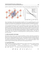
We show a result of simulation in Fig. 1. It can be concluded that the output signal follows
the reference even if disturbances exit in the system.
6. Conclusion
In the responses (Fig. 1) of the discrete time model following control system for nonlinear
descriptor system, the output signal follows the references even though disturbances exit in
the system. The effectiveness of this method has thus been verified. The future topic is that
the case of nonlinear system for 1
γ
≥ will be proved and analysed.
Discrete Time Systems

140

Fig. 1. Responses of the system for nonlinear descriptor system in discrete time
7. References
Wu,S.; Okubo,S.; Wang,D. (2008). Design of a Model Following Control System for
Nonlinear Descriptor System in Discrete Time, Kybernetika, vol.44,no.4,pp.546-556.
Byrnes,C.I; Isidori,A. (1991). Asymptotic stabilization of minimum phase nonlinear system,

IEEE Transactions on Automatic Control, vol.36,no.10,pp.1122-1137.
Casti,J.L. (1985). Nonlinear Systems Theory, Academic Press, London.
Furuta,K. (1989). Digital Control (in Japanese), Corona Publishing Company, Tokyo.
Ishidori,A. (1995). Nonlinear Control Systems, Third edition, Springer-Verlag, New York.
Khalil,H.K. (1992). Nonlinear Systems, MacMillan Publishing Company, New York.
Mita,T. (1984). Digital Control Theory (in Japanese), Shokodo Company, Tokyo.
Mori,Y. (2001). Control Engineering (in Japanese), Corona Publishing Company, Tokyo.
Okubo,S. (1985). A design of nonlinear model following control system with disturbances
(in Japanese), Transactions on Instrument and Control Engineers, vol.21,no.8,pp.792-
799.
Okubo,S. (1986). A nonlinear model following control system with containing inputs in
nonlinear parts (in Japanese), Transactions on Instrument and Control Engineers,
vol.22,no.6,pp.714-716.
Okubo,S. (1988). Nonlinear model following control system with unstable zero points of the
linear part (in Japanese), Transactions on Instrument and Control Engineers,
vol.24,no.9,pp.920-926.
Okubo,S. (1992). Nonlinear model following control system using stable zero assignment (in
Japanese), Transactions on Instrument and Control Engineers, vol.28, no.8, pp.939-946.
Takahashi,Y. (1985). Digital Control (in Japanese), Iwanami Shoten,Tokyo.
Zhang,Y; Okubo,S. (1997). A design of discrete time nonlinear model following control
system with disturbances (in Japanese), Transactions on The Institute of Electrical
Engineers of Japan, vol.117-C,no.8,pp.1113-1118.
Jun Xu
National University of Singapore
Singapore
1. Introduction
Most physical systems have only limited states to be measured and fed back for system
controls. Although sometimes, a reduced-order observer can be designed to meet the
requirements of full-state feedback, it does introduce extra dynamics, which increases the
complexity of the design. This naturally motivates the employment of output feedback, which

only use measurable output in its feedback design. From implementation point of view, static
feedback is more cost effective, more reliable and easier to implement than dynamic feedback
(Khalil, 2002; Kuˇcera & Souza, 1995; Syrmos et al., 1997). Moreover, many other problems are
reducible to some variation of it. Simply stated, the static output feedback problem is to find
a static output feedback so that the closed-loop system has some desirable characteristics, or
determine the nonexistence of such a feedback (Syrmos et al., 1997). This problem, however,
still marked as one important open question even for LTI systems in control engineering.
Although this problem is also known NP-hard (Syrmos et al., 1997), the curious fact to
note here is that these early negative results have not prevented researchers from studying
output feedback problems. In fact, there are a lot of existing works addressing this problem
using different approaches, say, for example, Riccati equation approach, rank-constrained
conditions, approach based on structural properties, bilinear matrix inequality (BMI)
approaches and min-max optimization techniques (e.g., Bara & Boutayeb (2005; 2006); Benton
(Jr.); Gadewadikar et al. (2006); Geromel, de Oliveira & Hsu (1998); Geromel et al. (1996);
Ghaoui et al. (2001); Henrion et al. (2005); Kuˇcera & Souza (1995); Syrmos et al. (1997) and the
references therein). Nevertheless, the LMI approaches for this problem remain popular (Bara
& Boutayeb, 2005; 2006; Cao & Sun, 1998; Geromel, de Oliveira & Hsu, 1998; Geromel et al.,
1996; Prempain & Postlethwaite, 2001; Yu, 2004; Zeˇcevi´c & Šiljak, 2004) due to simplicity and
efficiency.
Motivated by the recent work (Bara & Boutayeb, 2005; 2006; Geromel et al., 1996; Xu & Xie,
2005a;b; 2006), this paper proposes several scaling linear matrix inequality (LMI) approaches
to static output feedback control of discrete-time linear time invariant (LTI) plants. Based on
whether a similarity matrix transformation is applied, we divide these approaches into two
parts. Some approaches with similarity transformation are concerned with the dimension
and rank of system input and output. Several different methods with respect to the system
state dimension, output dimension and input dimension are given based on whether the
distribution matrix of input B or the distribution matrix of output C is full-rank. The other

Output Feedback Control of Discrete-time
LTI Systems: Scaling LMI Approaches

9
approaches apply Finsler’s Lemma to deal with the Lyapunov matrix and controller gain
directly without similarity transformation. Compared with the BMI approach (e.g., Henrion
et al. (2005)) or VK-like iterative approach (e.g.,Yu (2004)), the scaling LMI approaches are
much more efficient and convergence properties are generally guaranteed. Meanwhile, they
can significantly reduce the conservatism of non-scaling method, (e.g.,Bara & Boutayeb (2005;
2006)). Hence, we show that our approaches actually can be treated as alternative and
complemental methods for existing works.
The remainder of this paper is organized as follows. In Section 2, we state the system and
problem. In Section 3, several approaches based on similarity transformation are given. In
Subection 3.1, we present the methods for the case that B is full column rank. Based on
the relationship between the system state dimension and input dimension, we discuss it in
three parts. In Subsection 3.2, we consider the case that C is full row rank in the similar way.
In Subsection 3.3, we propose another formulations based on the connection between state
feedback and output feedback. In Section 4, we present the methods based on Finsler’s lemma.
In Section 5, we compare our methods with some existing works and give a brief statistical
analysis. In Section 6, we extend the latter result to H
∞
control. Finally, a conclusion is given
in the last section. The notation in this paper is standard.
R
n
denotes the n dimensional real
space. Matrix A
> 0(A ≥ 0) means A is positive definite (semi-definite).
2. Problem formulation
Consider the following discrete-time linear time-invariant (LTI) system:
x
(t + 1)=A
o

x(t)+B
o
u( t) (1)
y
(t)=C
o
x(t) (2)
where x
∈R
n
, u ∈R
m
and y ∈R
l
. All the matrices mentioned in this paper are appropriately
dimensioned. m
< n and l < n.
We want to stabilize the system (1)-(2) by static output feedback
u
(t)=Ky(t) (3)
The closed-loop system is
x
(t + 1)=
˜
Ax
(t)=(A
o
+ B
o
KC

o
)x(t) (4)
The following lemma is well-known.
Lemma 1. (Boyd et al., 1994) The closed-loop system (4) is (Schur) stable if and only if either one of
the following conditions is satisfied:
P
> 0,
˜
A
T
P
˜
A − P < 0(5)
Q
> 0,
˜
AQ
˜
A
T
− Q < 0(6)
3. Scaling LMIs with similarity transformation
This section is motivated by the recent LMI formulation of output feedback control (Bara
& Boutayeb, 2005; 2006; Geromel, de Souze & Skelton, 1998) and dilated LMI formulation
(de Oliveira et al., 1999; Xu et al., 2004).
142
Discrete Time Systems
3.1 B
o
with full column-rank

We assume that B
o
is of full column-rank, which means we can always find a non-singular
matrix T
b
such that T
b
B
o
=

I
m
0

. In fact, using singular value decomposition (SVD), we can
obtain such T
b
. Hence the new state-space representation of this system is given by
A
= T
b
A
o
T
−1
b
=

A

11
A
12
A
21
A
22

, B
= T
b
B
o
, C = C
o
T
−1
b
(7)
The closed-loop system (4) is stable if and only if
˜
A
b
= A + BK C is stable
In this case, we divide it into 3 situations: m
= n − m, m < n −m,andm > n −m.Let
P
=

P

11
P
12
P
T
12
P
22

∈R
n×n
, P
11
∈R
m×m
, P
12
∈R
m×(n−m)
(8)
For the third situation, let
P
12
=[P
(1)
12
P
(2)
12
], P

11
=

P
(1)
11
P
(2)
11
P
(2)T
11
P
(3)
11

(9)
where P
(1)
12
∈R
(n−m)×(n−m)
and P
(1)
11
∈R
(n−m)×(n−m)
.
Theorem 1. The discrete-time system (1)-(2) is stabilized by (3) if there exist P
> 0 defined in (8) and

R, such that
⎧
⎨
⎩
Φ
(Θ
1
) < 0, m = n − m
Φ
(Θ
2
) < 0, m < n − m
Φ
(Θ
3
) < 0, m > n − m
(10)
where ε
∈R,
Φ
(Θ
1
)=

A
T
Θ
1
A − P ∗
RC +[P

11
P
12
]A −P
11

< 0 (11)
Θ
1
=

00
0 P
22
+ ε
2
P
11
−εP
12
−εP
T
12

, (12)
Θ
2
=
⎡
⎣

00
0 P
22
−ε

P
12
0

−ε[P
T
12
0]+ε
2

P
11
0
00

⎤
⎦
,
Θ
3
=

00
0 P
22

−εP
(1)T
12
−εP
(1)
12
+ ε
2
P
(1)
11

.
Furthermore, a static output feedback controller gain is given by
K
= P
−1
11
R (13)
Proof: Noting that
(BK C)
T
P(BK C)=C
T
K
T
P
11
KC,
143

Output Feedback Control of Discrete-time LTI Systems: Scaling LMI Approaches
PBKC =

P
11
P
T
12

KC
(5) is equivalent to
([P
11
P
12
]A + P
11
KC)
T
P
−1
11
([P
11
P
12
]A + P
11
KC)
−

A
T

P
11
P
T
12

P
−1
11
[P
11
P
12
]A + A
T
PA −P < 0
(14)
Considering that
P
−

P
11
P
T
12


P
−1
11
[P
11
P
12
]=

00
0 P
22
−P
T
12
P
−1
11
P
12

For the first situation m
= n − m, consider the following inequality:
(P
12
−εP
11
)
T
P

−1
11
(P
12
−εP
11
) ≥ 0 (15)
or equivalently
P
T
12
P
−1
11
P
12
≥ εP
T
12
+ εP
12
−ε
2
P
11
(16)
(14) is equivalent to

A
T

Θ
0
A − P ∗
P
11
KC +[P
11
P
12
]A −P
11

< 0 (17)
where
Θ
0
=

00
0 P
22
− P
T
12
P
−1
11
P
12


Using the fact (16), we have Θ
0
≤ Θ
1
, and consequentially, Φ(Θ
0
) ≤ Φ(Θ
1
). Hence if (11) is
satisfied, (5) is satisfied as well.
For the second situation, let the inequality

P
12
0

−ε

P
11
0
00

T

P
11
0
0 I


−1

P
12
0

−ε

P
11
0
00

≥ 0
(18)
where

P
12
0

∈R
(n−m)×(n−m)
and

P
11
0
0 I


∈R
(n−m)×(n−m)
. Note that (18) is equivalent to
P
T
12
P
−1
11
P
12
≥ ε

P
12
0

T
+ ε

P
12
0

−ε
2

P
11
0

00

(19)
For the third situation, noting that
(

P
12
0

−εP
11
)
T
P
−1
11
(

P
12
0

−εP
11
) ≥ 0 (20)
we have

P
T

12
0

P
−1
11

P
12
0

≥ ε

P
T
12
0

+ ε

P
12
0

−ε
2
P
11
(21)
(21) implies

P
T
12
P
−1
11
P
12
≥ εP
(1)T
12
+ εP
(1)
12
−ε
2
P
(1)
11
(22)
144
Discrete Time Systems
Hence we complete the proof.
Remark 1. If ε
≡ 0 is set , then Theorem 1 recovers the result stated in (Bara & Boutayeb, 2006). We
shall note that ε actually plays an important role in the scaling LMI formulation in Theorem 1. If ε
≡ 0,
Theorem 1 implies A
T
22

P
22
A
22
− P
22
< 0 and P
22
> 0, i.e., the system matrix A
22
must be Schur
stable, which obviously is an unnecessary condition and limits the application of this LMI formulation.
However, with the aid of ε, we relax this constraint. A searching routine, such as fminsearch (simplex
search method) in Matlab
©
, can be applied to the following optimization problem (for a fixed ε,wehave
an LMI problem):
min
ε,P,R
λI, s.t. Φ(Θ) < λI (23)
The conservatism of Theorem 1 lies in these relaxations (15) or (16) on (5). To further relax the
conservatism, we may choose a diagonal matrix
 = diag{ε
1
, , ε
m
}, ε
i
≥ 0, instead of the single
scalar ε. For example,

P
T
12
P
−1
11
P
12
≥ P
T
12
+ P
12
−P
11
 (24)
Then we shall search the optimal value over multiple scalars for (23).
Remark 2. In (Bara & Boutayeb, 2006), a different variable replacement is given:
P
2
= P
22
− P
T
12
P
−1
11
P
12

(25)
in (8). However, it is easily proved that these two transformations actually are equivalent. In fact, in
(8), we have P
11
> 0 and P
2
> 0 since P > 0. Based on (17), we have
⎡
⎣
A
T

00
0 P
2

A
−Λ
0
∗
P
11
KC +[P
11
P
12
]A −P
11
⎤
⎦

< 0 (26)
where
Λ
0
=

P
11
P
12
P
T
12
P
2
+ P
T
12
P
−1
11
P
12

= P (27)
Hence, for the above three situations, we have an alternative condition, which is stated in the
following lemma.
Theorem 2. The discrete-time system (1)-(2) is stabilized by (3) if there exist P
11
> 0,P

2
> 0,P
12
and R with P defined in (27), such that
⎧
⎨
⎩
Υ
(Λ
1
) < 0, m = n −m
Υ
(Λ
2
) < 0, m < n −m
Υ
(Λ
3
) < 0, m > n −m
(28)
where ε
∈R,
Υ
(Λ
i
)=
⎡
⎣
A
T


00
0 P
2

A
−Λ
i
∗
RC +[P
11
P
12
]A −P
11
⎤
⎦
,
Λ
1
=

P
11
P
12
P
T
12
P

2
−ε
2
P
11
+ εP
12
+ εP
T
12

,
145
Output Feedback Control of Discrete-time LTI Systems: Scaling LMI Approaches
Λ
2
=
⎡
⎣
P
11
P
12
P
T
12
P
2
+ ε


P
12
0

+ ε[P
T
12
0] −ε
2

P
11
0
0 I

⎤
⎦
,
Λ
3
=

P
11
P
12
P
T
12
P

2
+ εP
(1)T
12
+ εP
(1)
12
−ε
2
P
(1)
11

.
Furthermore, a static output controller gain is given by (13).
Proof: We only consider the first case. Replacing P
2
and R by P
22
and K using (25) and (13), we
can derive that (28) is a sufficient condition for (5) with the P defined in (8).
3.2 C
o
with full row-rank
When C
o
is full row rank, there exists a nonsingular matrix T
c
such that C
o

T
−1
o
=[I
l
0].
Applying a similarity transformation to the system (1)-(2), the closed-loop system (4) is stable
if and only if
˜
A
c
= A + BK C is stable
where A
= T
c
A
o
T
−1
c
, B = T
c
B
o
and C = C
o
T
−1
c
=[I

l
0].
Similarly to Section 3.1, we can also divide this problem into three situations: l
= n − l,
l
< n − l and l > n − l. Weusethecondition(6)hereandpartitionQ as Q =

Q
11
Q
12
Q
T
12
Q
22

,
where Q
11
∈R
l×l
.
Theorem 3. The discrete-time system (1)-(2) is stabilized by (3) if there exist Q
> 0 and R, such that
⎧
⎨
⎩
Γ
(

¯
Θ
1
) < 0, l = n −l
Γ
(
¯
Θ
2
) < 0, l < n −l
Γ
(
¯
Θ
3
) < 0, l > n −l
(29)
where ε
∈R,
Γ
(
¯
Θ
i
)=

A
¯
Θ
i

A
T
− Q ∗
(
A[Q
11
Q
12
]
T
+ BR)
T
−Q
11

,
¯
Θ
1
=

00
0 Q
22
+ ε
2
Q
11
−εQ
12

−εQ
T
12

,
¯
Θ
2
=
⎡
⎣
00
0 Q
22
+ ε
2

Q
11
0
00

−ε

Q
12
0

−ε[Q
T

12
0]
⎤
⎦
,
¯
Θ
3
=

00
0 Q
22
+ ε
2
Q
(1)
11
−εQ
(1)T
12
−εQ
(1)
12

,
Q
(1)
11
and Q

(1)
12
are properly dimensioned partitions of Q
11
and Q
12
. Furthermore, a static output
feedback controller gain is given by
K
= RQ
−1
11
(30)
146
Discrete Time Systems
Proof: We only prove the first case l = n − l, since the others are similar. Noting that
(BK C)Q(BK C)
T
= BK Q
11
K
T
B and BKCQ = BK [Q
11
Q
12
], (6) is equivalent to
(A[Q
11
Q

12
]
T
+ BK Q
11
)Q
−1
11
(A[Q
11
Q
12
]
T
+ BK Q
11
)
T
−A

Q
11
Q
T
12

Q
−1
11
[Q

11
Q
12
]A
T
+ AQ A
T
− Q < 0
(31)
Using the fact that
Q
−

Q
11
Q
T
12

Q
−1
11
[Q
11
Q
12
]=

00
0 Q

T
12
Q
−1
11
Q
12

we infer that stability of the close-loop system is equivalent to the existing of a Q
> 0such
that

A
¯
Θ
0
A
T
− Q ∗
(
A[Q
11
Q
12
]+BK Q
11
)
T
−Q
11


< 0 (32)
where
¯
Θ
0
=

00
0 Q
22
− Q
T
12
Q
−1
11
Q
12

Since
(Q
12
−εQ
11
)
T
Q
−1
11

(Q
12
−εQ
11
) ≥ 0 (33)
or equivalently,
Q
T
12
Q
−1
11
Q
12
≥ εQ
T
12
+ εQ
12
−ε
2
Q
11
(34)
It follows that (29) implies (32). Hence we complete the proof.
Remark 3. How to compare the conditions in Theorem 3 and Theorem 1 remains a difficult problem.
In the next section, we only give some experiential results based on numerical simulations, which give
some suggestions on the dependence of the results with respect to m and l.
3.3 Transformation-dependent LMIs
The result in this subsection builds a connection between the sets L, K

c
, K
o
,
˜
K
c
and
˜
K
o
,which
are defined as follows. Without causing confusion, we omit the subscript
o
for A
o
, B
o
and C
o
in this subsection.
L = {K ∈R
m×l
:
¯
Astable} (35)
i.e., the set of all admissible output feedback matrix gains;
K
c
= {K

c
∈R
m×n
: A + BK
c
stable} (36)
i.e., the set of all admissible state feedback matrix gains;
K
o
= {K
o
∈R
n×l
: A + K
o
Cstable} (37)
i.e., the set of all admissible observer matrix gains. Based on Lemma 1, we can easily formulate
the LMI solution for sets
K
c
and K
o
. In fact, they are equivalent to following two sets
respectively:
˜
K
c
= {K
c
= W

c2
W
−1
c1
∈R
m×n
: (W
c1
, W
c2
) ∈W
c
}
(38)
147
Output Feedback Control of Discrete-time LTI Systems: Scaling LMI Approaches
and
W
c
= {W
c1
∈R
n×n
, W
c2
∈R
m×n
: W
c1
> 0, Ψ

c
< 0} (39)
where Ψ
c
=

−W
c1
AW
c1
+ BW
c2
W
c1
A
T
+ W
T
c2
B
T
−W
c1

.
˜
K
o
= {K
o

= W
−1
o1
W
o2
∈R
n×l
: (W
o1
, W
o2
) ∈W
o
}
(40)
and
W
o
= {W
o1
∈R
n×n
, W
o2
∈R
n×l
: W
o1
> 0, Ψ
o

< 0}
(41)
where Ψ
o
=

−W
1o
W
o1
A + W
o2
C
A
T
W
o1
+ C
T
W
T
o2
−W
1o

.
Lemma 2.
L = ∅ if and only if
1.
¯

K
c
= K
c

{K
c
: K
c
Y
c
= 0, Y
c
= N(C)} = ∅;or
2.
¯
K
o
= K
o

{K
c
: Y
o
K
o
= 0, Y
o
= N(B


)} = ∅.
In the affirmative case, any K
∈Lcan be rewritten as
1. K
= K
c
QC
T
(CQC
T
)
−1
;or
2. K
=(B
T
PB)
−1
B
T
PK
o
.
where Q
> 0 and P > 0 are arbitrarily chosen.
Proof: The first statement has been proved in Geromel et al. (1996). For complement, we
give the proof of the second statement. The necessity is obvious since K
o
= BK .Nowwe

prove the sufficiency, i.e., given K
o
∈
¯
K
o
,thereexistsaK, such that the constraint K
o
= BK
is solvable. Note that for
∀P > 0, Θ
o
=

B
T
P
Y
T
o

is full rank, where Y
o
= N(B
T
). In fact,
rank
(Θ
o
Y

o
)=rank(

B
T
PY
o
I
n−m

) ≥ n −m.MultiplyingΘ
o
at the both side of K
o
= BK we have

B
T
PK
o
Y
T
o
K
o

=

B
T

PBL
0

Since B
T
PB is invertible, we have K =(B
T
PB)
−1
B
T
PK
0
. Hence, we can derive the result.
Lemma 3.
L = ∅ ifandonlyifthereexistsE
c
∈R
n×(n−l)
or E
o
∈R
n×(n−m)
, such that one of the
following conditions holds:
1. rank
(T
c
=


C
E
T
c

)=nandC(E
c
) = ∅;or
2. rank
(T
o
=

BE
o

)=nandO(E
o
) = ∅.
where
C(E
c
)=W
c

{(W
c1
, W
c2
) : CW

c1
E
c
= 0, W
c2
E
c
= 0}
O(
E
o
)=W
o

{(W
o1
, W
o2
) : B
T
W
o1
E
o
= 0, E
T
o
W
o2
= 0}

In the affirmative case, any K ∈Lcan be rewritten as
1. K
= W
c2
C
T
(CW
c1
C
T
)
−1
;or
2. K
=(B
T
W
o1
B)
−1
B
T
W
o2
.
148
Discrete Time Systems
Proof: We only prove the statement 2, since the statement 1 is similar. For the necessity, if there
exist K
∈L, then it shall satisfy Lemma 1. Now we let

W
o1
= P, W
o2
= PBK
Choose E
o
= P
−1
Y
o
, Y
o
= N(B
T
). It is known that

BE
o

is full rank. Then we have
B
T
W
o1
E = B
T
Y
o
= 0, E

T
W
o2
= Y
T
o
BK = 0
For sufficiency, we assume there exists E
o
such that the statement 2) is satisfied. Notice that
W
o1
> 0 and the item W
o2
in Ψ
o
can be rewritten as W
o1
W
−1
o1
W
o2
.
W
−1
o1
W
o2
= T

o
(T
T
o
W
o1
T
o
)
−1
T
T
o
W
o2
= B(B
T
W
o1
B)
−1
B
T
W
o2
(42)
since T
o
is invertible and B
T

W
o1
E = 0, E
T
W
o2
= 0. Hence, W
−1
o1
W
o2
can be factorized as
BK,whereK
=(B
T
W
o1
B)
−1
B
T
W
o2
. Now we can derive (5) from the fact Ψ
o
< 0. Thus we
complete the proof.
Remark 4. For a given T
o
,sinceT

−1
o
T
o
= I
n
,T
−1
o
B =

I
m
0

and T
−1
o
E =

0
I
n−m

. S imilarly, For
agivenT
c
,CT
−1
c

=

I
l
0

.
Theorem 4.
L = ∅ if and only if there exists T
c
or T
o
, such that one of the following conditions holds:
1.
˜
W
c
= ∅,
˜
W
c
= {
ˆ
W
c1
∈R
n×n
,
ˆ
W

c2
∈R
m×n
:
ˆ
W
c1
> 0, Φ
c
< 0}
(43)
where
ˆ
A
= T
c
AT
−1
c
,
ˆ
B = T
c
B,
ˆ
W
c1
=

W

c11
0
0 W
c22

,
and
ˆ
W
c2
=

W
c21
0

, W
c11
∈R
l×l
, W
c22
∈R
(n−l)×(n−l)
, W
c21
∈R
m×l
,
Φ

c
=

−
ˆ
W
c1
ˆ
A
ˆ
W
c1
+
ˆ
B
ˆ
W
c2
ˆ
W
c1
ˆ
A
T
+
ˆ
W
T
c2
ˆ

B
T
−
ˆ
W
c1

;
2.
˜
W
o
= ∅,
˜
W
o
= {
ˇ
W
o1
∈R
n×n
,
ˇ
W
o2
∈R
n×r
:
ˇ

W
o1
> 0, Φ
o
< 0}
(44)
where
ˇ
A
= T
−1
o
AT
o
,
ˇ
C = CT
o
,
ˇ
W
o1
=

W
o11
0
0 W
o22


,
and
ˇ
W
o2
=

W
o21
0

,
W
o11
∈R
m×m
, W
o22
∈R
(n−m)×(n−m)
, W
o21
∈R
m×r
,
Φ
o
=

−

ˇ
W
o1
ˇ
W
o1
ˇ
A +
ˇ
W
o2
ˇ
C
ˇ
A
T
ˇ
W
o1
+
ˇ
C
T
ˇ
W
T
o2
−
ˇ
W

o1

.
In the affirmative case, any K
∈Lcan be rewritten as
1. K
= W
c21
W
−1
c11
;or
149
Output Feedback Control of Discrete-time LTI Systems: Scaling LMI Approaches
2. K = W
−1
o11
W
o21
.
Proof: We also only consider the statement 2) here. The sufficiency is obvious according to
Lemma 3, hence, we only prove the necessity.
Note that

−
ˇ
W
o1
ˇ
W

o1
ˇ
A +
ˇ
W
o2
ˇ
C
ˇ
A
T
ˇ
W
o1
+
ˇ
C
T
ˇ
W
T
o2
−
ˇ
W
o1

= T
T
o


−W
o1
W
o1
A + W
o2
C
A
T
W
o1
+ C
T
W
T
o2
−W
o1

T
o
where T
o
=

T
o
0
0 T

o

. Hence, we can conclude that
ˇ
W
o1
= T
T
o
W
o1
T
o
,
ˇ
W
02
= T
T
o
W
o2
Since the system matrices also satisfy
B
T
W
o1
E = 0, E
T
W

o2
= 0
which implies
B
T
T
−T
o
ˇ
W
o1
T
−1
o
E = 0, E
T
T
−T
o
ˇ
W
o2
= 0 (45)
Let
ˇ
W
o1
=

W

o11
W
o12
W
T
o12
W
o22

,
ˇ
W
o2
=

W
o21
W
o23

With the conclusion from Remark 4, (45) implies
W
o12
= 0, W
o23
= 0
Hence we have the structural constraints on
ˇ
W
o1

and
ˇ
W
o2
. Using the results of Lemma 3, we
can easily get the controller L. Thus we complete the proof.
Remark 5. The first statements of Lemma 3 and Theorem 4 are corollaries of the results in Geromel,
de Souze & Skelton (1998); G eromel et al. (1996). Based on Theorem 4, we actually obtain a useful
LMI algorithm for output feedback control design of general LTI systems with fixed E
c
and/or E
o
.For
these LTI systems, we can first make a similarity transformation that makes C
=[I 0] (or B
T
=[I 0]).
Then we force the W
c1
and W
c2
(or W
o1
and W
o2
) to be constrained stru cture shown in Theorem
4. If the corresponding LMIs have solution, we may conclude that the output feedback gain exists;
otherwise, we cannot make a conclusion, as the choice of E
c
or E

o
is simply a special case. Thus we
can choose a scaled E
c
or E
o
, i.e., E
c
or E
o
to perform a one-dimensional search, which converts
the LMI condition in Theorem 4 a scaling LMI. For example, Φ
c
in (43) should be changed as Φ
c
=

−
ˆ
W
1c
A
ˆ
W
c1
+ εB
ˆ
W
c2
ˆ

W
c1
A
T
+ ε
ˆ
W
T
c2
B
T
−
ˆ
W
1c

.
All the approaches in this section require similarity transformation, which can be done
by some techniques, such as the singular value decomposition (SVD). However, those
transformations often bring numerical errors, which sometimes leads to some problems for
the marginal solutions. Hence in the next section, using Finsler’s lemma, we introduce some
methods without the pretreatment on system matrices.
150
Discrete Time Systems
4. Scaling LMIs without similarity transformation
Finsler’s Lemma has been applied in many LMI formulations, e.g., (Boyd et al., 1994; Xu
et al., 2004). With the aid of Finsler’s lemma, we can obtain scaling LMIs without similarity
transformation.
Lemma 4. (Boyd et al., 1994) The following expressions are equivalent:
1. x

T
Ax > 0 for ∀x = 0,subjecttoBx= 0;
2. B
⊥T
AB
⊥
> 0,whereB
⊥
is the kernel of B
T
, i.e., B
⊥
B
T
= 0;
3. A
+ σB
T
B > 0, for some scale σ ∈ R;
4. A
+ XB + B
T
X
T
> 0, for some matrix X.
In order to apply Finsler’s lemma, several manipulation on the Lyapunov inequalities should
be done first. Note that the condition (5) actually states V
(x(t)) = x
T
(t)Px(t) > 0and

ΔV
(x)=V(x(t + 1)) −V(x(t)) < 0. The latter can be rewritten as
ξ
T
Pξ < 0, ξ =[x
T
(t) x
T
(t + 1)]
T
, P =

−P 0
0 P

(46)
Define ζ
=[x
T
u
T
]
T
.Itiseasytoverify:
ξ
= M
p
ζ (47)
[K −1]N
p

ζ = 0 (48)
where
M
p
=

I 0
AB

, N
p
=

C 0
0 I

(49)
That is
(46) s.t. (47)-(48) (50)
Now based on the statements 1) and 4) of Finsler’s Lemma, we can conclude that (50) is
equivalent to
M
T
p
PM
p
+ N
T
p


K
T
−I

X
T
+ X

K
−I

N
p
< 0 (51)
for some
X.Nowwelet
X
T
=[ε
˜
Z
T
Z
T
] (52)
where ε is a given real scalar, Z
=[z
T
1
, z

T
2
, ···, z
T
m
]
T
∈R
m×m
and
˜
Z ∈R
n×m
.Notethat
˜
Z is
constructed from Z with n rows drawing from Z, i.e.,
˜
Z
=[z
T
˜
1
, z
T
˜
2
, ···, z
T
˜

n
]
T
,wherez
T
˜
i
,1≤
˜
i ≤ m is a vector from Z.Sincen ≥ m, there are some same vectors in
˜
Z.Nowwedefine
W
= ZK =[w
T
1
, w
T
2
, ···, w
T
m
]
T
(53)
and
˜
W
=
˜

ZK
=[w
T
˜
1
, w
T
˜
2
, ···, w
T
˜
n
]
T
(54)
where w
T
˜
i
,1≤
˜
i
≤ m is a vector from W. Then (51) can be transferred into following LMI:
M
T
p
PM
p
+


ε
(C
T
˜
W
T
+
˜
WC) ∗
WC −ε
˜
Z
T
−(Z
T
+ Z)

< 0 (55)
151
Output Feedback Control of Discrete-time LTI Systems: Scaling LMI Approaches
Since Z
T
+ Z > B
T
PB ≥ 0, Z is invertible, K = Z
−1
W.
Theorem 5. The discrete-time system (1)-(2) is stabilized by (3) if there exist P
> 0 andZ,W,such

that (55) is satisfied for some scalar ε. Furthermore, the controller is given by K
= Z
−1
W.
The conservatism lies in the construction of
˜
Z, which has to be a special structure.
˜
Z can be
further relaxed using a transformation
˜
Z
= ε
ˆ
ZZ,where
ˆ
Z ∈R
n×m
is a given matrix. In
Theorem 5, the condition (5) is applied. Based on the condition (6), we have the following
Lemma.
Theorem 6. The discrete-time system (1)-(2) is stabilized by (3) if there exist Q
> 0 andZ,W,such
that
M
q
QM
T
q
+


ε
(
˜
W
T
B
T
+ B
˜
W) ∗
W
T
B
T
−ε
˜
Z −(Z
T
+ Z)

< 0 (56)
where
M
q
=

IA
0 C


,
Q =

−Q 0
0 Q

(57)
is satisfied for some scalar ε. Furthermore, the controller is given by K
= Z
−1
W.
Proof: The condition (6) can be rewritten as

I
(BK )
T

T
M
q
QM
T
q

I
(BK )
T

< 0 (58)
Since


I
(BK )
T

T

(BK )
−
I

= 0, (58) can be rewritten as

(BK )
−
I

⊥
M
q
QM
T
q

(BK )
−
I

⊥T
< 0 (59)

Now applying Finsler’s lemma, we have
M
q
QM
T
q
+

(BK )
−
I

X + X
T

(BK )
−
I

T
< 0 (60)
for some
X =[ε
˜
ZZ]. Similar to (52), we construct
˜
Z from Z with its columns. Hence we have
(56), which is a sufficient condition for (6). Thus we complete the proof.
Remark 6. The proof of Theorem 6 is based on the equivalence between 1 and 2 of Finsler’s lemma. It
also provides an alterative proof of Theorem 5 if we note that (5) is equivalent to


I
KC

T
M
T
p
PM
p

I
KC

< 0 (61)
Remark 7. Except for the case that m
= 1 for Theorem 5 and l = 1 for Theorem 6, the construction of
˜
Z is a problem to be considered. So far, we have no systematic method for this problem. However, based
on our experience, the choose of different vectors and their sequence do affect the result.
The following simple result is the consequence of the equivalence of 1 and 3 in Finsler’s
Lemma.
152
Discrete Time Systems
Theorem 7. The discrete-time system (1)-(2) i s stabilized by (3) if there exist P > 0 andK,suchthat

−P − ε
¯
A −ε
¯

A
T
+ ε
2
I
¯
A
T
¯
AP
− I

< 0 (62)
where ε
∈R.
Proof: It is obvious that inequality (42) holds subject to
[
¯
A
− I]ξ = 0. Now we apply the
equivalence between 1 and 3 of Finsler’s lemma and obtain
P−σ[
¯
A − I]

¯
A
−I

=


−P − σ
¯
A
T
¯
A σ
¯
A
σ
¯
AP
−σI

< 0 (63)
for some σ
> 0. Note that −
¯
A
T
¯
A < −ε
¯
A
T
−ε
¯
A + ε
2
I, (63) can be implied by


−P + σ(−ε
¯
A
T
−ε
¯
A + ε
2
I) σ
¯
A
T
σ
¯
AP−σI

< 0 (64)
By redefining P as
1
σ
P, we can obtain the result.
Remark 8. Inequality (51) is also equivalent to
M
T
p
PM
p
−σN
T

p

K
T
−I


K
−I

N
p
< 0 (65)
forsomepositivescalarσ.Hence,wehave
M
T
p
˜
PM
p
− N
T
p

K
T
−I


K

−I

N
p
< 0 (66)
where
˜
P =

−
˜
P 0
0
˜
P

,
˜
P
= σ
−1
P. Using the fact that (K − K
0
)
T
(K − K
0
) ≥ 0, we may obtain an
iterative solution from initial condition K
0

,whereK
0
may be gotten from Lemma 5.
5. Comparison and examples
We shall note that the comparisons of some existing methods (Bara & Boutayeb, 2005; Crusius
& Trofino, 1999; Garcia et al., 2001) with the case of ε
= 0 in Theorem 1 has been given in
(Bara & Boutayeb, 2006), where it states that there are many numerical examples for which
Theorem 1 with ε
= 0 works successfully while the methods in (Bara & Boutayeb, 2005;
Crusius & Trofino, 1999; Garcia et al., 2001) do not and vice-versa. It also stands for our
conditions. Hence, in the section, we will only compare these methods introduced above. The
LMI solvers used here are SeDuMi (v1.3) Sturm et al. (2006) and SDPT3 (v3.4) Toh et al. (2006)
with YALMIP Löfberg (2004) as the interface.
In the first example, we will show the advantage of the scaling LMI with ε compared with the
non-scaling ones. In the second example, we will show that different scaling LMI approaches
have different performance for different situations. As a by-product, we will also illustrate the
different solvability of the different solvers.
153
Output Feedback Control of Discrete-time LTI Systems: Scaling LMI Approaches
Example 1. Consider the unstablesystemasfollows.
A
o
=
⎡
⎢
⎢
⎢
⎢
⎣

0.82 0.0576 0.2212 0.8927 0.0678
0.0574 0.0634 0.6254 0.0926 0.9731
0.0901 0.7228 0.5133 0.2925 0.9228
0.6967 0.0337 0.5757 0.8219 0.9587
0.1471 0.6957 0.2872 0.994 0.5632
⎤
⎥
⎥
⎥
⎥
⎦
B
o
=
⎡
⎢
⎢
⎢
⎢
⎣
0.9505 0.2924
0.3182 0.4025
0.2659 0.0341
0.0611 0.2875
0.3328 0.2196
⎤
⎥
⎥
⎥
⎥

⎦
C
o
=

0.5659 0.255 0.5227 0.0038 0.3608
0.8701 0.5918 0.1291 0.3258 0.994

This example is borrowed from (Bara & Boutayeb, 2006), where output feedback controllers
have been designed. For A
22
from A, it has stable eigenvalue. In this paper, we compare the
design problem with the maximum decay rate, i.e.,
max ρ s.t.
˜
A
T
P
˜
A − P < −ρP
Note that in this example, m
< n −m.Withε = 0, i.e., using the method in (Bara & Boutayeb,
2006), we obtain the maximum ρ
= 0.16, while Theorem 1 gives ρ = 0.18 with ε = −0.09.
However, Theorem 5 only obtains a maximum ρ
= 0.03 with a choice of
ˆ
Z =[I
2
I

2
0]
T
.
Note that the solvability heavily depends on the choice of ε. For example, when ε
= 0.09 for
Theorem 1, the LMI is not feasible.
Now we consider a case that A
22
has an unstable eigenvalue. Consider the above example
with slight changes on A
o
A
o
=
⎡
⎢
⎢
⎢
⎢
⎣
0.9495 0.12048 0.14297 0.19192 0.019139
0.8656 0.28816 0.67152 0.01136 0.38651
0.5038 0.46371 0.9712 0.93839 0.42246
0.13009 0.76443 0.47657 0.54837 0.4089
0.34529 0.61187 0.15809 0.46639 0.53536
⎤
⎥
⎥
⎥

⎥
⎦
We can easily verify that A
22
from A has one unstable eigenvalue 1.004. Hence, the method
in (Bara & Boutayeb, 2006) cannot solve it. However, Theorem 1 generates a solution as
K
=

−0.233763 −0.31506
−3.61207 0.376493

. Meanwhile, Theorem 5 also can get a feasible solution for
ε
= −0.1879 and K =

0.9373
−0.4008
1.5244
−0.7974

. Theorem 4 via a standard SVD without scaling
can also obtain K
=

−0.3914 −0.3603
−2.3604 −1.1034

using (43) or K
=


1.4813 0.5720
−3.7203 −1.8693

using (44).
Example 2. We randomly generate 5000 stabilizable and detectable systems of dimension n
=
4(6, 6, 6, 7, 7),m= 2(3, 1, 5, 4, 3) and l = 2(3, 5, 1,3, 4).
154
Discrete Time Systems
T1 T3
SeDuMi 5000 4982
SDPT3 4975 5000
Table 1. Different solvability of different solvers
T1
α
T3 4.2.2
β
6.3.3 6.1.5 6.5.1 7.4.3 7.3.4
YY4999 4999 4994 4996 4998 4998
YN 1 0 2 3 1 1
NY 0 1 4 1 1 1
NN 0 0 0 0 0 0
Super script
γ
: Y (N) means that the problem can (not) be solved by the corresponding theorems. For
example, the value 4 of third row and third column means that in the random 5000 examples, there are 4
cases that cannot be solved by Theorem 1 while can be solved by Theorem 3.
Table 2. Comparison of Theorem 1 and Theorem 3
Hence we can use Theorem 1 and Theorem 3 with ε

= 0 to solve this problem. Note that
different solvers may give different solvability. For example, given n
= 6, m = 3andl = 3,
in a one-time simulation, the result is given in Table 1. Thus in order to partially eliminate
the effect of the solvers, we choose the combined solvability result from two solvers in this
section.
Table 2 shows the comparison of Theorem 1 and Theorem 3. Some phenomenons (the
solvability of Theorem 1 and Theorem 3 depends on the l and m.Whenm
> l,Theorem1
tends to have a higher solvability than Theorem 3. And vise verse.) was observed from these
results obtained using LMITOOLS provided by Matlab is not shown here.
6. Extension to H
∞
synthesis
The aforementioned results can contribute to other problems, such as robust control. In this
section, we extend it to H
∞
output feedback control problem. Consider the following system:
x
(t + 1)=Ax(t)+B
2
u( t)+B
1
w (67)
y
(t)=Cx(t)+Dw (68)
z
(t)=Ex(t)+Fw (69)
We only consider the case that B
2

is with full rank and assume that the system has been
transferred into the form like (7). Using the controller as (3), the closed-loop system is
x
(t + 1)=
ˆ
Ax(t)+
ˆ
Bw
=(A + B
2
KC)x(t)+(B
1
+ B
2
KD)w
(70)
We attempt to design the controller, such that the L
2
gain sup
z
2
w
2
≤ γ.Itshouldbenoted
that all the aforementioned scaling LMI approaches can be applied here. However, we only
choose one similar to Theorem 1.
155
Output Feedback Control of Discrete-time LTI Systems: Scaling LMI Approaches
Theorem 8. The discrete-time system (67)-(69) is stabilized by (3) and satisfies H
∞

,ifthereexista
matrix P
> 0 defined in (8) and R, such that
⎧
⎨
⎩
(Θ
1
) < 0, m = n −m
(Θ
2
) < 0, m < n −m
(Θ
3
) < 0, m > n −m
(71)
where ε
∈R, Θ
i
is defined in Theorem 1,
(Θ
i
)=
⎡
⎢
⎢
⎣
−P
11
RC +[P

11
P
12
]ARD+[P
11
P
12
]B
1
0
∗ A
T
Θ
i
A − PA
T
Θ
i
B
1
E
T
∗∗ B
T
1
Θ
i
B − γIF
T
∗∗ ∗−γI

⎤
⎥
⎥
⎦
(72)
Proof: Following the arguments in Theorem 1, we can see that (71) implies
(Θ
i
)=
⎡
⎣
ˆ
A
T
P
ˆ
A − P
ˆ
A
T
P
ˆ
BE
T
∗
ˆ
B
T
P
ˆ

B − γIF
T
∗∗−γI
⎤
⎦
< 0 (73)
Using bounded real lemma (Boyd et al., 1994), we can complete the proof.
7. Conclusion
In this paper, we have presented some sufficient conditions for static output feedback control
of discrete-time LTI systems. Some approaches require a similarity transformation to convert
B or C to a special form such that we can formulate the design problem into a scaling
LMI problem with a conservative relaxation. Based on whether B or C is full rank, we
consider several cases with respect to the system state dimension, output dimension and
input dimension. These methods are better than these introduced in (Bara & Boutayeb, 2006)
and might achieve statistical advantages over other existing results (Bara & Boutayeb, 2005;
Crusius & Trofino, 1999; Garcia et al., 2001). The other approaches apply Finsler’s lemma
directly such that the Lyapunov matrix and the controller gain can be separated, and hence
gain benefits for the design. All the presented approaches can be extended to some other
problems. Note that we cannot conclude that the approaches presented in this paper is
definitely superior to all the existing approaches, but introduce some alternative conditions
which may achieve better performance than others in some circumstances.
8. References
Bara, G. I. & Boutayeb, M. (2005). static output feedback stabilization with h
∞
performance
for linear discrete-time systems, IEEE Trans. on Automatic Control 50(2): 250–254.
Bara, G. I. & Boutayeb, M. (2006). A new sufficient condition for the output feedback
stabilization of linear discrete-time systems, Technical report, University Louis
Pasteur, France.
Benton(Jr.), R. E. & Smith, D. (1998). Static output feedback stabilization with prescribed

degree of stability, IEEE Trans. on Automatic Control 43(10): 1493–1496.
156
Discrete Time Systems
Boyd, S., Ghaoui, L. E., Feron, E. & Balakrishnan, V. (1994). Linear Matrix Inequalities in System
and Control Theory, Studies in applied mathematics, SIAM.
Cao, Y. & Sun, Y. (1998). Static output feedback simultaneous stabilization: ILMI approach,
International Journal of Control 70(5): 803–814.
Crusius, C. A. R. & Trofino, A. (1999). Sufficient LMI conditions for output feedback control
problems, IEEE Trans. on Automatic Control 44(5): 1053–1057.
de Oliveira, M. C., Bernussou, J. & Geromel, J. C. (1999). A new discrete-time robust stability
condition, Systems and Control Letters 37: 261–265.
Gadewadikar, J., Lewis, F., Xie, L., Kucera, V. & Abu-Khalaf, M. (2006). Parameterization of
all stabilizing H
∞
static state-feedback gains: Application to output-feedback design,
Proc. Conference on Decision and Control.
Garcia, G., Pradin, B. & Zeng, F. (2001). Stabilization of discrete time linear systems by static
output feedback, IEEE Trans. on Automatic Control 46(12): 1954–1958.
Geromel, J. C., de Oliveira, M. C. & Hsu, L. (1998). LMI characterization of structural and
robust stability, Linear Algebra and its Application 285: 69–80.
Geromel, J. C., de Souze, C. C. & Skelton, R. E. (1998). Static output feedback controllers:
stability and convexity, IEEE Trans. on Automatic Control 43(1).
Geromel, J. C., Peres, P. L. D. & Souza, S. R. (1996). Convex analysis of output feedback
control problems: Robust stability and performance, IEEE Trans. on Automatic Control
41(7): 997–1003.
Ghaoui, L. E., Oustry, F. & Aitrami, M. (2001). A cone complementarity linearization algorithm
for static output feedback and related problems, IEEE Trans. on Automatic Control
42(8): 870–878.
Henrion, D., Löfberg, J., Koˇcvara, M. & Stingl, M. (2005). Solving polynomial static output
feedback problems with PENBMI, Proc. Conference on Decision and Control.

Khalil, H. K. (2002). Nonlinear Systems, 3rd edn, Pretince Hall, New Jersey, USA.
Kuˇcera, V. & Souza, C. E. D. (1995). A necessary and sufficient condition for output feedback
stabilizability, Automatica 31(9): 1357–1359.
Löfberg, J. (2004). YALMIP : A toolbox for modeling and optimization in MATLAB, the CACSD
Conference, Taipei, Taiwan.
Prempain, E. & Postlethwaite, I. (2001). Static output feedback stabilisation with H
∞
performance for a class of plants, Systems and Control Letters 43: 159–166.
Sturm, J. F., Romanko, O. & Pólik, I. (2006). Sedumi: http: // sedumi.mcmaster.ca/, User
manual, McMaster University.
Syrmos, V. L., Abdallab, C., Dprato, P. & Grigoriadis, K. (1997). Static output feedback - a
survey, Automatica 33(2): 125–137.
Toh, K. C., Tütüncü, R. H. & Todd, M. J. (2006). On the implementation and usage of SDPT3 - a
MATLAB software package for semidefinite-quadratic-linear programming, version
4.0, Manual, National University of Singapore, Singapore.
Xu, J. & Xie, L. (2005a). H
∞
state feedback control of discrete-time piecewise affine systems,
IFAC World Congress, Prague, Czech.
Xu, J. & Xie, L. (2005b). Non-synchronized H
∞
estimation of discrete-time piecewise linear
systems, IFAC World Congress, Prague, Czech.
Xu, J. & Xie, L. (2006). Dilated LMI characterization and a new stability criterion for polytopic
uncertain systems, IEEE World Congress on Intelligent Control and Automation, Dalian,
China, pp. 243–247.
157
Output Feedback Control of Discrete-time LTI Systems: Scaling LMI Approaches
Xu, J., Xie, L. & Soh, Y. C. (2004). H
∞

and generalized H
2
estimation of continuous-time
piecewise linear systems, the 5th Asian Control Conference, IEEE, Melbourne,
Australia.
Yu, J. (2004). A new static output feedback approach to the suboptimal mixed H
2
\H
∞
problem, Int. J. Robust Nonlinear Control 14: 1023–1034.
Zeˇcevi´c, A. I. & Šiljak, D. D. (2004). Design of robust static output feedback for large-scale
systems, IEEE Trans. on Automatic Control 49(11): 2040–2044.
158
Discrete Time Systems
10
Discrete Time Mixed LQR/H
∞
Control Problems
Xiaojie Xu
School of Electrical Engineering, Wuhan University
Wuhan, 430072,
P. R. China

1. Introduction
This chapter will consider two discrete time mixed LQR/ H
∞
control problems. One is the
discrete time state feedback mixed LQR/
H
∞

control problem, another is the non-fragile
discrete time state feedback mixed LQR/
H
∞
control problem. Motivation for mixed
LQR/
H
∞
control problem is to combine the LQR and suboptimal H
∞
controller design
theories, and achieve simultaneously the performance of the two problems. As is well
known, the performance measure in optimal LQR control theory is the quadratic
performance index, defined in the time-domain as

0
: ( () () () ())
TT
k
JxkQxkukRuk
∞
=
=+
∑
(1)
while the performance measure in
H
∞
control theory is
H

∞
norm, defined in the
frequency-domain for a stable transfer matrix
()
zw
Tz as
[]
max
0,2
() : sup [ ( )]
jw
zw zw
w
Tz Te
π
σ
∞
∈
=
where,
0Q ≥
,0R > ,
max
[]
σ
•
denotes the largest singular value.
The linear discrete time system corresponding to the discrete time state feedback mixed
LQR/
H

∞
control problem is

12
(1) () () ()xk Axk Bwk Buk
+
=+ + (2.a)

112
() () ()zk Cxk D uk=+
(2.b)
with state feedback of the form

() ()uk Kxk
=
(3)
where,
()
n
xk R∈ is the state, ( )
m
uk R∈ is the control input, ( )
q
wk R∈ is the disturbance
input that belongs to
2
[0, )L
∞
,()
p

zk R∈ is the controlled output.
A
,
1
B ,
2
B ,
1
C and
12
D
are known matrices of appropriate dimensions. Let
0
(0)xx
=
.
The closed loop transfer matrix from the disturbance input
w to the controlled output z is
New Trends in Technologies

160
1
() : ( )
0
KK
zw K K K
K
AB
Tz CzIA B
C

−
⎡⎤
==−
⎢⎥
⎣⎦

where,
2
:
K
AABK=+ ,
1
:
K
BB
=
,
112
:
K
CCDK
=
+ .
Recall that the discrete time state feedback optimal LQR control problem is to find an
admissible controller that minimizes the quadratic performance index (1) subject to the
systems (2) (3) with 0
w
=
, while the discrete time state feedback H
∞

control problem is to
find an admissible controller such that
()
zw
Tz
γ
∞
<
subject to the systems (2)(3) for a given
number
0
γ
>
. While we combine the two problems for the systems (2)(3) with
2
[0, )wL∈∞,
the quadratic performance index (1) is a function of the control input
()uk and disturbance
input
()wk
in the case of
(0)x
being given and
γ
being fixed. Thus, it is not possible to pose
a mixed LQR/
H
∞
control problem that is to find an admissible controller that achieves the
minimization of quadratic performance index (1) subject to

()
zw
Tz
γ
∞
<
for the systems
(2)(3) with
2
[0, )wL∈∞
because the quadratic performance index (1) is an uncertain function
depending on the uncertain disturbance input
()wk . In order to eliminate this difficulty, the
design criteria of state feedback mixed LQR/
H
∞
control problem should be replaced by the
design criteria
2
sup inf{ }
K
wL
J
+
∈
subject to
()
zw
Tz
γ

∞
<

because for all
2
[0, )wL
∈
∞ , the following inequality always exists
2
inf{ } sup inf{ }
KK
wL
JJ
+
∈
≤

The stochastic problem corresponding to this problem is the combined LQG/
H
∞
control
problem that was first presented by Bernstein & Haddad (1989). This problem is to find an
admissible fixed order dynamic compensator that minimizes the expected cost function of
the form
lim ( )
TT
t
JxQxuRu
→∞
=Ε + subject to

zw
T
γ
∞
<
.
Here, the disturbance input w of this problem is restricted to be white noise. Since the
problem of Bernstein & Haddad (1989) involves merely a special case of fixing weighting
matrices
Q
and
R , it is considered as a mixed
2
H / H
∞
problem in special case. Doyle et
al. (1989b) considered a related output feedback mixed
2
/HH
∞
problem (also see Doyle et
al., 1994). The two approaches have been shown in Yeh et al. (1992) to be duals of one
another in some sense. Also, various approaches for solving the mixed
2
/HH
∞
problem
are presented (Rotea & Khargonekar , 1991; Khargonekar & Rotea, 1991; Zhou et al., 1994;
Limebeer et al. 1994; Sznaier ,1994; Rotstein & Sznaier, 1998 ; Sznaier et al. , 2000) . How-
ever, no approach has involved the mixed LQR/

H
∞
control problem until the discrete time
state feedback controller for solving this problem was presented by Xu (1996). Since then,
several approaches to the mixed LQR /
H
∞
control problems have been presented in Xu
(2007, 2008).
The first goal of this chapter is to, based on the results of Xu (1996,2007), present the simple
approach to discrete time state feedback mixed LQR /
H
∞
control problem by combining
the Lyapunov method for proving the discrete time optimal LQR control pro-blem with an
Discrete Time Mixed LQR/H
∞
Control Problems

161
extension of the discrete time bounded real lemma, the argument of compl-etion of squares
of Furuta & Phoojaruenchanachi (1990) and standard inverse matrix man-ipulation of Souza
& Xie (1992).
On the other hand, unlike the discrete time state feedback mixed LQR /
H
∞
control
problem, state feedback corresponding to the non-fragile discrete time state feedback mixed
LQR/
H

∞
control problem is a function of controller uncertainty
()FkΔ
, and is given by

ˆ
() ()uk Fxk
∞
=
,
ˆ
()FF Fk
∞∞
=+Δ
(4)
where,
()FkΔ is the controller uncertainty.
The closed-loop transfer matrix from disturbance input w to the controlled output z and
quadratic performance index for the closed-loop system (2) (4) is respectively
ˆˆ
1
ˆˆˆ
ˆ
ˆ
() : ( )
0
FF
zw
FFF
F

AB
Tz CzIA B
C
∞∞
∞
∞∞
∞
−
⎡⎤
⎢⎥
==−
⎢⎥
⎣⎦

and
22
11
2
2
22
0
ˆ
:{ () () }
k
JQxkRuk w
γ
∞
=
=+−
∑

where,
ˆ
2
ˆ
:
F
AABF
∞
∞
=+ ,
ˆ
1
:
F
BB
∞
=
,
ˆ
112
ˆ
:
F
CCDF
∞
∞
=+ , 0
γ
> is a given number.

Note that the feedback matrix
ˆ
F
∞
of the considered closed-loop system is a function of the
controller uncertainty
()Fk
Δ
, this results in that the quadratic performance index (1) is not
only a function of the controller
F
∞
and disturbance input ()wk but also a function of the
controller uncertainty
()Fk
Δ
in the case of (0)x being given and
γ
being fixed. We can
easily know that the existence of disturbance input
()wk and controller uncertainty ()FkΔ
makes it impossible to find
2
sup inf { }
wL K
J
+
∈
, while the existence of controller uncertainty
()FkΔ also makes it difficult to find

2
sup { }
wL
J
+
∈
. In order to eliminate these difficulties, the
design criteria of non-fragile discrete time state feedback mixed LQR/
H
∞
control problem
should be replaced by the design criteria
2
ˆ
sup { }
wL
J
+
∈
subject to ()
zw
Tz
γ
∞
<
.
Motivation for non-fragile problem came from Keel & Bhattacharyya (1997). Keel &
Bhattacharyya (1997) showed by examples that optimum and robust controllers, designed
by using the
2

H
,
H
∞
,
1
l , and
μ
formulations, can produce extremely fragile controllers, in
the sense that vanishingly small perturbations of the coefficients of the designed controller
destabilize the closed-loop system; while the controller gain variations could not be avoided
in most applications.This is because many factors, such as the limitations in available com-
puter memory and word-length capabilities of digital processor and the A/D and D/A
converters,result in the variation of the controller parameters in controller implementation.
Also, the controller gain variations might come about because of external effects such as
temperature changes.Thus, any controller must be insensitive to the above-mentioned con-
toller gain variation. The question arised from this is how to design a controller that is inse-
nsitive, or non-fragile to error/uncertainty in controller parameters for a given plant. This
New Trends in Technologies

162
problem is said to be a non-fragile control problem. Recently, the non-fragile controller
approach has been used to a very large class of control problems (Famularo et al. 2000,
Haddad et al. 2000, Yang et al 2000, Yang et al. 2001 and Xu 2007).
The second aim of this chapter is to, based on the results of Xu (2007), present a non-fragile
controller approach to the discrete-time state feedback mixed LQR/
H
∞
control problem
with controller uncertainty.

This chapter is organized as follows. In Section 2, we review several preliminary results, and
present two extensions of the well known discrete time bounded real lamma. In Section 3,
we define the discrete time state feedback mixed LQR/
H
∞
control problem. Based on this
definition, we present the both Riccati equation approach and state space approach to the
discrete time state feedback mixed LQR/
H
∞
control problem. In Section 4, we intro-duce
the definition of non-fragile discrete time state feedback mixed LQR/
H
∞
control problem,
give the design method of a non-fragile discrete time state feedback mixed LQR /
H
∞

controller, and derive the necessary and sufficient conditions for the existence of this
controller. In Section 5, we give two examples to illustrate the design procedures and their
effectiveness, respectively. Section 6 gives some conclusions.
Throughout this chapter,
T
A denotes the transpose of A ,
1
A
−
denotes the inverse of A ,
T

A
−
is the shorthand for
1
()
T
A
−
,
~
()Gz denotes the conjugate system of
()Gz
and is the
shorthand for
1
()
T
Gz
−
,
2
(,)L
−
∞+∞ denotes the time domain Lebesgue space,
2
[0, )L +∞
denotes the subspace of
2
(,)L
−

∞+∞ ,
2
(,0]L
−
∞ denotes the subspace of
2
(,)L
−
∞+∞ ,
2
L
+
is
the shorthand for
2
[0, )L
+
∞
and
2
L
−
is the shorthand for
2
(,0]L −∞
.
2. Preliminaries
This section reviews several preliminary results. First, we consider the discerete time Riccati
equation and discrete time Riccati inequality, respectively

1
()
T
XAXIRX AQ
−
=
++ (5)
and

1
() 0
T
AXI RX A Q X
−
+
+−< (6)
with 0
T
QQ=≥ and 0
T
RR
=
> .
We are particularly interested in solution s
X of (5) and (6) such that
1
()IRX A
−
+ is stable.
A symmetric matrix

X is said to the stabilizing solution of discrete time Riccati equation (5)
if it satisfies (5) and is such that
1
()IRX A
−
+ is stable. Moreover, for a sufficiently small
constant 0
δ
> , the discrete time Riccati inequality (6) can be rewritten as

1
()
T
XAXIRX AQ I
δ
−
=+ ++ (7)
Based on the above relation, we can say that if a symmetric matrix
X is a stabilizing
solution to the discrete time Riccati equation (7), then it also is a stabilizing solution to the
discrete time Riccati inequality (6). According to the concept of stabilizing solution of
discrete time Riccati equation, we can define the stabilizing solution
X to the discrete time
Riccati inequality (6) as follow: if there exists a symmetric solution
X to the discrete time
Riccati inequality (6) such that
1
()IRX A
−
+

is stable, then it is said to be a stabilizing
solution to the discrete time Riccati inequality (6) .
Discrete Time Mixed LQR/H
∞
Control Problems

163
If A is invertible, the stabilizing solution to the discerete time Riccati equation (5) can be
obtained through the following simplectic matrix

:
TT
TT
ARAQ RA
S
AQ A
−−
−−
⎡
⎤
+−
=
⎢
⎥
−
⎢
⎥
⎣
⎦
(8)

Assume that
S has no eigenvalues on the unit circle, then it must have n eigenvalues in
1
i
λ
< and n in 1
i
λ
> ( 1,2,,, 1,,2innn
=
+""). If n eigenvectors corresponding to n
eigenvalues in
1
i
λ
<
of the simplectic matrix (8) is computed as
i
i
u
v
⎡
⎤
⎢
⎥
⎣
⎦

then a stabilizing solution to the discerete time Riccati equation (5) is given by
[][]

1
11nn
Xv vu u
−
= ""

Secondly, we will introduce the well known discrete time bounded real lemma (see Zhou et
al. , 1996; Iglesias & Glover, 1991; Souza & Xie, 1992) .
Lemma 2.1 (Discrete Time Bounded Real Lemma)
Suppose that 0
γ
> , ()
AB
M
zRH
CD
∞
⎡⎤
=∈
⎢⎥
⎣⎦
, then the following two statements are
equivalent:
i.
()Mz
γ
∞
< .
ii.
There exists a stabilizing solution 0X ≥ (0X > if (,)CAis observable ) to the discrete

time Riccati equation
21
1
()()0
TTTTTT
AXA X AXB CDU BXA DC CC
γ
−−
−
++ ++=
such that
2
1
()0
TT
UI DDBXB
γ
−
=− + > .
In order to solve the two discrete time state feedback mixed LQR/
H
∞
control problems
considered by this chapter, we introduce the following reference system

12
(1) () () ()xk Axk Bwk Buk+= + +
112
11
22

ˆ
0
() () ()
0
CD
I
zk xk uk
I
⎡⎤⎡⎤
⎢⎥⎢⎥
=+
⎡⎤ ⎡⎤
⎢⎥⎢⎥
ΩΩ
⎢⎥ ⎢⎥
⎢⎥⎢⎥
⎣⎦ ⎣⎦
⎣⎦⎣⎦
(9)
where,
0
0
Q
R
⎡⎤
Ω=
⎢⎥
⎣⎦
and
0

()
ˆ
()
()
zk
zk
zk
⎡
⎤
=
⎢
⎥
⎣
⎦
.
The following lemma is an extension of the discrete time bounded real lemma.
Lemma 2.2 Given the system (2) under the influence of the state feedback (3), and suppose
that 0
γ
> , ()
zw
TzRH
∞
∈
; then there exists an admissible controller K such that
()
zw
Tz
γ
∞

<
if there exists a stabilizing solution
0X
∞
≥ to the discrete time Riccati
equation

21
1
0
TTTTT
KK KK KKKK
AXA X AXBU BXA CC Q KRK
γ
−−
∞∞ ∞ ∞
−
++++= (10)