Discrete Time Systems Part 8 pot

Quadratic D Stabilizable Satisfactory Fault-tolerant Control with
Constraints of Consistent Indices for Satellite Attitude Control Systems

199
(
)
22 22
00 max
TT
J
γ
βλ γβ
<+≤ +xPx UPU
Theorem 2: Consider the system (1) and the cost function (7), for the given index (,)qrΦ
and H
∞
norm-bound index
γ
, if there exists symmetric positive matrix
X
, matrix
Y
and
scalars
0( 4 ~ 9)
i
i
ε
>= such that the following linear matrix inequality

()

0
0
0
0
21
2
456
22
*
**
** *
T
T
T
ab
γ
εεε
⎡⎤
−+
⎢⎥
⎢⎥
−
<
⎢⎥
−+ + +
⎢⎥
⎢⎥
⎣⎦
XAXBYΣ
ID

X I I BJB
Σ
(13)
holds, where
()
21
[ ,,,,,,,, ]
T
TTTTTT
=+Σ CXEY XXYYYYYYJ,
1
22 7 4
[,,,
T
diag
ε
ε
−
=−+ −−
Σ
I EJE Q I
111 1
58 6 7 8 9 9
,,,, ,]
ε
εε ε ε ε ε
−−− −
−+ − − − − −IJ J J J IR I. Then for all admissible uncertainties and
possible faults
M , the faulty closed-loop system (6) with satisfactory fault-tolerant

controller
() ()kk==uKx
11
0
()k
−−
MYXx is asymptotically stable with an H
∞
norm-bound
γ
,
and the corresponding closed-loop cost function (7) is with
122
max
()
T
J
λ
γβ
−
≤+UX U .
According to Theorem 1 and 2, the consistency of the quadratic D stabilizability constraint,
H
∞
performance and cost function indices for fault-tolerant control is deduced as the
following optimization problem.
Theorem 3: Given quadratic D stabilizability index (,)qr
Φ
, suppose the system (1) is robust
fault-tolerant state feedback assignable for actuator faults case, then LMIs (10), (13) have a

feasible solution. Thus, the following minimization problem is meaningful.

(
)
(
)
min : , , ,
i
γ
γε
XY
S.t. LMIs (10), (13) (14)
Proof: Based on Theorem 1, if the system (1) is robust fault-tolerant state feedback
assignable for actuator faults case, then inequality
0
T
CC
−<APA P
has a feasible solution
P , K . And existing 0
λ
> , 0
δ
> , the following inequality holds

0
TTT
CC CC
λδ
⎡⎤

−
+++ +<
⎣⎦
A PA P C C Q K MRMK I (15)
Then existing a scalar
0
γ
, when
0
γ
γ
> , it can be obtained that
(
)
1
2
111
TTT
CC
γ
δ
−
−
<APD I DPD DPA I

where
1
λ
=PP. Furthermore, it follows that
(

)
0
1
2
11 1 1 1
TTTTTT
CC CC C C
γ
−
−
+++ + − <A P A P C C Q K MRMK A P D I D P D D P A
Using Schur complement and Theorem 2, it is easy to show that the above inequality is
equivalent to linear matrix inequality (13), namely,
1
P , K ,
γ
is a feasible solution of LMIs
Discrete Time Systems

200
(10), (13). So if the system (1) is robust fault-tolerant state feedback assignable for actuator
faults case, the LMIs (10), (13) have a feasible solution and the minimization problem (14) is
meaningful. The proof is completed.
Suppose the above minimization problem has a solution
L
X ,
L
Y ,
iL
ε

,
L
γ
, and then any
index
L
γ
γ
> , LMIs (10), (13) have a feasible solution. Thus, the following optimization
problem is meaningful.
Theorem 4: Consider the system (1) and the cost function (7), for the given quadratic D
stabilizability index
(,)qr
Φ
and H
∞
norm-bound index
L
γ
γ
> , if there exists symmetric
positive matrix
X
, matrix
Y
and scalars
0( 1 ~ 9)
i
i
ε

>=
such that the following
minimization

22
min
λ
γβ
+ (16)
S.t. (i) (10), (13)
(ii)
0
T
λ
⎡⎤
−
<
⎢⎥
−
⎢⎥
⎣
⎦
IU
UX

has a solution
min min min min
,, ,
i
ελ

XY , then for all admissible uncertainties and possible faults
M
,
11
0minmin
() () ()kk k
−−
==uKxMYXx
is an optimal guaranteed cost satisfactory fault-tolerant
controller, so that the faulty closed-loop system (6) is quadratically D stabilizable with an H
∞

norm-bound
γ
, and the corresponding closed-loop cost function (7) satisfies
22
min
J
λ
γβ
≤+
.
According to Theorem 1~4, the following satisfactory fault-tolerant controller design
method is concluded for the actuator faults case.
Theorem 5: Given consistent quadratic D stabilizability index (,)qr
Φ
, H
∞
norm index
L

γ
γ
> and cost function index
*22
min
J
λ
γβ
>+ , suppose that the system (1) is robust fault-
tolerant state feedback assignable for actuator faults case. If LMIs (10), (13) have a feasible
solution
X , Y , then for all admissible uncertainties and possible faults M ,
11
0
() () ()kk k
−−
==uKxMYXx is satisfactory fault-tolerant controller making the faulty closed-
loop system (6) satisfying the constraints (a), (b) and (c) simultaneously.
In a similar manner to the Theorem 5, as for the system (1) with quadratic D stabilizability,
H
∞
norm and cost function requirements in normal case, i.e.,
=
MI, we can get the
satisfactory normal controller without fault tolerance.
4. Simulative example
Consider a satellite attitude control uncertain discrete-time system (1) with parameters as
follows:
[]
22 11 0.1 10 10

, , 0.2 0.3 , , , , 0.1, 0.2 .
24 01 0.5 01 01
ab
−
⎡ ⎤ ⎡⎤ ⎡⎤ ⎡⎤ ⎡⎤
=== =====
⎢ ⎥ ⎢⎥ ⎢⎥ ⎢⎥ ⎢⎥
⎣ ⎦ ⎣⎦ ⎣⎦ ⎣⎦ ⎣⎦
ABC DQR

Suppose the actuator failure parameters
{0.4, 0.6}
l
diag
=
M , {1.3, }
u
diag
=
1 . 1M . Given the
quadratic D stabilizability index
(0.5,0.5)
Φ
, we can obtain state-feedback satisfactory fault-
tolerant controller (SFTC), such that the closed-loop systems will meet given indices
constraints simultaneously based on Theorem 5.
Quadratic D Stabilizable Satisfactory Fault-tolerant Control with
Constraints of Consistent Indices for Satellite Attitude Control Systems

201

SFTC
0.5935 3.0187
6.7827 5.6741
⎡
⎤
=
⎢
⎥
−−
⎣
⎦
K

In order to compare, we can obtain the state-feedback satisfactory normal controller (SNC)
without fault-tolerance.
SNC
0.4632 2.4951
5.4682 4.9128
⎡
⎤
=
⎢
⎥
−−
⎣
⎦
K

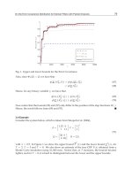
Through simulative calculation, the pole-distribution of the closed-loop system by
satisfactory fault-tolerant controller and normal controller are illustrated in Figure 1, 2 and 3

for normal case and the actuator faults case respectively. It can be concluded that the poles
of closed-loop system driven by normal controller lie in the circular disk Φ(0.5,0.5) for
normal case (see Fig. 1). However, in the actuator failure case, the closed-loop system with
normal controller is unstable; some poles are out of the given circular disk (see Fig. 2). In the
contrast, the performance by satisfactory fault-tolerant controller still satisfies the given pole
index (see Fig. 3). Thus the poles of closed-loop systems lie in the given circular disk by the
proposed method.

0 0.2 0.4 0.6 0.8 1
-0.5
-0.4
-0.3
-0.2
-0.1
0
0.1
0.2
0.3
0.4
0.5

Fig. 1. Pole-distribution under satisfactory normal control without faults
5. Conclusion
Taking the guaranteed cost control in practical systems into account, the problem of
satisfactory fault-tolerant controller design with quadratic D stabilizability and H
∞
norm-
bound constraints is concerned by LMI approach for a class of satellite attitude systems
subject to actuator failures. Attention has been paid to the design of state-feedback controller
that guarantees, for all admissible value-bounded uncertainties existing in both the state and

control input matrices as well as possible actuator failures, the closed-loop system to satisfy
Discrete Time Systems

202
the pre-specified quadratic D stabilizability index, meanwhile the H
∞
index and cost
function are restricted within the chosen upper bounds. So, the resulting closed-loop system
can provide satisfactory stability, transient property, H
∞
performance and quadratic cost
performance despite of possible actuator faults. The similar design method can be extended
to sensor failures case.

-0.2 0 0.2 0.4 0.6 0.8 1 1.2
-0.5
-0.4
-0.3
-0.2
-0.1
0
0.1
0.2
0.3
0.4
0.5

Fig. 2. Pole-distribution under satisfactory normal control with faults

0 0.2 0.4 0.6 0.8 1

-0.5
-0.4
-0.3
-0.2
-0.1
0
0.1
0.2
0.3
0.4
0.5

Fig. 3. Pole-distribution under satisfactory fault-tolerant control with faults
Quadratic D Stabilizable Satisfactory Fault-tolerant Control with
Constraints of Consistent Indices for Satellite Attitude Control Systems

203
6. Acknowledgement
This work is supported by the National Natural Science Foundation of P. R. China under
grants 60574082, 60804027 and the NUST Research Funding under Grant 2010ZYTS012.
7. Reference
H. Yang, B. Jiang, and M. Staroswiecki. Observer-based fault-tolerant control for a class of
switched nonlinear systems, IET Control Theory Appl, Vol. 1, No. 5, pp. 1523-1532,
2007.
D. Ye, and G. Yang. Adaptive fault-tolerant tracking control against actuator faults with
application to flight control, IEEE Trans. on Control Systems Technology, Vol. 14,
No. 6, pp. 1088-1096, 2006.
J. Lunze, and T. Steffen. Control reconfiguration after actuator failures using disturbance
decoupling methods, IEEE Trans. on Automatic Control, Vol. 51, No. 10, pp. 1590-
1601, 2006.

Y. Wang, D. Zhou, and F. Gao. Iterative learning fault-tolerant control for batch processes,
Industrial & Engineering Chemistry Research, Vol. 45, pp. 9050-9060, 2006.
M. Zhong, H. Ye, S. Ding, et al. Observer-based fast rate fault detection for a class of
multirate sampled-data systems, IEEE Trans. on Automatic Control, Vol. 52, No. 3,
pp. 520-525, 2007.
G. Zhang, Z. Wang, X. Han, et al. Research on satisfactory control theory and its application
in fault-tolerant technology, Proceedings of the 5th World Congress on Intelligent
Control and Automation, Hangzhou China, June 2004, Vol. 2, pp. 1521-1524.
D. Zhang, Z. Wang, and S. Hu. Robust satisfactory fault-tolerant control of uncertain linear
discrete-time systems: an LMI approach, International Journal of Systems Science,
Vol. 38, No. 2, pp. 151-165, 2007.
F. Wang, B. Yao, and S. Zhang. Reliable control of regional stabilizability for linear systems,
Control Theory & Applications, Vol. 21, No. 5, pp. 835-839, 2004.
F. Yang, M. Gani, and D. Henrion. Fixed-order robust H
∞
controller design with regional
pole assignment, IEEE Trans. on Automatic Control, Vol. 52, No. 10, pp. 1959-1963,
2007.
A. Zhang, and H. Fang. Reliable H
∞
control for nonlinear systems based on fuzzy control
switching, Proceedings of the 2007 IEEE International Conference on Mechatronics
and Automation, Harbin China, Aug. 2007, pp. 2587-2591.
F. Yang, Z. Wang, D. W.C.Ho, et al. Robust H
∞
control with missing measurements and time
delays, IEEE Trans. on Automatic Control, Vol. 52, No. 9, pp. 1666-1672, 2007.
G. Garcia. Quadratic guaranteed cost and disc pole location control for discrete-time
uncertain systems, IEE Proceedings: Control Theory and Applications, Vol. 144,
No. 6, pp. 545-548, 1997.

X. Nian, and J. Feng. Guaranteed-cost control of a linear uncertain system with multiple
time-varying delays: an LMI approach, IEE Proceedings: Control Theory and
Applications, Vol. 150, No. 1, pp. 17-22, 2003.
J. Liu, J. Wang, and G. Yang. Reliable robust minimum variance filtering with sensor
failures, Proceeding of the 2001 American Control Conference, Arlington USA, Vol.
2, pp. 1041-1046.
Discrete Time Systems

204
H. Wang, J. Lam, S. Xu, et al. Robust H
∞
reliable control for a class of uncertain neutral delay
systems, International Journal of Systems Science, Vol. 33, pp. 611-622, 2002.
G. Yang, J. Wang, and Y. Soh. Reliable H
∞
controller design for linear systems, Automatica,
Vol. 37, pp. 717-725, 2001.
Q. Ma, and C. Hu. An effective evolutionary approach to mixed H
2
/H
∞
filtering with
regional pole assignment, Proceedings of the 6th World Congress on Intelligent
Control and Automation, Dalian China, June 2006, Vol. 2, pp. 1590-1593.
Y. Yang, G. Yang, and Y. Soh. Reliable control of discrete-time systems with actuator
failures, IEE Proceedings: Control Theory and Applications, Vol. 147, No. 4, pp.
428-432, 2000.
L. Yu. An LMI approach to reliable guaranteed cost control of discrete-time systems with
actuator failure, Applied Mathematics and Computation, Vol. 162, pp. 1325-1331,
2005.

L. Xie. Output feedback H
∞
control of systems with parameter uncertainty, International
Journal of Control, Vol. 63, No. 4, pp. 741-750, 1996.
Part 3
Discrete-Time Adaptive Control

Chenguang Yang
1
and Hongbin Ma
2
1
University of Plymouth
2
Beijing Institute of Technology
1
United Kingdom
2
China
1. Introduction
Nowadays nearly all the control algorithms are implemented digitally and consequently
discrete-time systems have been receiving ever increasing attention. However, as to the
development of nonlinear adaptive control methods, which are generally regarded as smart
ways to deal with system uncertainties, most researches are conducted for continuous-time
systems, such that it is very difficult or even impossible to directly apply many well
developed methods in discrete-time systems, due to the fundamental difference between
differential and difference equations for modeling continuous-time and discrete-time systems,
respectively. Even some concepts for discrete-time systems have very different meaning from
those for continuous-time systems, e.g., the “relative degrees” defined for continuous-time
and discrete-time systems have totally different physical explanations Cabrera & Narendra

(1999). Therefore, nonlinear adaptive control of discrete-time systems needs to be further
investigated.
On the other hand, the early studies on adaptive control were mainly concerning on the
parametric uncertainties, i.e., unknown system parameters, such that the designed control
laws have limited robustness properties, where minute disturbances and the presence of
nonparametric model uncertainties can lead to poor performance and even instability of
the closed-loop systems Egardt (1979); Tao (2003). Subsequently, robustness in adaptive
control has been the subject of much research attention for decades. However, due to
the difficulties associated with discrete-time uncertain nonlinear system model, there are
only limited researches on robust adaptive control to deal with nonparametric nonlinear
model uncertainties in discrete-time systems. For example, in Zhang et al. (2001), parameter
projection method was adopted to guarantee boundedness of parameter estimates in presence
of small nonparametric uncertainties under certain wild conditions. For another example,
the sliding mode method has been incorporated into discrete-time adaptive control Chen
(2006). However, in contrast to continuous-time systems for which a sliding mode controller
can be constructed to eliminate the effects of the general uncertain model nonlinearity, for
discrete-time systems, the uncertain nonlinearity is normally required to be of small growth
rate or globally bounded, but sliding mode control is yet not able to completely compensate
for the effects of nonlinear uncertainties in discrete-time. As a matter of fact, unlike in
continuous-time systems, it is much more difficulty in discrete-time systems to deal with

Discrete-Time Adaptive Predictive Control
with Asymptotic Output Tracking
13
nonlinear uncertainties. When the size of the uncertain nonlinearity is larger than a certain
level, even a simple first-order discrete-time system cannot be globally stabilized Xie & Guo
(2000). In an early work on discrete-time adaptive systems, Lee (1996) it is also pointed
out that when there is large parameter time-variation, it may be impossible to construct
a global stable control even for a first order system. Moreover, for discrete-time systems,
most existing robust approaches only guarantee the closed-loop stability in the presence of

the nonparametric model uncertainties, but are not able to improve control performance by
complete compensation for the effect of uncertainties.
Towards the goal of complete compensation for the effect of nonlinear model uncertainties
in discrete-time adaptive control, the methods using output information in previous steps
to compensate for uncertainty at current step have been investigated in Ma et al. (2007)
for first order system, and in Ge et al. (2009) for high order strict-feedback systems. We
will carry forward to study adaptive control with nonparametric uncertainty compensation
for NARMA system (nonlinear auto-regressive moving average), which comprises a general
nonlinear discrete-time model structure and is one of the most frequently employed form in
discrete-time modeling process.
2. Problem formulation
In this chapter, NARMA system to be studied is described by the following equation
y
(k + n)=
n
∑
i=1
θ
T
i
φ
i
(y
(k + n −i)) +
m
∑
j=1
g
j
u(k − m + j)+ν(z( k − τ)) (1)

where y
(k) and u(k) are output and input, respectively. Here
y
(k)=[y(k ), y(k −1), ,y(k −n + 1)]
T
(2)
u
(k)=[u(k −1), u(k −2), ,u(k −m + 1)]
T
(3)
and z
(k)=[y
T
(k), u
T
(k − 1)]
T
.Andfori = 1, 2, ···, n, φ
i
(·) : R
n
→ R
p
i
are known
vector-valued functions, θ
T
i
=[θ
i,1

, ,θ
i,p
i
],andg
j
are unknown parameters. And the last
term ν
(z(k − τ)) represents the nonlinear model uncertainties (which can be regarded as
unmodeled dynamics uncertainties) with unknown time delay τ satisfying 0
≤ τ
min
≤ τ ≤
τ
max
for known constants τ
min
and τ
max
. The control objective to make sure the boundedness
of all the closed-loop signals while to make the output y
(k) asymptotically track a given
bounded reference y
∗
(k).
Time delay is an active topic of research because it is frequently encountered in engineering
systems to be controlled Kolmanovskii & Myshkis (1992). Of great concern is the effect
of time delay on stability and asymptotic performance. For continuous-time systems
with time delays, some of the useful tools in robust stability analysis have been well
developed based on the Lyapunov’s second method, the Lyapunov-Krasovskii theorem and
the Lyapunov-Razumikhin theorem. Following its success in stability analysis, the utility

of Lyapunov-Krasovskii functionals were subsequently explored in adaptive control designs
for continuous-time time delayed systems Ge et al. (2003; 2004); Ge & Tee (2007); Wu (2000);
Xia et al. (2009); Zhang & Ge (2007). However, in the discrete-time case there dos not exist
a counterpart of Lyapunov-Krasovskii functional. To resolve the difficulties associated with
unknown time delayed states and the nonparametric nonlinear uncertainties, an augmented
208
Discrete Time Systems
states vector is introduced in this work such that the effect of time delays can be canceled at
the same time when the effects of nonlinear uncertainties are compensated.
In the NARMA system described in (1), we can see that there is a “relative degree” n which
can be regarded as response delay from input to output. Thus, the control input at the kth
step, u
(k), will actually only determine the output at n-step ahead. The n-step ahead output
y
(k + n) also depends on the following future outputs:
y
(k + 1), y(k + 2), ,y(k + n −2), y(k + n −1) (4)
and ideally the controller should also incorporate the information of these states. However,
dependence on these future states will make the controller non-causal!
If system (1) is linear, e.g., there is no nonlinear functions φ
i
, we could find a so called
Diophantine function by using which system (1) can be transformed into an n-step predictor
where y
(k + n) only depends on outputs at or before the k-th step. Then, linear adaptive
control can be designed under certainty equivalence principal to emulate a deadbeat controller,
which forces the n-step ahead future output to acquire a desired reference value. However,
transformation of the nonlinear system (1) into an n-step predictor form would make the
known nonlinear functions and unknown parameters entangled together and thus not
identifiable. Thus, we propose future outputs prediction, based on which adaptive control can

be designed properly.
Throughout this chapter, the following notations are used.
•
·denotes the Euclidean norm of vectors and induced norm of matrices.
• Z
+
t
represents the set of all integers which are not less than a given integer t.
• 0
[q]
stands for q-dimension zero vector.
• A :
= B means that A is defined as B.
•
(ˆ) and (˜) denote the estimates of unknown parameters and estimate errors, respectively.
3. Assumptions and preliminaries
Some reasonable assumptions are made in this section on the system (1) to be studied. In
addition, some useful lemmas are introduced in this section to facilitate the later control
design.
Assumption 3.1. In system (1), the functional uncertainty ν
(·), satisfies Lipschitz condition, i.e.,
ν(ε
1
) − ν(ε
2
)≤L
ν
ε
1
− ε

2
, ∀ε
1
, ε
2
∈ R
n
,whereL
ν
< λ
∗
with λ
∗
being a small number
defined in (58). The system functions φ
i
(·),i= 1,2, ,n, are also Lipschitz functions with Lipschitz
coefficients L
j
.
Remark 3.1. Any continuously derivable function is Lipschitz on a compact set, refer to Hirsch &
Smale (1974) and any function with bounded derivative is globally Lipschitz. As our objective is
to achieve global asymptotic stability, it is not stringent to assume that the non linearity is globally
Lipschitz.
In fact, Lipschitz condition is a common assumption for nonlinearity in the control community
Arcak et al. (2001); Neši´c & Laila (July, 2002); Neši´c & Teel (2006); Sokolov (2003). In addition, it
is usual in discrete-time control to assume that the uncertain nonlinearity is of small Lipschitz
coefficient Chen et al. (2001); Myszkorowski (1994); Zhang et al. (2001); Zhu & Guo (2004).
When the Lipschitz coefficient is large, discrete-time uncertain systems are not stabilizable as
indicated in Ma (2008); Xie & Guo (2000); Zhang & Guo (2002). Actually, if the discrete-time

209
Discrete-Time Adaptive Predictive Control with Asymptotic Output Tracking
models are derived from continuous-time models, the growth rate of nonlinear uncertainty
can always be made sufficient small by choosing sufficient small sampling time.
Assumption 3.2. In system (1), the control gain coefficient g
m
of current instant control input u(k)
is bounded away from zero, i.e., there is a known constant g
m
> 0 such that |g
m
| > g
m
, and its sign is
known a priori. Thus, without loss of generality, we assume g
m
> 0.
Remark 3.2. It is called unknown control direction problem when the sign of the control gain is
unknown. The unknown control direction problem of n onlinear discrete-time system has been well
addressed in Ge et al. (2008); Yang et al. (2009) but it is out the scope of this chapter.
Definition 3.1. Chen & Narendra (2001) Let x
1
(k) and x
2
(k) be two discrete-time scalar or vector
signals,
∀k ∈ Z
+
t
,foranyt.

•Wedenotex
1
(k)=O[x
2
(k)], if there exist positive constants m
1
,m
2
and k
0
such that x
1
(k)≤
m
1
max
k

≤k
x
2
(k

) + m
2
, ∀k > k
0
.
•Wedenotex
1

(k)=o[x
2
(k)], if there exists a discrete-time function α(k) satisfying lim
k→∞
α(k)=
0 and a constant k
0
such that x
1
(k)≤α(k) max
k

≤k
x
2
(k

), ∀k > k
0
.
•Wedenotex
1
(k) ∼ x
2
(k) if they satisfy x
1
(k)=O[x
2
(k)] and x
2

(k)=O[x
1
(k)].
Assumption 3.3. The input and output of system (1) satisfy
u
(k)=O[y(k + n)] (5)
Assumption 3.3 implies that the system (1) is bounded-output-bounded-input (BOBI) system
(or equivalently minimum phase for linear systems).
For convenience, in the followings we use O
[1] and o[1] to denote bounded sequences and
sequences converging to zero, respectively. In addition, if sequence y
(k) satisfies y(k)=
O[x(k)] or y(k)=o[x(k)],thenwemaydirectlyuseO[x(k)] or o[x(k)] to denote sequence
y
(k) for convenience.
According to Definition 3.1, we have the following proposition.
Proposition 3.1. According to the definition on signal orders in Definition 3.1, we have following
properties:
(i) O
[x
1
(k + τ)] + O[x
1
(k)] ∼ O[x
1
(k + τ)], ∀τ ≥ 0.
(ii) x
1
(k + τ)+o[x
1

(k)] ∼ x
1
(k + τ), ∀τ ≥ 0.
(iii) o
[x
1
(k + τ)] + o[x
1
(k)] ∼ o[x
1
(k + τ)], ∀τ ≥ 0.
(iv) o
[x
1
(k)] + o[x
2
(k)] ∼ o[|x
1
(k)| + |x
2
(k)|].
(v) o
[O[x
1
(k)]] ∼ o[x
1
(k)] + O[1].
(vi) If x
1
(k) ∼ x

2
(k) and lim
k→∞
x
2
(k) = 0,then lim
k→∞
x
1
(k) = 0.
(vii) If x
1
(k)=o[x
1
(k)] + o[1],thenlim
k→∞
x
1
(k) = 0.
(viii) Let x
2
(k)=x
1
(k)+o[x
1
(k)].Ifx
2
(k)=o[1],thenlim
k→∞
x

1
(k) = 0.
Proof. See Appendix A.
Lemma 3.1. Goodwin et al. (1980) (Key Technical Lemma) For some given real scalar sequences s(k),
b
1
(k),b
2
(k) and vector sequence σ(k), if the following conditions hold:
210
Discrete Time Systems
(i) lim
k→∞
s
2
(k)
b
1
(k)+b
2
(k)σ
T
(k)σ(k)
= 0,
(ii) b
1
(k)=O[1] and b
2
(k)=O[1],
(iii) σ

(k)=O[s(k)].
Then, we have
a) lim
k→∞
s(k)=0,andb)σ(k) is bounded.
Lemma 3.2. Define
Z
(k)=[z(k −τ
max
), ,z(k − τ), ,z(k − τ
min
)] (6)
and
l
k
= arg min
l≤k−n
Z(k) − Z(l) (7)
such that
Z
(l
k
)=[z(l
k
−τ
max
), ,z(l
k
−τ), ,z(l
k

−τ
min
)] (8)
and
ΔZ
(k)=Z(k) − Z(l
k
) (9)
Then, if
Z(k) is bounded we have ΔZ(k)→0 as well as ν( z(k − τ)) −ν(z(l
k
−τ))→0.
Proof. Given the definition of l
k
in (7), it has been proved in Ma (2006); Xie & Guo (2000) that
the boundedness of sequence Z
(k) leads to ΔZ(k)→0. As 0 ≤ν(z(k − τ)) − ν(z(l
k
−
τ))≤ΔZ(k), it is obvious that ν(z(k −τ)) −ν(z(l
k
−τ))→0ask → ∞.
According to the definition of ΔZ(k) in (9) and Assumption 3.1, we see that
|ν(z(k −τ)) −ν(z(l
k
−τ))|≤L
ν
ΔZ(k)) (10)
The inequality above serves as a key to compensate for the nonparametric uncertainty, which
will be demonstrated later.

4. Future output prediction
In this section, an approach to predict the future outputs in (4) is developed to facilitate control
design in next section. To start with, let us define an auxiliary output as
y
a
(k + n −1)=
n
∑
i=1
θ
T
i
φ
i
(y(k + n − i)) + ν( z(k − τ)) (11)
such that (1) can be rewritten as
y
(k + n)=y
a
(k + n −1)+
m
∑
j=1
g
j
u(k − m + j) (12)
It is easy to show that
y
a
(k + n − 1)=y

a
(k + n −1) −y
a
(l
k
+ n −1)+y
a
(l
k
+ n −1)
=
n
∑
i=1
θ
T
i
[φ
i
(y(k + n −i)) −φ
i
(y(l
k
+ n −i ))] −
m
∑
j=1
g
j
u(l

k
−m + j)
+
y(l
k
+ n)+(ν(z(k −τ)) −ν(z(l
k
−τ)) (13)
211
Discrete-Time Adaptive Predictive Control with Asymptotic Output Tracking
For convenience, we introduce the following notations
Δφ
i
(k + n −i)=φ
i
(y(k + n − i)) −φ
i
(y(l
k
+ n −i )) (14)
Δu
(k − m + j)=u( k − m + j) −u(l
k
−m + j)
Δν(k − τ)=ν(z(k −τ)) −ν(z(l
k
−τ)) (15)
for i
= 1,2, ,n and j = 1, 2, . . . , m.
Combining (12) and (13), we obtain

y(k + n)=
n
∑
i=1
θ
T
i
Δφ
i
(k + n −i)+
m
∑
j=1
g
j
Δu(k −m + j)+y(l
k
+ n)+Δν(k −τ) (16)
Step 1:
Denote
ˆ
θ
i
(k) and
ˆ
g
j
(k) as the estimates of unknown parameters θ
i
and g

j
at the kth step,
respectively. Then, according to (16), one-step ahead future output y
(k + 1) can be predicted
at the kth step as
ˆ
y
(k + 1|k)=
n
∑
i=1
ˆ
θ
T
i
(k −n + 2)Δφ
i
(k −i + 1)+
m
∑
j=1
ˆ
g
j
(k − n + 2)Δu(k −m + j −n + 1)
+
y(l
k−n+1
+ n) (17)
Now, based on

ˆ
y
(k + 1|k),wedefine
Δ
ˆ
φ
1
(k + 1|k)=φ
1
(
ˆ
y
(k + 1|k)) −φ
1
(y(l
k−n+2
+ n −1)) (18)
which will be used in next step for prediction of two-step ahead output and where
ˆ
y
(k + 1|k)=[
ˆ
y
(k + 1|k), y(k), ,y(k − n + 2)]
T
(19)
Step 2: By using the estimates
ˆ
θ
i

(k) and
ˆ
g
j
(k) and according to (16), the two-step ahead future
output y
(k + 2) can be predicted at the kth step as
ˆ
y
(k + 2|k)=
ˆ
θ
T
1
(k −n + 3)Δ
ˆ
φ
1
(k + 1|k)+
n
∑
i=2
ˆ
θ
T
i
(k −n + 3)Δφ
i
(k −i + 2)
+

m
∑
j=1
ˆ
g
j
(k −n + 3)Δu(k − m + j − n + 2)+y(l
k−n+2
+ n) (20)
Then, by using
ˆ
y
(k + 1|k) and
ˆ
y(k + 2|k),wedefine
Δ
ˆ
φ
1
(k + 2|k)=φ
1
(
ˆ
y
(k + 2|k)) −φ
1
(y(l
k−n+3
+ n −1))
Δ

ˆ
φ
2
(k + 1|k)=φ
2
(
ˆ
y
(k + 1|k)) −φ
2
(y(l
k−n+3
+ n −2)) (21)
212
Discrete Time Systems
which will be used for prediction in next step and where
ˆ
y
(k + 2|k)=[
ˆ
y
(k + 2|k),
ˆ
y(k + 1|k), y(k), ,y(k − n + 3)]
T
(22)
Continuing the procedure above, we have three-step ahead future output prediction and so
on so forth until the
(n − 1) -step ahead future output prediction as follows:
Step (n

−1):The(n −1)-step ahead future output is predicted as
ˆ
y
(k + n −1|k)=
n−2
∑
i=1
ˆ
θ
T
i
(k)Δ
ˆ
φ
i
(k + n −1 − i|k)+
n
∑
i=n−1
ˆ
θ
T
i
(k)Δφ
i
(k −(i − (n −1)))
+
m
∑
j=1

ˆ
g
j
(k)Δu(k − m + j −1)+y(l
k−1
+ n) (23)
where
Δ
ˆ
φ
i
(k + l|k)=φ
i
(
ˆ
y
(k + l|k)) − φ
i
(y(l
k−n+i+ l
+ n −i )) (24)
for i
= 1,2, . . . , n −2andl = 1,2, ,n −i −1.
The prediction law of future outputs is summarized as follows:
ˆ
y
(k + l|k)=
l−1
∑
i=1

ˆ
θ
T
i
(k −n + l + 1)Δ
ˆ
φ
i
(k + l − i|k)+
n
∑
i=l
ˆ
θ
T
i
(k −n + l + 1)Δφ
i
(k − (i − l))
+
m
∑
j=1
ˆ
g
j
(k)Δu(k − m −n + l + j)+y(l
k−n+l
+ n) (25)
for l

= 1,2, . . . , n −1.
Remark 4.1. Note that
ˆ
θ
i
(k − n + l + 1) and
ˆ
g
j
(k − n + l + 1) instead of
ˆ
θ
i
(k) and g
j
(k) are used
in the prediction law of the l-step ahead future output. In this way, the parameter estimates appearing
in the prediction of
ˆ
y
(k + l|k) and
ˆ
y(k + l|k + 1) are at the same time st ep, such that the analysis of
prediction error will be much simplified.
Remark 4.2. Similar to the prediction procedure proposed in Yang et al. (2009), the future output
prediction is defined in such a way that the j-step prediction is based on the previous step predictions.
The prediction method Yang et al. (2009) is further developed here for the compensation of the effect
of the nonlinear uncertainties ν
(z(k − τ)). With the help of the introduction of previous instant l
k

defined in (7), it can been seen that in the transformed system (16) that the output information at
previous instants is used to compensate for the effect of nonparametric uncertainties ν
(z(k −τ)) at the
current instant according to (15).
The parameter estimates in output prediction are obtained from the following update laws
ˆ
θ
i
(k + 1)=
ˆ
θ
i
(k −n + 2) −
a
p
(k)γ
p
Δφ
i
(k −i + 1)
˜
y
(k + 1|k)
D
p
(k)
ˆ
g
j
(k + 1)=

ˆ
g
j
(k −n + 2) −
a
p
(k)γ
p
Δu(k − m + j −n + 1)
˜
y
(k + 1|k)
D
p
(k)
i = 1, 2, . . . , n, j = 1, 2, . . . , m (26)
213
Discrete-Time Adaptive Predictive Control with Asymptotic Output Tracking
with
˜
y
(k + 1|k)=
ˆ
y
(k + 1|k) − y (k + 1)
D
p
(k)=1 +
n
∑

i=1
Δφ
i
(k −i + 1)
2
+
m
∑
j=1
Δu
2
(k − m + j −n + 1) (27)
a
p
(k)=
⎧
⎪
⎨
⎪
⎩
1
−
λΔZ(k−n+1)
|
˜
y
(k+1|k)|
,
if
|

˜
y
(k + 1|k)| > λΔZ(k − n + 1)
0otherwise
(28)
ˆ
θ
i
(0)=0
[q]
,
ˆ
g
j
(0)=0 (29)
where 0
< γ
p
< 2andλ can be chosen as a constant satisfying L
ν
≤ λ < λ
∗
,withλ
∗
defined
later in (58).
Remark 4.3. The dead zone indicator a
p
(k) is employed in the future output prediction above, which is
motivated by the work in Chen et al. (2001). In the parameter update law (38), the dead zone implies that

in the region
|
˜
y
(k + 1|k)|≤λ ΔZ(k − n + 1), the values of parameter estimates at the (k + 1)-th
step are same as those at the
(k + n − 2)-th step. While the estimate values will be updated ou tside of
this region. The threshold of the dead zone will converge to zero because lim
k→∞
ΔZ(k −n + 1) =
0, which will be guaranteed by the adaptive control law designed in the next section. The similar dead
zone method will also be used in the parameter update laws of the adaptive controller in the next section.
With the future outputs predicted above, we can establish the following lemma for the
prediction errors.
Lemma 4.1. Define
˜
y
(k + l|k)=
ˆ
y
(k + l|k) −y(k + l) , then there exist constant c
l
such that
|
˜
y
(k + l|k)| = o[O[y(k + l)]] + λΔ
s
(k, l), l = 1, 2, . . . , n −1 (30)
where

Δ
s
(k, l)= max
1≤k

≤l
{ΔZ(k −n + k

)} (31)
Proof. See Appendix B.
5. Adaptive control design
By introducing the following notations
¯
θ
=[θ
T
1
, θ
T
2
, ,θ
T
n
]
T
¯
φ
(k + n −1)=[Δφ
1
(y(k + n −1)), Δφ

2
(y(k + n −2)), ,Δφ
n
(y(k))]
T
¯
g
=[g
1
, g
2
, ,g
m
]
T
¯
u
(k)=[Δu
1
(k −m + 1), Δu
2
(k −m + 2), ,Δu
m
(k)]
T
(32)
we could rewrite (16) in a compact form as follows:
y
(k + n)=
¯

θ
T
¯
φ
(k + n − 1)+
¯
g
T
¯
u
(k)+y(l
k
+ n)+Δν(k − τ) (33)
214
Discrete Time Systems
Define
ˆ
¯
θ(k) and
ˆ
¯
g
(k) as estimate of
¯
θ and
¯
g at the kth step, respectively, and then, the controller
will be designed such that
y
∗

(k + n)=
ˆ
¯
θ
T
(k)
ˆ
¯
φ
(k + n −1)+
ˆ
¯
g
(k)
T
¯
u
(k)+y(l
k
+ n) (34)
Define the output tracking error as
e
(k)=y(k) − y
∗
(k) (35)
A proper parameter estimate law will be constructed using the following dead zone indicator
which stops the update process when the tracking error is smaller than a specific value
a
c
(k)=


1
−
λΔZ(k−n)+|β(k−1)|
|e(k)|
,if|e(k)| > λΔZ(k −n) + |β(k −1)|
0otherwise
(36)
where
β
(k −1)=
ˆ
¯
θ
T
(k −n)(
ˆ
¯
φ
(k −1) −
¯
φ
(k −1)) (37)
and λ is same as that used in (28).
The parameter estimates in control law (34) are calculated by the following update laws:
ˆ
¯
θ
(k)=
ˆ

¯
θ
(k − n)+
γ
c
a
c
(k)
¯
φ
(k −1)
D
c
(k)
e(k)
ˆ
¯
g
(k)=
ˆ
¯
g
(k −n)+
γ
c
a
c
(k)
¯
u

(k −n)
D
c
(k)
e(k) (38)
with
D
c
(k)=1 + 
¯
φ
(k − 1)
2
+ 
¯
u
(k −n)
2
(39)
and 0
< γ
c
< 2.
Remark 5.1. To explicitly calculate the control input from (34), one can see that the estimate of g
m
,
ˆ
g
m
(k), which appears in the denominator, may lead to the so called “contr oller singularity” problem

when the estimate
ˆ
g
m
(k) falls into a small n eighborhood of zero. To avoid the singularity problem, we
may take advantage of the a priori information of the lower bound of g
m
,i.e. g
m
, to revise the update
law of
ˆ
g
m
(k) in (38) as follows:
ˆ
¯
g

(k)=
ˆ
¯
g
(k − n)+
γ
c
a
c
(k)
¯

u
(k −n)
D
c
(k)
e(k)
ˆ
¯
g
(k)=

ˆ
¯
g

(k), if
ˆ
g

m
(k) > g
m
ˆ
¯
g
r
(k) otherwise
(40)
(41)
where

ˆ
¯
g

(k)=[
ˆ
g

1
(k),
ˆ
g

2
(k), ,
ˆ
g

m
(k)]
ˆ
¯
g
r
(k)=[
ˆ
g

1
(k),

ˆ
g

2
(k), ,g
m
]
T
(42)
In (40), one can see that in case where the estimate of control gain
ˆ
g
m
(k) falls below the known
lowerbound,theupdatelawsforceittobeatleastaslargeasthelowerboundsuchthatthepotential
singularity problem will be solved.
215
Discrete-Time Adaptive Predictive Control with Asymptotic Output Tracking
6. Main results and closed-loop system analysis
The performance of the adaptive controller designed above is summarized in the following
theorem:
Theorem 6.1. Under adaptive control law (34) with parameter estimation law (38) and with
employment of predicted future outputs obtained in Section 4, all the closed-loop signals are guaranteed
to be bounded and, in addition, the asymptotic output tracking can be achieved:
lim
k→∞
|y(k) − y
∗
(k)| = 0 (43)
To prove the above theorem, we proceed from the expression of output tracking error.

Substitute control law (34) into the transformed system (33) and consider the definition of
output tracking error in (35), then we have
e
(k)=−
˜
¯
θ
T
(k −n)
¯
φ
(k −1) −
˜
¯
g
T
(k − n)
¯
u
(k −n) − β(k −1)+Δν(k − n − τ) (44)
where
˜
¯
θ
(k)=
ˆ
¯
θ
(k) −
¯

θ and
˜
¯
g
(k)=
ˆ
¯
g
(k) −
¯
g Δν
(k −n −τ) satisfies
Δν(k −n −τ)≤λΔZ(k − n) (45)
From the definition of dead zone indicator a
c
(k) in (36), we have
a
c
(k)[|e(k)|(λΔZ(k − n) + |β(k −1)|) − e
2
(k)] = −a
2
c
(k)e
2
(k) (46)
Let us choose a positive definite Lyapunov function candidate as
V
c
(k)=

k
∑
l=k−n+1
(
˜
¯
θ
(l)
2
+ 
˜
¯
g
(l)
2
) (47)
and then by using (46) the first difference of the above Lyapunov function can be written as
ΔV
c
(k)=V
c
(k) − V
c
(k −1)
≤
˜
¯
θ
T
(k)

˜
¯
θ
(k) −
˜
¯
θ
T
(k −n)
˜
¯
θ
(k −n)+
˜
¯
g
2
(k) −
˜
¯
g
2
(k −n)
=[
¯
φ
(k −1)
2
+ 
¯

u
(k −n)
2
]
a
2
c
(k)γ
2
c
e
2
(k)
D
2
c
(k)
+[
˜
¯
θ
T
(k −n)
¯
φ
(k −1)+
˜
¯
g
T

(k − n)
¯
u
(k −n )] e(k)
2a
c
(k)γ
c
D
c
(k)
≤
a
2
c
(k)γ
2
c
e
2
(k)
D
c
(k)
−
2a
c
(k)γ
c
e

2
(k)
D
c
(k)
+
2a
c
(k)γ
c
|e(k)|( λΔZ( k −n)+ |β(k −1)|)
D
c
(k)
≤−
γ
c
(2 −γ
c
)a
2
c
(k)e
2
(k)
D
c
(k)
(48)
Noting that 0

< γ
c
< 2, we have the boundedness of V
c
(k) and consequently the boundedness
of
ˆ
¯
θ
(k) and
ˆ
¯
g
(k). Taking summation on both hand sides of (48), we obtain
∞
∑
k=0
γ
c
(2 −γ
c
)
a
2
c
(k)e
2
(k)
D
c

(k)
≤
V
c
(0) − V
c
(∞)
216
Discrete Time Systems
which implies
lim
k→∞
a
2
c
(k)e
2
(k)
D
c
(k)
=
0 (49)
Now, we will show that equation (49) results in lim
k→∞
a
c
(k)e(k)=0 using Lemma 3.1, the
main stability analysis tool in adaptive discrete-time control. In fact, from the definition of
dead zone a

c
(k) in (36), when |e(k)| > λΔZ(k −n) + |β(k −1)|,wehave
a
c
(k)|e( k)| = |e(k)|−λΔZ(k −n)−|β(k − 1)| > 0
and when
|e(k)|≤λΔz(k −n) + |β(k −1)|,wehave
a
c
(k)|e( k)| = 0 ≥|e(k)|−λΔZ(k − n)−|β(k −1)|
Thus, we always have
|e(k)|−λ ΔZ(k −n)−|β(k −1)|≤a
c
(k)|e( k)| (50)
Considering the definition of β
(k −1) in (37) and the boundedness of
ˆ
¯
θ
(k), we obtain that
β
(k −1)=o[O[y(k)]].
Since y
(k) ∼ e(k),wehaveβ(k −1)=o[O[e(k)]]. According to the Proposition 3.1, we have
|y(k)|≤C
1
max
k

≤k

{|e(k

)|}+ C
2
≤ C
1
max
k

≤k
{|e(k

)|−λΔZ(k

−n)−|β(k

−1)|
+
λΔZ(k

−n) + |β(k

−1)|}+ C
2
≤ C
1
max
k

≤k

{a
c
(k

)|e(k

)|}+ λC
1
max
k

≤k
{ΔZ(k

−n)}+ C
1
max
k

≤k
{|β(k

−1)|}
+
C
2
, ∀k ∈ Z
+
−n
(51)

According to Lemma 4.1 and Assumption 3.1, there exits a constant c
β
such that
|β(k + n −1)|≤o[O[y(k + n −1)] ] + λc
β
Δ
s
(k, n −1) (52)
Considering ΔZ
(k) defined in (9) and Δ
s
(k, m) defined in (31), Lemma (3.3), and noting the
fact l
k
≤ k − n, there exist constants c
z,1
, c
z,2
, c
s,1
and c
s,2
such that
ΔZ
(k − n) ≤ c
z,1
max
k

≤k

{|y(k

)|}+ c
z,2
(53)
Δ
s
(k, n − 1)= max
1≤k

≤n−1
{Z(k − n + k

) −Z(l
k−n+k
)}
≤
c
s,1
max
k

≤k
{|y(k

+ n −1)|}+ c
s,2
(54)
According to the definition of o
[·] in Definition 3.1, and (52), (54), it is clear that ∀k ∈ Z

+
−
n
|β(k + n −1)|≤o[O[y(k + n −1)]] + λc
β
Δ
s
(k, n −1)
≤ (
α(k)c
β,1
+ λc
β
c
s,1
) max
k

≤k
{|y(k

+ n −1)|}+ α(k)c
β,2
+ λc
β
c
s,2
(55)
217
Discrete-Time Adaptive Predictive Control with Asymptotic Output Tracking

where lim
k→∞
α(k)=0, and c
β,1
and c
β,2
are positive constants. Since lim
k→∞
α(k)=0, for
any given arbitrary small positive constant 
1
, there exists a constants k
1
such that α(k) ≤ 
1
,
∀k > k
1
. Thus, it is clear that
|β(k + n −1)|≤(
1
c
β,1
+ λc
β
c
s,1
) max
k


≤k
{|y(k

+ n −1)|}+ 
1
c
β,2
+ λc
β
c
s,2
, ∀k > k
1
(56)
From inequalities (51), (53), and (56), it is clear that there exist an arbitrary small positive
constant 
2
and constants C
3
and C
4
such that
max
k

≤k
{|y(k

)|} ≤C
1

max
k

≤k
{a
c
(k

)|e(k

)|}+(λC
3
+ 
2
) max
k

≤k
{|y(k

)|}+ C
4
, k > k
1
(57)
which implies the existence of a small positive constant
λ
∗
=
1 −

2
C
3
(58)
such that
max
k

≤k
{|y(k

)|} ≤
C
1
1 −λC
3
−
2
max
k

≤k
{a
c
(k

)|e(k

)|}+
C

4
1 −λC
3
−
2
, k > k
1
(59)
holds for all λ
< λ
∗
,whereC
3
=(
¯
c
c
c
z,1
+ c
β
c
s,1
)C
1
, 
2
= 
1
c

β,1
C
1
and C
4
= C
2
+ 
1
c
β,2
C
1
+
λ
¯
c
c
c
z,2
C
1
+ λc
β
c
s,2
C
1
. Note that inequality (59) implies y(k)=O[a
c

(k)e(k)].From
¯
φ(y(k +
n − 1)) defined in (32) and Assumption 3.1, it can be seen that
¯
φ(y(k − 1)) = O[y(k −1)].
According to the definition of D
c
(k) in (39), y(k) ∼ e(k), l
k−n
≤ k − 2n, the boundedness of
y
∗
(k) , and (53), we have
D
1
2
c
(k) ≤ 1 + 
¯
φ
(k −1) + |
¯
u
(k −n)|
=
O[y(k)] = O[a
c
(k)e(k)]
Then, applying Lemma 3.1 to (49) yields

lim
k→∞
a
c
(k)e(k)=0 (60)
From (59) and (60), we can see that the boundedness of y
(k) is guaranteed. It follows that
tracking error e
(k) is bounded, and the boundedness of u(k) and z(k) in (75) can be obtained
from (5) in Lemma 3.3, and thus all the signals in the closed-loop system are bounded. Due to
the boundedness of z
(k), by Lemma 3.2, we have
lim
k→∞
ΔZ(k) = 0 (61)
which further leads to
lim
k→∞
Δ
s
(k, n −1) = 0 (62)
Next, we will show that lim
k→∞
a
c
(k)e(k)=0 implies lim
k→∞
e(k)=0. In fact, considering
(52) and noting that y
(k) ∼ e(k) ∼ e(k), it follows that

|β(k −1)|≤o[O[e(k)]] + λc
β
Δ
s
(k −n, n −1) (63)
218
Discrete Time Systems
which yields
|e(k)|−|β(k −1)| + λc
β
Δ
s
(k −n, n −1) ≥|e(k)|−o[O[e(k)]]
≥ (
1 −α(k)m
1
)|e(k) |−α(k)m
2
(64)
according to Definition 3.1, where m
1
and m
2
are positive constants, and lim
k→∞
α(k)=0.
Since lim
k→∞
α(k)=0, there exists a constant k
2

such that α( k) ≤ 1/m
1
, ∀k > k
2
. Therefore,
it can be seen from (64) that
|e(k)|−|β(k −1)| + λc
β
Δ
s
(k −n, n −1)+α(k)m
2
≥ (1 − α( k)m
1
)|e(k) |≥0, ∀k > k
2
(65)
From (50), it is clear that
|e(k)|−|β(k −1)| + λ c
β
Δ
s
(k −n, n − 1)+α(k)m
2
≤ a
c
(k)|e( k)| + λΔZ(k −n)+ λc
β
Δ
s

(k −n, n −1)+α(k)m
2
(66)
which implies that lim
k→∞
e(k)=0 according to (60)-(62), and (65), which further yields
lim
k→∞
e(k)=0becauseofe(k) ∼ e(k). This completes the proof.
Remark 6.1. The underlying reason that the asymptotic tracking performance is achieved lies in that
the uncertain nonlinear term ν
(k −n −τ) in the closed-loop tracking error dynamics (44) will converge
to zero because lim
k→∞
ΔZ(k) = 0 as shown in (61).
7. Further discussion on output-feedback systems
In this section, we will make some discussions on the application of control design technique
developed before to nonlinear system in lower triangular form. The research interest of
lower triangular form systems lies in the fact that a large class of nonlinear systems can
be transformed into strict-feedback form or output-feedback form, where the unknown
parameters appear linearly in the system equations, via a global parameter-independent
diffeomorphism. In a seminal work Kanellakopoulos et al. (1991), it is proved
that a class of continuous nonlinear systems can be transformed to lower triangular
parameter-strict-feedback form via parameter-independent diffeomorphisms. A similar result
is obtained for a class of discrete-time systems Yeh & Kokotovic (1995), in which the geometric
conditions for the systems transformable to the form are given and then the discrete-time
backstepping design is proposed. More general strict-feedback system with unknown control
gains was first studied for continuous-time systems Ye & Jiang (1998), in which it is indicated
that a class of nonlinear triangular systems T
1S

proposed in Seto et al. (1994) is transformable
to this form. The discrete-time counterpart system was then studied in Ge et al. (2008), in
which discrete Nussbaum gain was exploited to solve the unknown control direction problem.
In addition to strict-feedback form systems, output-feedback systems as another kind of
lower-triangular form systems have also received much research attention. The discrete-time
output-feedback form systems have been studied in Zhao & Kanellakopoulos (2002), in
which a set of parameter estimation algorithm using orthogonal projection is proposed and
it guarantees the convergence of estimated parameters to their true values in finite steps. In
Yang et al. (2009), adaptive control solving the unknown control direction problem has been
developed for the discrete-time output-feedback form systems.
As mentioned in Section 1, NARMA model is one of the most popular representations of
nonlinear discrete-time systemsLeontaritis & Billings (1985). In the following, we are going to
219
Discrete-Time Adaptive Predictive Control with Asymptotic Output Tracking
show that the discrete-time output-feedback forms systems are transformable to the NARMA
systems in the form of (1) so that the control design in this chapter is also applicable to the
systems in the output-feedback form as below:
⎧
⎨
⎩
x
i
(k + 1)=θ
T
i
φ
i
(x
1
(k)) + g

i
x
i+1
(k)+υ
i
(x
1
(k)), i = 1,2, ,n −1
x
n
(k + 1)=θ
T
n
φ
n
(x
1
(k)) + g
n
u(k)+υ
n
(x
1
(k))
y(k)=x
1
(k)
(67)
where x
i

(k) ∈ R, i = 1, 2, . . . , n are the system states, n ≥ 1issystemorder;u(k) ∈ R,
y
(k) ∈ R is the system input and output, respectively; θ
i
are the vectors of unknown constant
parameters; g
i
∈ R are unknown control gains and g
i
= 0; φ
i
(·), are known nonlinear vector
functions; and υ
i
(·) are nonlinear uncertainties.
It is noted that the nonlinearities φ i
(·) as well as υ
i(·)
depend only on the output y(k)=x
1
(k),
which is the only measured state. This justifies the name of “output-feedback” form.
According to Ge et al. (2009), for system (67) there exist prediction functions F
n−i
(·) such that
y
(k + n −i)=F
n−i
(y(k), u(k − i)), i = 1,2, ,n −1, where
y

(k)=[y(k ), y(k −1), ,y(k −n + 1)]
T
(68)
u
(k −i)= [u(k −i), u(k −i −1), ,u(k −n + 1)]
T
(69)
By moving the ith equation
(n − i) step ahead, we can rewrite system (67) as follows
⎧
⎪
⎪
⎪
⎨
⎪
⎪
⎪
⎩
x
1
(k + n)=θ
T
1
φ
1
(y(k + n −1)) + g
1
x
2
(k + n −1)+υ

1
(y(k + n −1))
x
2
(k + n −1)=θ
T
2
φ
2
(y(k + n −2)) + g
2
x
3
(k + n −2)+υ
2
(y(k + n −2))
.
.
.
x
n
(k + 1)=θ
T
n
φ
n
(y(k)) + g
n
u(k)+υ
n

(y(k))
(70)
Then, we submit the second equation to the first and obtain
x
1
(k + n)=θ
T
1
φ
1
(y(k + n −1)) + g
1
θ
T
2
φ
2
(y(k + n −2))
+
g
1
g
2
x
3
(k + n −2)+υ
1
(y(k + n −1)) + g
1
υ

2
(F
n−2
(y
(k), u(k −2)) (71)
Continuing the iterative substitution, we could finally obtain
y
(k + n)=
n
∑
i=1
θ
T
fi
φ
i
(y(k + n −i)) + gu (k)+ν(z(k)) (72)
where
θ
f
1
= θ
1
, θ
f
i
= θ
i
i
−1

∏
j=1
g
j
, i = 2,3, ,n
g
f
1
= 1, g
f
i
=
i−1
∏
j=1
g
j
, i = 2, 3, . . . , n, g =
n
∏
j=1
g
j
(73)
and
ν
(z(k)) =
n
∑
i=1

g
f
i
ν
i
(z(k)), z(k)=[y
T
(k), u
T
(k −1)]
T
(74)
220
Discrete Time Systems
with
ν
i
(z(k)) = υ
i
(y(k + n −i)) = υ
i
(F
n−i
(y
(k), u(k −i))), i = 1, 2, . . . , n −1,
ν
n
(z(k)) = υ
n
(y(k)) (75)

with z
(k) defined in the same manner as in (1). Now, it is obvious that the transformed
output-feedback form system (72) is a special case of the general NARMA model (1).
8. Study on periodic varying parameters
In this section we shall study the case where the parameters θ
i
and g
j
, i = 1, 2, . . . , n, j =
1, 2, . . . , m in (1) are periodically time-varying. The lth element of θ
i
(k) is periodic with known
period N
i,l
and the period of g
i
(k) is N
gi
,i.e.θ
i,l
(k)=θ
i,l
(k − N
i,l
) and g
j
(k)=g
j
(k − N
gj

) for
known positive constants N
i,l
and N
gj
, l = 1,2, ,p
i
.
To deal with periodic varying parameters, periodic adaptive control (PAC) has been developed
in literature, which updates parameters every N steps, where N is a common period such
that every period N
i,l
and N
gj
can divide N with an integer quotient, respectively. However,
the use of the common period will make the periodic adaptation inefficient. If possible, the
periodic adaptation should be conducted according to individual periods. Therefore, we will
employ the lifting approach proposed in Xu & Huang (2009).
Firstly, we define the augmented parametric vector and corresponding vector-valued
nonlinearity function. As there are N
i,j
different values of the jth element of θ
i
at different
steps, denote an augmented vector combining them together by
¯
θ
i,l
=[θ
i,j,1

, θ
i,j,2
, ,θ
i,j,N
i,l
]
T
(76)
with constant elements. We can construct an augmented vector including all p
i
periodic
parameters
Θ
i
=[
¯
θ
T
i,1
,
¯
θ
T
i,2
, ,
¯
θ
T
i,p
i

]
T
=[θ
i,1,1
, ,θ
i,1,N
i,1
, ,θ
i,p
i
,1
, ,θ
i,p
i
,N
i,p
i
]
T
(77)
with all elements being constant. Accordingly, we can define an augmented vector
Φ
i
(y
(k + n −1)) = [
¯
φ
i,1
(y(k + n −1)), ,
¯

φ
i,p
i
(y(k + n −1))]
T
(78)
where
¯
φ
i,l
(y(k + n − 1)) = [0, ,0,φ
i
(y(k + n − i)),0, ,0]
T
∈ R
N
i,l
and the element φ
i
(k)
appears in the qth position of
¯
φ
i,l
(y(k + n −1)) only when k = sN
i,l
+ q,fori = 1,2, ,N
i,l
.It
can be seen that n functions φ

i
(k), rotate according to their own periodicity, N
i,l
, respectively.
As a result, for each time instance k,wehave
θ
T
i
(k)φ
i
(y(k + n −i)) = Θ
T
i
Φ
i
(y(k + n −1)) (79)
which converts periodic parameters into an augmented time invariant vector.
Analogously, we convert g
i
(k) into an augmented vector
¯
g
i
=[g
i,1
, g
i,2
, ,g
i,N
gj

] and
meanwhile define a vector
ϕ
j
(k)=[0, ,0,1,0, ,0]
T
∈ R
N
gj
(80)
where the element 1 appears in the qth position of ϕ
j
(k) only when k = sN
gj
+ q.Hence
for each time instance k,wehaveg
j
(k)=
¯
g
j
ϕ
j
(k), i.e., g
i
(k) is converted into an augmented
time-invariant vector.
221
Discrete-Time Adaptive Predictive Control with Asymptotic Output Tracking
Then, system (1) with periodic time-varying parameters θ

i
(k) and g
j
(k) can be transformed
into
y
(k + n)=
n
∑
i=1
Θ
T
i
Φ
i
(y(k + n −i)) +
m
∑
j=1
¯
g
j
ϕ
j
(k)u(k −m + j)+ν(z(k − τ)) (81)
such that the method developed in Sections 4 and 5 is applicable to (81) for control design.
9. Conclusion
In this chapter, we have studied asymptotic t racking adaptive control of a general class of
NARMA systems with both parametric and nonparametric model uncertainties. The effects
of nonlinear nonparametric uncertainty, as well as of the unknown time delay, have been

compensated for by using information of previous inputs and outputs. As the NARMA
model involves future outputs, which bring difficulties into the control design, a future output
prediction method has been proposed in Section 4, which makes sure that the prediction error
grows with smaller order than the outputs.
Combining the uncertainty compensation technique, the prediction method and adaptive
control approach, a predictive adaptive control has been developed in Section 5 which
guarantees stability and leads to asymptotic tracking performance. The techniques developed
in this chapter provide a general control design framework for high order nonlinear
discrete-time systems in NARMA form. In Sections 7 and 8, we have shown that the proposed
control design method is also applicable to output-feedback systems and extendable to
systems with periodic varying parameters.
10. Acknowledgments
This work is partially supported by National Nature Science Foundation (NSFC) under Grants
61004059 and 60904086. We would like to thank Ms. Lihua Rong for her careful proofreading.
11. Appendix A: Proof of Proposition 3.1
Only proofs of properties (ii) and (viii) are given below. Proofs of other properties are easy
and are thus omitted here.
(ii) From Definition 3.1, we can see that
o[x(k)]≤α(k) max
k

≤k+τ
x(k

), ∀k > k
0
, τ ≥ 0,
where lim
k→∞
α(k)=0. It implies that there exist constants k

1
and
¯
α
1
such that α(k) ≤
¯
α
1
< 1,
∀k > k
1
. Then, we have
x(k + τ)+o[x(k)] ≤x(k + τ)+ o[x(k)] ≤(1 +
¯
α
1
) max
k

≤k+τ
x(k

), ∀k > k
1
which leads to x(k + τ)+o[x(k)] = O[x(k + τ)]. On the other hand, we have
max
k
1
<k


≤k+τ
x(k

)≤ max
k
1
<k

≤k+τ
x(k

)+o[x(k)] + o[x(k)]
≤
max
k
1
<k

≤k+τ
x(k

)+o[x(k)] +
¯
α
1
max
k
1
<k


≤k+τ
{x(k

)}
and
max
k
1
<k

≤k+τ
x(k

)≤
1
1 −
¯
α
1
 max
k
1
<k

≤k
x(k

)+o[x(k


)], ∀k > k
1
222
Discrete Time Systems
which implies x(k + τ)=O[x(k)+o[x(k)]]. Then, it is obvious that x(k + τ)+o[x(k)] ∼ x(k).
(viii) First, let us suppose that x
1
(k) is unbounded and define i
k
= arg max
i≤k
x
1
(i). Then,
it is easy to see that i
k
→ ∞ as k → ∞. Due to lim
k→∞
α(k)=0, there exist a constant k
2
such that α(i
k
) ≤
1
2
and o[x
1
(k)]≤
1
2

max
k

≤k
x
1
(k

), ∀k > k
2
.Consideringx
2
(k)=
x
1
(k)+o[x
1
(k)],wehave
x
2
(i
k
) = x
1
(i
k
)+o[x
1
(i
k

)]≥x
1
(i
k
)−o[x
1
(i
k
)]≥
1
2
x
1
(i
k
), ∀k > k
2
which leads to x
1
(i
k
)≤2x
2
(i
k
), ∀k ≥ k
2
. Then, the unboundedness of x
1
(k) conflicts

with lim
k→∞
x
2
(k) = 0. Therefore, x
1
(k) must be bounded. Noting that α(k) → 0, we have
0
≤x
1
(k)≤x
1
(k)+o[x
1
(k)] + o[x
1
(k)]≤x
2
(k) + α( k) max
k

≤k
x
1
(k

)→0
which implies lim
k→∞
x

1
(k) = 0.
12. Appendix B: Proof of Lemma 4.1
It follows from (16) and (17) that
˜
y
(k + 1|k)=
ˆ
y
(k + 1|k) − y(k + 1)
=
n
∑
i=1
˜
θ
T
i
(k −n + 2)Δφ
i
(k −i + 1)+
m
∑
i=1
˜
g
j
(k −n + 2)Δu(k −m + j −n + 1)
−
Δν(k − n + 1 −τ) (82)

which results in
−{
n
∑
i=1
˜
θ
T
i
(k −n + 2)Δφ
i
(k −i + 1)+
m
∑
j=1
˜
g
j
(k −n + 2)Δu(k −m + j −n + 1)}
˜
y
(k + 1|k)
= −{
˜
y
(k + 1|k)+Δν(k − n + 1 − τ)}
˜
y
(k + 1|k)
= −

˜
y
2
(k + 1|k) − Δν(k −n + 1 − τ)
˜
y
(k + 1|k)
≤−
˜
y
2
(k + 1|k)+λ|
˜
y
(k + 1|k)|ΔZ(k − n + 1) (83)
To prove the boundedness of all the estimated parameters, let us choose the following
Lyapunov function candidate
V
p
(k)=
k
∑
l=k−n+2
⎛
⎝
n
∑
i=1
˜
θ

2
i
(l)+
m
∑
j=1
˜
g
2
j
⎞
⎠
(84)
Using the parameter update law (26), the difference of V
p
(k) is
ΔV
p
(k)=V
p
(k + 1) −V
p
(k)
=
n
∑
i=1
[
˜
θ

2
i
(k + 1) −
˜
θ
2
i
(k −n + 2)] +
m
∑
j=1
[
˜
g
2
j
(k + 1) −
˜
g
2
j
(k − n + 2)]
=
a
2
p
(k)γ
2
p
˜

y
2
(k + 1|k)[
∑
n
i
=1
Δφ
i
(k −i + 1)
2
+
∑
m
j
=1
Δu
2
(k −m + j −n + 1)]
D
2
p
(k)
−
2a
p
(k)γ
D
p
(k)

×
{
n
∑
i=1
˜
θ
T
i
(k −n + 2)Δφ
i
(k −i + 1)+
m
∑
j=1
˜
g
j
(k −n + 2)Δu(k −m + j −n + 1)}
˜
y
(k + 1|k)
223
Discrete-Time Adaptive Predictive Control with Asymptotic Output Tracking