Discrete Time Systems Part 13 ppt
Bạn đang xem bản rút gọn của tài liệu. Xem và tải ngay bản đầy đủ của tài liệu tại đây (1.98 MB, 30 trang )
[3] K. Takaba, N. Morihira, and T. Katayama, “A generalized Lyapunov theorem for
descriptor systems,” Systems & Control Letters, vol. 24, no. 1, pp. 49–51, 1995.
[4] I. Masubuchi, Y. Kamitane, A. Ohara, and N. Suda, “
H
∞
control for descriptor systems:
A matrix inequalities approach,” Automatica, vol. 33, no. 4, pp. 669–673, 1997.
[5] E. Uezato and M. Ikeda, “Strict LMI conditions for stability, robust stabilization, and
H
∞
control of descriptor systems,” in Proceedings of the 38th IEEE Conference on Decision and
Control, Phoenix, USA, pp. 4092–4097, 1999.
[6] M. Ikeda, T. W. Lee, and E. Uezato, “A strict LMI condition for
H
2
control of descriptor
systems," in Proceedings of the 39th IEEE Conference on Decision and Control,Sydney,
Australia, pp. 601–604, 2000.
[7] D. Liberzon and A. S. Morse, “Basic problems in stability and design of switched
systems,” IEEE Control Systems Magazine, vol. 19, no. 5, pp. 59–70, 1999.
[8] R. DeCarlo, M. S. Branicky, S. Pettersson, and B. Lennartson, “Perspectives and results on
the stability and stabilizability of hybrid systems,” Proceedings of the IEEE, vol. 88, no. 7,
pp. 1069–1082, 2000.
[9] D. Liberzon, Switching in Systems and Control, Birkhäuser, Boston, 2003.
[10] Z. Sun and S. S. Ge, Switched Linear Systems: Control and Design, Springer, London, 2005.
[11] M. S. Branicky, “Multiple Lyapunov functions and other analysis tools for switched and
hybrid Systems," IEEE Transactions on Automatic Control, vol. 43, no. 4, pp. 475-482, 1998.
[12] K. S. Narendra and J. Balakrishnan, “A common Lyapunov function for stable LTI
systems with commuting A-matrices,” IEEE Transactions on Automatic Control, vol. 39,
no. 12, pp. 2469–2471, 1994.
[13] D. Liberzon, J. P. Hespanha, and A. S. Morse, “Stability of switched systems: A
Lie-algebraic condition,” Systems & Control Letters, vol. 37, no. 3, pp. 117–122, 1999.
[14] G. Zhai, B. Hu, K. Yasuda, and A. N. Michel, “Disturbance attenuation properties
of time-controlled switched systems," Journal of The Franklin Institute, vol. 338, no. 7,
pp. 765–779, 2001.
[15] G. Zhai, B. Hu, K. Yasuda, and A. N. Michel, “Stability and
L
2
gain analysis of
discrete-time switched systems," Transactions of the Institute of Systems, Control and
Information Engineers, vol. 15, no. 3, pp. 117–125, 2002.
[16] G. Zhai, D. Liu, J. Imae, and T. Kobayashi, “Lie algebraic stability analysis for switched
systems with continuous-time and discrete-time subsystems," IEEE Transactions on
Circuits and Systems II, vol. 53, no. 2, pp. 152–156, 2006.
[17] G. Zhai, R. Kou, J. Imae, and T. Kobayashi, “Stability analysis and design for switched
descriptor systems," International Journal of Control, Automation, and Systems,vol.7,no.3,
pp. 349–355, 2009.
[18] G. Zhai, X. Xu, J. Imae, and T. Kobayashi, “Qualitative analysis of switched discrete-time
descriptor systems," International Journal of Control, Automation, and Systems,vol.7,no.4,
pp. 512–519, 2009.
[19] D. Liberzon and S. Trenn, “On stability of linear switched differential algebraic
equations," in Proceedings of the 48th IEEE Conference on Decision and Control, Shanghai,
China, pp. 2156–2161, 2009.
[20] S. Xu and C. Yang, “Stabilization of discrete-time singular systems: A matrix inequalities
approach," Automatica, vol. 35, no. 9, pp. 1613–1617, 1999.
349
Stability and L
2
Gain Analysis of Switched Linear Discrete-Time Descriptor Systems
[21] G. Zhai and X. Xu, “A unified approach to analysis of switched linear descriptor systems
under arbitrary switching," in Proceedings of the 48th IEEE Conference on Decision and
Control, Shanghai, China, pp. 3897-3902, 2009.
350
Discrete Time Systems
20
Robust Stabilization for a Class of Uncertain
Discrete-time Switched Linear Systems
Songlin Chen, Yu Yao and Xiaoguan Di
Harbin Institute of Technology
P. R. China
1. Introduction
Switched systems are a class of hybrid systems consisting of several subsystems (modes of
operation) and a switching rule indicating the active subsystem at each instant of time. In
recent years, considerable efforts have been devoted to the study of switched system. The
motivation of study comes from theoretical interest as well as practical applications.
Switched systems have numerous applications in control of mechanical systems, the
automotive industry, aircraft and air traffic control, switching power converters, and many
other fields. The basic problems in stability and design of switched systems were given by
(Liberzon & Morse, 1999). For recent progress and perspectives in the field of switched
systems, see the survey papers (DeCarlo et al., 2000; Sun & Ge, 2005).
The stability analysis and stabilization of switching systems have been studied by a number
of researchers (Branicky, 1998; Zhai et al., 1998; Margaliot & Liberzon, 2006; Akar et al.,
2006). Feedback stabilization strategies for switched systems may be broadly classified into
two categories in (DeCarlo et al., 2000). One problem is to design appropriate feedback
control laws to make the closed-loop systems stable for any switching signal given in an
admissible set. If the switching signal is a design variable, then the problem of stabilization
is to design both switching rules and feedback control laws to stabilize the switched
systems. For the first problem, there exist many results. In (Daafouz et al., 2002), the switched
Lyapunov function method and LMI based conditions were developed for stability analysis
and feedback control design of switched linear systems under arbitrary switching signal.
There are some extensions of (Daafouz et al., 2002) for different control problem (Xie et al.,
2003; Ji et al., 2003). The pole assignment method was used to develop an observer-based
controller to stabilizing the switched system with infinite switching times (Li et al., 2003).
It is should be noted that there are relatively little study on the second problem, especially
for uncertain switched systems. Ji had considered the robust H∞ control and quadratic
stabilization of uncertain discrete-time switched linear systems via designing feedback
control law and constructing switching rule based on common Lyapunov function approach
(Ji et al., 2005). The similar results were given for the robust guaranteed cost control problem
of uncertain discrete-time switched linear systems (Zhang & Duan, 2007). Based on multiple
Lyapunov functions approach, the robust H∞ control problem of uncertain continuous-time
switched linear systems via designing switching rule and state feedback was studied (Ji et
al., 2004). Compared with the switching rule based on common Lyapunov function
approach (Ji et al., 2005; Zhang & Duan, 2007), the one based on multiple Lyapunov
Discrete Time Systems
352
functions approach (Ji et al., 2004) is much simpler and more practical, but discrete-time case
was not considered.
Motivated by the study in (Ji et al., 2005; Zhang & Duan, 2007; Ji et al., 2004), based on the
multiple Lyapunov functions approach, the robust control for a class of discrete-time
switched systems with norm-bounded time-varying uncertainties in both the state matrices
and input matrices is investigated. It is shown that a state-depended switching rule and
switched state feedback controller can be designed to stabilize the uncertain switched linear
systems if a matrix inequality based condition is feasible and this condition can be dealt
with as linear matrix inequalities (LMIs) if the associated scalar parameters are selected in
advance. Furthermore, the parameterized representation of state feedback controller and
constructing method of switching rule are presented. All the results can be considered as
extensions of the existing results for both switched and non-switched systems.
2. Problem formulation
Firstly, we consider a class of uncertain discrete-time switched linear systems described by
()
()
() () () ()
()
(1)( )()( )()
() ()
k
k
kk kk
B
A
k
xk A A xk B B uk
yk C xk
σ
σ
σσ σσ
σ
+
=+Δ ++Δ
⎧
⎪
⎨
⎪
=
⎩
(1)
where
()
n
xk∈R is the state, ( )
m
uk∈ R is the control input, ( )
q
yk∈R is the measurement
output and
() {1,2, }k
σ
∈
Ξ= Ν"
is a discrete switching signal to be designed. Moreover,
()ki
σ
= means that the ith subsystem (,,)
iii
ABC is activated at time k (For notational
simplicity, we may not explicitly mention the time-dependence of the switching signal
below, that is,
()k
σ
will be denoted as
σ
in some cases). Here
i
A
,
i
B
and
i
C
are constant
matrices of compatible dimensions which describe the nominal subsystems. The uncertain
matrices
i
AΔ and
i
B
Δ
are time-varying and are assumed to be of the forms as follows.
() ()
i ai ai ai i bi bi bi
AMFkN BMFkN
Δ
=Δ= (2)
where
ai
M
,
ai
N ,
bi
M
,
bi
N are given constant matrices of compatible dimensions which
characterize the structures of the uncertainties, and the time-varying matrices
()
ai
Fk and
()
bi
Fk
satisfy
TTT
() () , () ()
ai ai bi bi
FkFk IFkFk I i
≤
≤∀∈Ξ (3)
where I is an identity matrix.
We assume that no subsystem can be stabilized individually (otherwise the switching
problem will be trivial by always choosing the stabilized subsystem as the active
subsystem). The problem being addressed can be formulated as follows:
For the uncertain switched linear systems (1), we aim to design the switched state feedback
controller
() ()uk K xk
σ
=
(4)
and the state-depended switching rule
(())xk
σ
to guarantee the corresponding closed-loop
switched system
Robust Stabilization for a Class of Uncertain Discrete-time Switched Linear Systems
353
(1)[ ( )]()xk A A B B K xk
σσσσσ
+
=+Δ++Δ (5)
is asymptotically stable for all admissible uncertainties under the constructed switching
rule.
3. Main results
In order to derive the main result, we give the two main lemmas as follows.
Lemma 1: (Boyd, 1994) Given any constant
ε
and any matrices
,
M
N
with compatible
dimensions, then the matrix inequality
1TT T T T
M
FN N F M MM N N
εε
−
+<+
holds for the arbitrary norm-bounded time-varying uncertainty
F satisfying
T
FF I≤ .
Lemma 2: (Boyd, 1994) (Schur complement lemma) Let , ,SPQ be given matrices such that
,
TT
QQPP==, then
1
00, 0.
T
T
PS
QPSQS
SQ
−
⎡⎤
<
⇔< − <
⎢⎥
⎢⎥
⎣
⎦
A sufficient condition for existence of such controller and switching rule is given by the
following theorem.
Theorem 1: The closed-loop system (5) is asymptotically stable when 0
ii
AB
Δ
=Δ = if there
exist symmetric positive definite matrices
nn
i
X
×
∈R , matrices
nn
i
G
×
∈R ,
mn
i
Y
×
∈R , scalars
0
i
ε
> ()i ∈Ξ and scalars
0
ij
λ
<
(, , 1)
ii
ij
λ
∈
Ξ=− such that
T
1
11
1
22
1
()****
** *
0**
0
00 *
*
00 00
ij i i i
j
ii ii i
ii
ii
iiNN
GGX
AG BY X
GX
GX
GX
λ
λ
λ
λ
∈Ξ
−
−
−
⎡⎤
+−
⎢⎥
⎢⎥
+−
⎢⎥
⎢⎥
<
⎢⎥
⎢⎥
⎢⎥
⎢⎥
⎢⎥
⎢⎥
⎣⎦
∑
"
"
"
"
####%
i
∀
∈Ξ (6)
is satisfied ( ∗ denotes the corresponding transposed block matrix due to symmetry), then
the state feedback gain matrices can be given by (4) with
1
iii
KYG
−
= (7)
and the corresponding switching rule is given by
T1
(()) ar
g
min{ () ()}
i
i
xk x kX xk
σ
−
∈Ξ
= (8)
Proof. Assume that there exist
,,,
iiii
GXY
ε
and
i
j
λ
such that inequality (6) is satisfied.
By the symmetric positive definiteness of matrices
i
X , we get
T1
()()0
iiiii
GXXGX
−
−
−≥
Discrete Time Systems
354
which is equal to
T1 T
iiii ii
GX G G G X
−
≥+−
It follows from (6) and 0
ij
λ
<
that
T1
**
*0
0
ij i i i
j
ii ii i
ii
GX G
AG BY X
λ
−
∈Ξ
⎡⎤
⎢⎥
⎢⎥
+
−<
⎢⎥
⎢⎥
ΓΦ
⎢⎥
⎣⎦
∑
(9)
where
[]
T
,,
iiii
GG GΓ= " ,
{
}
11 22 (1) 1 (1) 1
diag 1/ ,1/ , ,1/ ,1/ , ,1/
iiiiiiiiiiNN
XX X X X
λλ λ λ λ
−− ++
Φ= ""
Pre- and post- multiplying both sides of inequality (9) by
1T
dia
g
{,,}
i
GII
−
and
1
dia
g
{,,}
i
GII
−
,
we get
1
**
*0
0
ij i
j
iii i
ii
X
ABK X
λ
−
∈Ξ
⎡⎤
⎢⎥
⎢⎥
+
−<
⎢⎥
⎢⎥
ΠΦ
⎢⎥
⎣⎦
∑
(10)
where
[]
T
,,
i
II IΠ= " .
By virtue of the properties of the Schur complement lemma, inequality (10) is equal to
1 1 1
,
()*
0
iijij
jji
iii i
XXX
ABK X
λ
−−
∈Ξ ≠
⎡⎤
−+ −
⎢⎥
<
⎢⎥
+−
⎢⎥
⎣
⎦
∑
(11)
Letting
1
ii
PX
−
=
and applying Schur complement lemma again yields
T
,
()() ()0
iiiiiii i ijij
jji
ABKPABK P PP
λ
∈Ξ ≠
+
+−+ −<
∑
(12)
Since
1
()
ii
PX i
−
=∀∈Ε, the switching rule (8) can be rewritten as
T
(()) ar
g
min{ () ()}.
i
i
xk x kPxk
σ
∈
Ξ
=
(13)
By (13),
()ki
σ
= implies that
()( )() 0, , .
T
ij
xkP Pxk
jj
i
−
≤∀∈Ξ≠
(14)
Multiply the above inequalities by negative scalars
i
j
λ
for each ,jji
∈
Ξ≠and sum to get
T
,
() ( ) () 0
ij i j
jji
xk P P xk
λ
∈Ξ ≠
⎡⎤
−
≥
⎢⎥
⎢⎥
⎣⎦
∑
(15)
Robust Stabilization for a Class of Uncertain Discrete-time Switched Linear Systems
355
Associated with the switching rule (13), we take the multiple Lyapunov functions (())Vxk
as
() ()
(()) () ()
T
kk
VxkxkPxk
σσ
= (16)
then the difference of
(())Vxk along the solution of the closed-loop switched system (5) is
TT
(1) ()
( ( 1)) ( ( )) ( 1) ( 1) ( ) ( )
kk
V Vxk Vxk x k P xk x kP xk
σσ
+
Δ= + − = + + −
At non-switching instant, without loss of generality, letting
(1) ()( )kkii
σσ
+
==∈Ξ
, and
applying switching rule (13) and inequality (15), we get
TTTT
( 1) ( 1) () () ()( ) ( ) () 0
i i iiiiiii i
Vxk Pxk xkPxk xk ABK PA BK Pxk
⎡⎤
Δ= + + − = + + − ≤
⎣⎦
(17)
It follows from (12) and (15) that 0V
Δ
< holds.
At switching instant, without loss of generality, let
(1),()(, , )kjkiijij
σ
σ
+
==∈Ξ≠ to get
TTTT
(1)(1) ()() (1)(1) ()()0
jiii
VxkPxk xkPxkxkPxk xkPxkΔ= + + − ≤ + + − ≤ (18)
It follows from (17) and (18) that 0V
Δ
< holds. In virtue of multiple Lyapunov functions
technique (Branicky, 1998), the closed-loop system (5) is asymptotically. This concludes the
proof.
Remark 1: If the scalars
i
j
λ
are selected in advance, the matrices inequalities (19) can be
converted into LMIs with respect to other unknown matrices variables, which can be
checked with efficient and reliable numerical algorithms available.
Theorem 2: The closed-loop system (5) is asymptotically stable for all admissible
uncertainties if there exist symmetric positive definite matrices
nn
i
X
×
∈ R , matrices
mn
i
G
×
∈R ,
mn
i
Y
×
∈R , scalars
0
i
ε
> ()i
∈
Ξ
and scalars 0
ij
λ
<
(, , 1)
ii
ij
λ
∈
Ξ=−
such that
T
1
11
1
22
1
()******
** * * *
0*** *
00 * * *
0
00 0 * *
00 0 0 *
*
00 0 0 0 0
ij i i i
j
ii ii i
ai i i
bi i i
ii
ii
iiNN
GGX
AG BY
NG I
NY I
GX
GX
GX
λ
ε
ε
λ
λ
λ
∈Ξ
−
−
−
⎡⎤
+−
⎢⎥
⎢⎥
+Θ
⎢⎥
⎢⎥
−
⎢⎥
−
⎢⎥
<
⎢⎥
⎢⎥
⎢⎥
⎢⎥
⎢⎥
⎢⎥
⎢⎥
⎣⎦
∑
"
"
"
"
"
"
######%
i∀∈Ξ (19)
is satisfied, where
TT
[]
iiiaiaibibi
XMMMM
ε
Θ=− + + ,
then the state feedback gain matrices can be given by (4) with
1
iii
KYG
−
=
(20)
Discrete Time Systems
356
and the corresponding switching rule is given by
T1
(()) ar
g
min{ () ()}
i
i
xk x kX xk
σ
−
∈Ξ
=
(21)
Proof. By theorem 1, the closed-loop system (5) is asymptotically stable for all admissible
uncertainties if that there exist
,,
iii
GXY and
i
j
λ
such that
T
()**
*0
0
ij i i i
j
ii ii i
ii
GGX
AG BY
λ
∈Ξ
⎡⎤
+−
⎢⎥
⎢⎥
+
Θ<
⎢⎥
⎢⎥
ΓΦ
⎢⎥
⎢⎥
⎣
⎦
∑
(22)
where
[]
T
,,
iiii
GG GΓ= " ,
{
11 22
dia
g
1/ ,1/ , ,
iii
XX
λλ
Φ= "
(1) 1 (1) 1
1/ ,1/ ,
ii i ii i
XX
λ
λ
−− ++
}
,1/
iN N
X
λ
" ,
which can be rewritten as
TT T
() () 0
iiiiii i
AMFkNNFkM
+
+<
where
T
()**
*,
0
ij i i i
j
iiiiii
ii
GGX
AAGBY
λ
∈Ξ
⎡
⎤
+−
⎢
⎥
⎢
⎥
=+Θ
⎢
⎥
⎢
⎥
ΓΦ
⎢
⎥
⎣
⎦
∑
00
,
00
iaibi
MMM
⎡
⎤
⎢
⎥
=
⎢
⎥
⎢
⎥
⎣
⎦
() dia
g
( ( ), ( )),
iaibi
Fk FkFk=
00
00
ai i
i
bi i
NG
N
NK
⎡
⎤
=
⎢
⎥
⎣
⎦
It follows from Lemma 1 and
TT
() ()
ii
FtFt I
≤
that
TT
0
iii ii
AMM NN
+
+<
(23)
By virtue of the properties of the Schur complement lemma, inequality (19) can be rewritten
as
T
()****
** *
0
0**
00 *
00 0
ij i i i
j
ii ii i
ii
ai i i
bi i i
GGX
AG BY
NG I
NY I
λ
ε
ε
∈Ξ
⎡
⎤
+−
⎢⎥
⎢⎥
+Θ
⎢⎥
<
⎢⎥
ΓΦ
⎢⎥
−
⎢⎥
⎢⎥
−
⎣
⎦
∑
i
∀
∈Ξ (24)
It is obvious that inequality (24)is equal to inequality (19), which finished the proof.
Let the scalars 0
ij
λ
=
and
ij
XXX
=
= , it is easily to obtain the condition for robust stability
of the closed-loop system (5) under arbitrary switching as follows.
Robust Stabilization for a Class of Uncertain Discrete-time Switched Linear Systems
357
Corollary 1:
The closed-loop system (5) is asymptotically stable for all admissible
uncertainties under arbitrary switching if there exist a symmetric positive definite matrix
nn
i
X
×
∈ R , matrices
mn
i
G
×
∈R ,
mn
i
Y
×
∈R , scalars 0
i
ε
> and such that
T
** *
**
0
0*
00
iii
ii ii i
ai i i
bi i i
GGX
AG BY
NG I
NY I
ε
ε
⎡⎤
−−+
⎢⎥
+Θ
⎢⎥
<
⎢⎥
−
⎢⎥
−
⎢⎥
⎣
⎦
i
∀
∈Ξ (25)
is satisfied, where
TT
[]
iiiaiaibibi
XMMMM
ε
Θ=− + + , then the state feedback gain matrices can
be given by (4) with
1
iii
KYG
−
=
(26)
4. Example
Consider the uncertain discrete-time switched linear system (1) with N =2. The system
matrices are given by
111
1.5 1.5 1 0.5
,, ,
0 1.2 0 0.2
a
ABM
⎡⎤⎡⎤⎡⎤
===
⎢⎥⎢⎥⎢⎥
−
⎣⎦⎣⎦⎣⎦
[]
[]
111
0.3
0.4 0.2 , , 0.2 ,
0.4
abb
NMN
⎡⎤
===
⎢⎥
⎣⎦
222
1.2 0 0 0.3
,, ,
0.6 1.2 1 0.4
a
ABM
⎡⎤⎡⎤⎡⎤
===
⎢⎥⎢⎥⎢⎥
⎣⎦⎣⎦⎣⎦
[]
[]
222
0.3
0.3 0.2 , , 0.1 .
0.3
abb
NMN
⎡⎤
===
⎢⎥
⎣⎦
Obviously, the two subsystems are unstable, and it is easy to verify that neither subsystem
can be individually stabilized via state feedback for all admissible uncertainties. Thus it is
necessary to design both switching rule and feedback control laws to stabilize the uncertain
switched system. Letting
12
10
λ
=
− and
21
10
λ
=
− , the inequality (19) in Theorem 1 is
converted into LMIs. Using the LMI control toolbox in MATLAB, we get
12
41.3398 8.7000 38.1986 8.6432
,
8.7000 86.6915 8.6432 93.8897
XX
−
−
⎡
⎤⎡ ⎤
==
⎢
⎥⎢ ⎥
−−
⎣
⎦⎣ ⎦
11
41.3415 8.6656 51.2846
,,
8.7540 86.4219 26.5670
T
GY
−−
⎡
⎤⎡ ⎤
==
⎢
⎥⎢ ⎥
−−
⎣
⎦⎣ ⎦
22
38.1665 8.6003 44.3564
,,
8.6186 93.6219 54.4478
T
GY
−−
⎡
⎤⎡ ⎤
==
⎢
⎥⎢ ⎥
−
⎣
⎦⎣ ⎦
11
56.6320, 24.3598
εε
==
With
1
iii
KYG
−
= , the switched state feedback controllers are
[
]
[
]
12
1.4841 1.1505 , 1.0527 0.4849 .KK=− − =−
Discrete Time Systems
358
It is obvious that neither of the designed controllers stabilizes the associated subsystem.
Letting that the initial state is
0
[3,2]x
=
− and the time-varying uncertain
() () ()
ia ib
Fk Fk fk==(1,2)i =
as shown in Figure 1 is random number between -1 and 1, the
simulation results as shown in Figure 2, 3 and 4 are obtained, which show that the given
uncertain switched system is stabilized under the switched state feedback controller
together with the designed switching rule.
0 5 10 15 20
-1
-0.5
0
0.5
1
k/step
f(k)
Fig. 1. The time-varying uncertainty f(k)
0 5 10 15 20
-3
-2
-1
0
1
2
k(step)
x(k)
x1
x2
Fig. 2. The state response of the closed-loop system
5. Conclusion
This paper focused on the robust control of switched systems with norm-bounded
time-varying uncertainties with the help of multiple Lyapunov functions approach and
Robust Stabilization for a Class of Uncertain Discrete-time Switched Linear Systems
359
matrix inequality technique. By the introduction of additional matrices, a new condition
expressed in terms of matrices inequalities for the existence of a state-based switching
strategy and state feedback control law is derived. If some scalars parameters are selected in
advance, the conditions can be dealt with as LMIs for which there exists efficient numerical
software available. All the results can be easily extended to other control problems
(
2
,HH
∞
control, etc.).
0 5 10 15 20
1
2
k(step)
Switching Siganl
Fig. 3. The switching signal
-3 -2 -1 0 1
-3
-2
-1
0
1
2
x1
x2
Fig. 4. The state trajectory of the closed-loop system
6. Acknowledgment
This paper is supported by the National Natural Science Foundation of China (60674043).
Discrete Time Systems
360
7. References
Liberzon, D. & Morse, A.S. (1999). Basic problems in stability and design of switched
systems, IEEE Control Syst. Mag., Vol 19, No. 5, Oct. 1999, pp. 59-70
DeCarlo, R. A.; Branicky, M. S.; Pettersson, S. & Lennartson, B. (2000). Perspectives and
results on the stability and stabilizability of hybrid systems, Proceedings of the IEEE,
Vol 88, No. 7, Jul. 2000, pp. 1069-1082.
Sun, Z. & Ge, S. S. (2005). Analysis and synthesis of switched linear control systems,
Automatica, Vol 41, No 2, Feb. 2005, pp. 181-195.
Branicky, M. S. (1998). Multiple Lyapunov functions and other analysis tools for switched
and hybrid systems, IEEE Transactions on Automatic Control, Vol 43, No.4, Apr. 1998,
pp. 475-482.
G. S. Zhai, D. R. Liu, J. Imae, (1998). Lie algebraic stability analysis for switched systems
with continuous-time and discrete-time subsystems, IEEE Transactions on Circuits
and Systems II-Express Briefs, Vol 53, No. 2, Feb. 2006, pp. 152-156.
Margaliot, M. & Liberzon, D. (2006). Lie-algebraic stability conditions for nonlinear switched
systems and differential inclusions, Systems and Control Letters, Vol 55, No. 1, Jan.
2006, pp. 8-16.
Akar, M.; Paul, A.; & Safonov, M. G. (2006). Conditions on the stability of a class of second-
order switched systems, IEEE Transactions on Automatic Control, Vol 51, No. 2, Feb.
2006, pp. 338-340.
Daafouz, J.; Riedinger, P. & Iung, C. (2002). Stability analysis and control synthesis for
switched systems: A switched Lyapunov function approach, IEEE Transactions on
Automatic Control, Vol 47, No. 11, Nov. 2002, pp. 1883-1887.
Xie, D.; Wang, Hao, L. F. & Xie, G. (2003). Robust stability analysis and control synthesis for
discrete-time uncertain switched systems, Proceedings of the 42nd IEEE Conference on
Decision and Control, Maui, HI, Dec. 2003, pp. 4812-4817.
Ji, Z.; Wang, L. and Xie, G. (2003). Stabilizing discrete-time switched systems via observer-
based static output feedback, IEEE Int. Conf. SMC, Washington, D.C, October 2003,
pp. 2545-2550.
Li, Z. G.; Wen, C. Y. & Soh, Y. C. (2003). Observer based stabilization of switching linear
systems, Automatica. Vol. 39 No. 3, Feb. 2003, pp:17-524.
Ji, Z. & Wang, L. (2005). Robust H∞ control and quadratic stabilization of uncertain discrete-
time switched linear systems, Proceedings of the American Control Conference.
Portland, OR, Jun. 2005, pp. 24-29.
Zhang, Y. & Duan, G. R. (2007). Guaranteed cost control with constructing switching law of
uncertain discrete-time switched systems, Journal of Systems Engineering and
Electronics, Vol 18, No. 4, Apr. 2007, pp. 846-851.
Ji, Z.; Wang, L. & Xie, G. (2004). Robust H∞ Control and Stabilization of Uncertain Switched
Linear Systems: A Multiple Lyapunov Functions Approach, The 16th Mathematical
Theory of Networks and Systems Conference. Leuven, Belgium, Jul. 2004, pp. 1~17.
Boyd, S.; Ghaoui, L.; Feron, E. & Balakrishnan, V. (1994). Linear Matrix Inequalities in System
and Control Theory, SIAM, Philadelphia.
Part 5
Miscellaneous Applications
21
Half-overlap Subchannel Filtered
MultiTone Modulation and Its Implementation
Pavel Silhavy and Ondrej Krajsa
Department of Telecommunications, Faculty of Electrical Engineering and
Communication, Brno University of Technology,
Czech Republic
1. Introduction
Multitone modulations are today frequently used modulation techniques that enable
optimum utilization of the frequency band provided on non-ideal transmission carrier
channel (Bingham, 2000). These modulations are used with especially in data transmission
systems in access networks of telephone exchanges in ADSL (asymmetric Digital Subscriber
Lines) and VDSL (Very high-speed Digital Subscriber Lines) transmission technologies, in
systems enabling transmission over power lines - PLC (Power Line Communication), in
systems for digital audio broadcasting (DAB) and digital video broadcasting (DVB) [10].
And, last but not least, they are also used in WLAN (Wireless Local Area Network)
networks according to IEEE 802.11a, IEEE 802.11g, as well as in the new WiMAX technology
according to IEEE 802.16. This modulation technique makes use of the fact that when the
transmission band is divided into a sufficient number of parallel subchannels, it is possible
to regard the transmission function on these subchannels as constant. The more subchannels
are used, the more the transmission function approximates ideal characteristics (Bingham,
2000). It subsequently makes equalization in the receiver easier. However, increasing the
number of subchannels also increases the delay and complication of the whole system. The
dataflow carried by individual subchannels need not be the same and the number of bytes
carried by one symbol in every subchannel is set such that it maintains a constant error rate
with flat power spectral density across the frequency band used. The mechanism of
allocating bits to the carriers is referred to as bit loading algorithm. The resulting bit-load to
the carriers thus corresponds to an optimum distribution of carried information in the
provided band at a minimum necessary transmitting power.
In all the above mentioned systems the known and well described modulation DMT
(Discrete MultiTone) (Bingham, 2000) or OFDM (Orthogonal Frequency Division
Multiplexing) is used. As can be seen, the above technologies use a wide spectrum of
transmission media, from metallic twisted pair in systems ADSL and VDSL, through radio
channel in WLAN and WiMAX to power lines in PLC systems.
Using multitone modulation, in this case DMT and OFDM modulations, with adaptive bit
loading across the frequency band efficient data transmission is enabled on higher
frequencies than for which the transmission medium was primarily designed (xDSL, PLC)
and it is impossible therefore to warrant here its transfer characteristics. In terrestrial
Discrete Time Systems
364
transmission the relatively long symbol duration allows effective suppression of the
influence of multi-path signal propagation (DAB, DVB, WiMAX, WLAN).
Unfortunately, DMT and OFDM modulation ability will fail to enable quite an effective
utilization of transmission channels with specially formed spectral characteristic with sharp
transients, which is a consequence of individual subchannel frequency characteristic in the
form of sinc function. It is also the reason for the transmission rate loss on channels with the
occurrence of narrow-band noise disturbance, both metallic and terrestrial. Moreover, multi-
path signal propagation suppression on terrestrial channels is achieved only when the delay
time is shorter than symbol duration. For these reasons the available transmission rate is
considerably limited in these technologies.
Alternative modulation techniques are therefore ever more often sought that would remove
the above described inadequacies. The first to be mentioned was the DWMT modulation
(Discrete Wavelet MultiTone) (Sandberg & Tzanes, 1995). This technique using the FWT
(Fast Wavelet Transform) transform instead of the FFT transform in DMT or OFDM enabled
by changing the carrier shape and reducing the sinc function side lobes from - 13 dB to - 45
dB a reduction of the influence of some of the above limitations. The main disadvantage of
DWMT was the necessity to modulate carriers with the help of one-dimensional Pulse-
Amplitude Modulation (PAM) instead of two-dimensional QAM, as with the DMT or
OFDM system, i.e. a complex number implementing the QAM modulator bank. Another
drawback was the high computational complexity.
Another modulation method, which is today often mentioned, is the filter bank modulation,
referred to as FMT (Filtered MultiTone or Filter bank MultiTone) (Cherubini et al.2000).
FMT modulation represents a modulation technique using filter banks to divide the
frequency spectrum. The system input is complex symbols, obtained with the help of QAM
modulation, similar to classical DMT. The number of bits allocated to individual carriers is
also determined during the transmission initialization according to the levels of interference
and attenuation for the given channel, the same as with DMT. By upsampling the input
signals their spectra will be periodized; subsequent filtering will select the part which will
be transmitted on the given carrier. The filters in individual branches are frequency-shifted
versions of the filter in the first branch, the so-called prototype filter – the lowpass filter
(Cherubini et al.2000). Thanks to the separation of individual subchannel spectra, the
interchannel interferences, ICI, are, contrary to the DMT, severely suppressed, down to a
level comparable with the other noise. On the other hand, the intersymbol interferences, ISI,
occur on every subchannel, event if the transmission channel is ideal (Benvenuto et al.,
2002). Therefore, it is necessary to perform an equalization of not only the transmission
channel but also the filters. This equalization may be realized completely in the frequency
domain. FMT also facilitates the application of frequency division duplex, because there is
no power emission from one channel into another.
2. DMT and OFDM modulations
A signal transmitted by DMT or OFDM modulator can be described as shown by equation:
()
()
2π
1
j
1
1
e
2
it
N
k
T
isym
ki
xt Xht kT
N
∞−
=−∞ =
⎧
⎫
⎪
⎪
=ℜ −
⎨
⎬
⎪
⎪
⎩⎭
∑∑
(1)
Half-overlap Subchannel Filtered MultiTone Modulation and Its Implementation
365
where
()
)
1 for 0,
0 otherwise
tT
ht
⎧
∈
⎪
⎨
⎪
⎩
,
s
i
ss
2
, ,
2
CP
fi
iNCP
fTT
TN f f
⋅
== = =
s
2
and
sym
NCP
T
f
+
=
In DMT modulation,
N - 1 is the number of carriers and so 2N is the number of samples in
one symbol,
k is the ordinal number of symbol, i is the carrier index, and X
i
k
is the QAM
symbol of
i
th
carrier of k
th
symbol. In OFDM modulation all 2N carriers are modulated
independently, and so the output signal
x(t) is complex. The symbols are shaped by
a rectangular window
h(n), therefore the spectrum of each carrier is a sinc(f) function. The
individual carriers are centred at frequencies
f
i
and mutually overlapped. The transmission
through the ideal channel enables a perfect demodulation of the DMT or OFDM signal on
the grounds of the orthogonality between the individual carriers, which is provided by the
FFT transformation.
However, the transmission through non-ideal channels, mentioned in the first section, leads
to the loss of orthogonality and to the occurrence of Inter-Symbol (ISI) and Inter-Carrier
Interferences (ICI). To suppress the effect of the non-ideal channel, time intervals of duration
T
CP
(so-called cyclic prefixes) are inserted between individual blocks in the transmitted data
flow in the transmitter. The cyclic prefix (CP) is generated by copying a certain number of
samples from the end of next symbol. In the receiver the impulse response of the channel is
reduced by digital filtering, called Time domain EQualizer (TEQ), so as not to exceed the
length of this cyclic prefix. The cyclic prefix is then removed. This method of transmission
channel equalisation in the DMT modulation is described in [6].
The spectrum of the carriers is a sinc(f) function and so the out-of-transmitted-band emission
is much higher. There is a problem with the duplex transmission realisation by Frequency
dividing multiplex (FDM) and with the transmission medium shared by another
transmission technology. Figure 1 shows an example of ADSL technology. In ADSL2+ the
frequency band from 7
th
to 31
st
carrier is used by the upstream channel and from 32
nd
to
511
th
carriers by the downstream channel. The base band is used by the plain old telephone
services (POTS).
In ADSL, the problem with out-of-transmitted-band emission is solved by digital filtering of
the signal transmitted using digital IIR filters. The out-of-transmitted-band emission is
reduced (see Fig. 1.), but this filtering participates significantly in giving rise to ICI and ISI
interferences. The carriers on the transmission band border are degraded in particular.
Unfortunately, additional filtering increases the channel equalization complexity, because
channel with transmit and receive filters creates a band-pass filter instead of low-pass filter.
The difficulty is greater in upstream direction especially for narrow band reason. Therefore,
a higher order of TEQ filter is used and the signal is sampled with two-times higher
frequency compared to the sampling theorem. Also, when narrow-band interference
appears in the transmission band, it is not only the carriers corresponding to this band that
are disturbed but also a whole series of neighbouring carriers.
The above disadvantages lead to a suboptimal utilization of the transmission band and to a
reduced data rate. This is the main motivation for designing a new realisation of the MCM
modulation scheme. Recently, a filter bank realisation of MCM has been the subject of
discussion. This method is called Filtered MultiTone modulation (FMT).
Discrete Time Systems
366
Fig. 1. SNR comparison of upstream and part of downstream frequency bands of ADSL2+
technology with and without additional digital filtering. PSD= -40 dBm/Hz, AWGN=-110
dBm/Hz and -40 dB hybrid suppression.
3. Filtered multitone modulation
This multicarrier modulation realization is sometimes called Filter bank Modulation
Technique (Cherubini et al.2000). Figure 2 shows a FMT communication system realized by
a critically sampled filter bank. The critically sampled filter bank, where the upsampling
factor is equal to the size of filter bank 2N, can be realized efficiently with the help of the
FFT algorithm, which will be described later. More concretely, the filter bank is non-critical,
if the upsampling factor is higher than the size of filter bank (2
N).
2N
2N
2N
T
2N
T
___
X
0
k
X
1
k
X
2N-1
k
h
0
(n)
h
1
(n)
h
2N-1
(n)
2N
T
___
x(n)
Fig. 2. Basic principle of Filtered MultiTone modulation.
Half-overlap Subchannel Filtered MultiTone Modulation and Its Implementation
367
The output signal x(n) of the FMT transmitter given in Fig. 2 can be described using relation:
() ()
21
0
1
2
2
N
k
ii
ki
xn Xh n kN
N
∞−
=−∞ =
=−
∑∑
(2)
The polyphase FIR filters with the impulse response
h
i
(n) are the frequency-shifted versions
of low pass filter with impulse response
h(n), called prototype filter:
() ()
2π
j
2
1
e
2
ni
N
i
hn hn
N
= (3)
In equation (3)
h(n) is the impulse response of the prototype FIR filter. The order of this
filter is 2
γΝ
, where
γ
is the overlapping factor in the time domain.
For a perfect demodulation of received signal after transmission through the ideal channel
the prototype filter must be designed such that for the polyphase filters the condition hold,
which is expressed by the equation:
(
)
(
)
*
2
ii iik
n
hnh n Nk
δ
δ
′′
−
−=
∑
(4)
for 0
≤ i, i′ ≤ 2N – 1 and k = …, –1, 0, 1, …
In equation (4)
δ
i is the Kronecker delta function. The equation defining the orthogonality
between the polyphase filters is a more general form of the Nyquist criterion (Cherubini et
al.2000). For example, condition (4) of perfect reconstruction is satisfied in the case of DMT
modulation, given in equation (1), because the sinc spectrums of individual carriers have
zero-values for the rest of corresponding carriers. The ideal frequency characteristic of the
prototype filter to realize a non-overlapped FMT modulation system is given by the
equation (5).
()
jπ
11
1 for -
e
22
0 otherwise
fT
f
H
TT
⎧
≤≤
⎪
=
⎨
⎪
⎩
(5)
The prototype filter can be designed by the sampling the frequency characteristic (5) and
applying the optimal window. Figure 3 shows the spectrum of an FMT modulation system
for
γ
= 10. The prototype filter was designed with the help of the Blackmen window.
Suitable windows enabling the design of orthogonal filter bank are e.g. the Blackman
window, Blackmanharris window, Hamming window, Hann window, flattop window and
Nuttall window. Further examples of the prototype filter design can be found in (Cherubini
et al., 2000) and (Berenguer & Wassel, 2002).
The FMT realization of N – 1 carriers modulation system according to Fig. 4 needs 2N FIR
filters with real coefficients of the order of 2
γ
N. In (Berenguer & Wassel, 2002) a realization
of FMT transmitter using the FFT algorithm is described. This realization is shown in Fig. 4.
In comparison with DMT modulation, each output of IFFT is filtered additionally by an FIR
filter h
i
(m) of the order of γ. The coefficient of the h
i
(m) filter can be determined from the
prototype filter h(n) of the order of 2γN:
(
)
(
)
2
i
hm h mN i
=
+
(6)
Discrete Time Systems
368
Fig. 3. FMT spectrum for γ = 10 and Blackman window.
X
0
k
X
1
k
X
2N-1
k
h
0
(m)
h
1
(m)
h
2N-1
(m)
x
(n)
2N
IFFT
P/S
Fig. 4. The realization of FMT transmitter using FFT algorithm.
X'
1
k
y
(n)
S/P
h
0
*(m)
h
1
*(m)
h
2N-1
*(m)
2N
FFT
EQ
1
EQ
2
EQ
N
X'
2
X'
N
k
k
Fig. 5. The realization of FMT receiver using FFT algorithm.
Half-overlap Subchannel Filtered MultiTone Modulation and Its Implementation
369
The principle of FMT signal demodulation can be seen in fig 5. Since the individual carriers
are completely separated, no ICI interference occurs. Equalization to minimize ISI
interference can be performed in the frequency domain without the application of cyclic
prefix (Benvenuto et al., 2002). Duplex transmission can be solved by both FDM and EC,
without any further filtering, which is the case of DMT. If a part of the frequency band is
shared (EC duplex method), the echo cancellation can be realized easily in the frequency
domain.
4. Overlapped FMT modulation
The FMT modulation type mentioned in the previous section can be called non-overlapped
FMT modulation. The individual carriers are completely separated and do not overlap each
other. FMT realization of multicarrier modulation offers a lot of advantages, as mentioned in
the preceding chapter. In particular, the frequency band provided is better utilized in the
border parts of the spectrum designed for individual transmission directions, where in the
case of DMT there are losses in the transmission rate. The out-of-transmission-band
emission is eliminated almost completely. If we use the EC duplex method, the simpler
suppression of echo signal enables sharing a higher frequency band. A disadvantage of FMT
modulation is the increase in transmission delay, which increases with the filter order
γ
. The
FMT transmission delay is minimally
γ
times higher than the transmission delay of a
comparable DMT system and thus the filter order
γ
must be chosen as a compromise. The
suboptimal utilization of provided frequency band in the area between individual carriers
belongs to other disadvantages of non-overlapped FMT modulation. Individual carriers are
completely separated, but a part of the frequency band between them is therefore not
utilized optimally, as shown in Fig. 6. The requirement of closely shaped filters by reason of
this unused part minimization just leads to the necessity of the high order of polyphase
filters.
8 10 12 14 16 18 20 22
-140
-120
-100
-80
-60
-40
-20
tone [ - ]
PSD [dBm/Hz]
non-overlaped FMT with γ = 14
non-overlaped FMT with γ = 6
overlaped FMT with γ = 6
Fig. 6. Comparison of PSD of overlapped and non-overlapped FMT.
Discrete Time Systems
370
The above advantages and disadvantages of the modulations presented in the previous
section became the motivation for designing the half subchannel overlapped FMT
modulation. An example of this overlapped FMT modulation is shown in Fig. 7. As the
Figure shows, individual carriers overlap one half of each other. The side-lobe attenuation is
smaller than 100 dB. For example, the necessary signal-to-noise ratio (SNR) for 15 bits per
symbol QAM is approximately 55 dB.
1 2 3 4 5 6
140
120
100
80
60
40
20
0
tone [-]
Magnitude characteristics [dB]
Fig. 7. Overlapped FMT spectrum for γ = 6 and Nuttall window.
The ratio between transmitted total power in overlapped and non-overlapped FMT
modulations of equivalent peak power are shown in Table 1. Suboptimal utilization of the
frequency band occurs for smaller filter orders. As has been mentioned, a higher order of
filters increases the system delay. The whole system delay depends on the polyphase filter
order, number of carriers and delay, which originates in equalizers.
γ
1
[-]
Pp/Pn
2
[dB]
window
3
4 4.3 Hamming
6 5.4 Blackmen
8 3.5 / 6.0 Blackman /Nuttall
10 2.5 / 4.3 Blackman /Nuttall
12 1.7 / 3.1 Blackman /Nuttall
14 1.0 / 2.4 Blackman /Nuttall
16 1.0 / 1.8 Blackman /Nuttall
1
Polyphase filter order;
2
Ratio between power of overlapped and non-overlapped FMT modulation;
3
Used window;
Table 1. Comparison of ratio between whole transmitted power of overlapped and non-
overlapped FMT modulation for the same peak power.
Half-overlap Subchannel Filtered MultiTone Modulation and Its Implementation
371
The designed filter has to meet the orthogonal condition, introduced by equation (4). An
efficient realization of overlapped FMT modulation is the same as that of non overlapped
FMT modulation introduced in Fig. 4. The difference is in the design of the filter coefficients
only. Polyphase filters can be of a considerably lower order than filters in non-overlapped
FMT modulation, because they need not be so closely shaped in the transient part. The
shape of individual filters must be designed so as to obtain a flat power spectral density
(PSD) in the frequency band utilized, because it enables an optimal utilization of the
frequency band provided. Figure 7 shows an example of such overlapped FMT modulation
with
γ
= 6. The ideal frequency characteristic of overlapped FMT prototype filter can be
defined with the help of two conditions:
()
()
()
(
)
jπ
2
2
jπ 1/2
jπ
1
e 0 for
2
1
e e 1 for
2
fT
fT
fT
Hf
T
HH f
T
+
=≤
+=>
(7)
In the design of polyphase filters of very low order it is necessary to chose a compromise
between both conditions, i.e. between the ripple in the band used and the stopband
attenuation. Examples of some design results for polyphase filter orders of 2, 4 and 6 are
shown in (Silhavy, 2008). The filter design method based on the prototype filter was
described in the previous chapter.
5. Equalization in overlapped FMT modulation
In overlapped FMT modulation as well as in non-overlapped FMT modulation the inter-
symbol interferences (ISI) occur even on an ideal channel, which is given by the FMT
modulation system principle. Equalization for ISI interference elimination can be solved in
the same manner as in non-overlapped FMT modulation with the help of DFE equalizers, in
the frequency domain (see Fig. 5).
If the prototype filter was designed to satisfy orthogonal condition (4), ICI interferences do
not occur even in overlapped FMT modulation. More exactly, the ICI interference level is
comparable with non-overlapped FMT modulation. This is demonstrated by the simulation
results shown in Figures 8 and 9.
In the Figures the 32-carrier system (Figure 8) and 256-carrier system (Figure 9) have been
simulated, both with the order of polyphase filters γ equal to 8. The systems were simulated
on an CSA-mid loop in the 1MHz frequency band. From a comparison of Figures 8a and 8b
it can be seen that ICI interferences in overlapped and non-overlapped FMT modulations
are comparable. In the case of a smaller order of polyphase filters γ the ICI interferences are
lower even in overlapped FMT. Figure 9 shows the system with 256 carriers. It can be seen
that the effect of channel and the ICI interferences are decreasing with growing number of
subchannels. The level of ICI interferences is dependent on the order of polyphase filters γ,
the type of window used and the number of carriers.
As has been mentioned, the channel equalization whose purpose is to minimize ISI
interference can be performed in the frequency domain. Each of the EQn equalizers (see
Figure 5.) can be realized as a Decision Feedback Equalizer (DFE). The Decision Feedback
Equalizer is shown in Fig. 10. The equalizer works with complex values (Sayed, 2003).
Discrete Time Systems
372
(a) (b)
Fig. 8. ICI suppression in overlapped FMT (a) and in non-overlapped FMT (b) modulation
with N = 32, γ= 8 and Nuttal window.
Fig. 9. ICI suppression in overlapped FMT modulation with N = 256, γ = 8 and Nuttal
window.
+
FF
w
FB
1 w−
K
Y
/
K
X
K
Z
Fig. 10. Decision Feedback equalizer.
The Decision Feedback Equalizer contains two digital FIR (Finite impulse response) filters
and a decision circuit. The feedforward filter (FF) with the coefficients
w
FF
and of the order
Half-overlap Subchannel Filtered MultiTone Modulation and Its Implementation
373
of M is to shorten the channel impulse response to the feedback filter (FB) length R. The
feedforward filter is designed to set the first coefficient of the shortened impulse response of
channel to unity. With the help of the feedback filter (FB) with the coefficients 1-
w
FB
and
order R we subtract the rest of the shortened channel impulse response. The whole DFE
equalizer thus forms an infinite impulse response (IIR) filter. A linear equalizer, realized
only by a feedforward filter, would not be sufficient to eliminate the ISI interference of the
FMT system on the ideal channel.
Fig. 11. Description of the sought MMSE minimization for the computation of FIR filters
coefficients of equalizer
The sought minimization of mean square error (MMSE) is described in Fig. 11. The
transmission channel with the impulse response
h includes the whole of a complex channel
of the FMT modulation from X
K
to Y
K
. The equalization result element r(k) is compared with
the delayed transmitted element x(k). The delay Δ is also sought it optimizes the
minimization and is equal to the delay inserted by the transmission channel and the
feedforward filter. The minimization of the mean square error is described by equation (8).
( ) ( ) () ( ) ()
()
-1 1
FB FF
00
FB
()()()()()()
ˆˆ
( )
and 0 1
RM
nn
ek xk Δ rk xk Δ tk zk
xk Δ xk Δ xk n Δ wn
y
knw n
w
−
==
=−− =−−− =
=−−−+ −−⋅ − −⋅
=
∑∑
(8)
On the assumption of correct estimate and thus the validity of
(
)
ˆ
()xk Δ xk Δ
−
=− we can
simplify equation (8):
( ) () ( ) () ()
-1 1
FB FF FB
00
( ) and 0 1
RM
nn
ek xk n Δ wn yknwn w
−
==
=−−⋅− −⋅ =
∑∑
(9)
The MMSE can be sought:
2
HH H H
DFE-MMSE FB xx FB FB xyΔ FF FF
y
xΔ FB FF
yy
FF
{()}mEek== − − +wRw wR w wR w wRw (10)
The sought minimization m
DFE-MMSE
under unity constraint on the first element of shortened
response (Silhavy, 2007), introduced by equation (11), is shown by equation (12):