From Turbine to Wind Farms Technical Requirements and Spin-Off Products Part 10 potx

From Turbine to Wind Farms - Technical Requirements and Spin-Off Products

124
The former section has analyzed values logged with high time resolution (each grid cycle,
20 ms) but the duration was relatively short (a bit more than 10 minutes) due to storage
limitations in the recording system. Ten-minute records with 20 ms time resolution allow
studying fluctuations with durations between some tenths of second up to one minute
However, this duration is insufficient for analyzing wind farm dynamics slower than
0.016 Hz with acceptable uncertainty.
6. Case study: comparison of PSD of a wind farm with respect to one of its
turbines during a day
In order to study the behaviour of fluctuations slower than one minute, the next section will
analyze the mean power of each second during a day. Daily records with one second time
resolution allow to study the fluctuations with durations from a few seconds up to an hour.
Overall, the transition frequency from uncorrelated to correlated fluctuations is mild and, in
fact, the ratio
PSD
farm
(f)/PSD
turbine
(f) depends noticeably on atmospheric conditions and it
varies from one wind farm to another. This is one of the reasons why the values of the
coherence decay factors
A
long
and A
lat
may vary twofold among different sources.
At higher frequencies, the control and generator technology influences greatly the
smoothness of the power delivery. At low frequencies and under rated power, the
variability is mainly due to the wind because any turbine tries to extract the maximum

amount of power from the wind, regardless of their technology. During full power
generation, the fluctuations have smaller amplitude and higher frequency.
The case presented in this section corresponds to low/mid wind speed, since this range
presents bigger fluctuations. The wind direction does not present big deviations during the
day and the atmospheric conditions can be considered similar during all the day.
For clarity, the turbine and the farm is generating bellow rated power during all the day
presented in this sections, without null, maximum power or unavailability periods. These
operating conditions present quite different features, and each functioning mode should be
treated differently. Moreover, some intermittent power delivery may occur during the
transition from one operation condition to another, and this event should be treated as a
transient. In fact, this chapter is limited to the analysis of continuous operation, without
considering transitory events (such features can be better studied with other tools).
6.1 Daily spectrograms
The PSD in the fraction-of-time probability framework is the long term average of auto
spectrum density and it characterizes the behaviour of stochastically stationary systems. The
spectrogram shows the spectrum evolution and the stationarity of signals can be tested with
it. Every spectrogram column can be thought as the power spectrum of a small signal
sample. Therefore, the PSD in the classical stochastic framework is the ensemble average of
the power spectrums. For stationary systems, the classical and the fraction-of-time
approaches are equivalent.
The analysis has been performed using the spectrogram of the active power. The frequency
band is between 0,5 Hz (fluctuations of 2 second of duration, corresponding to 8,4·10
5

cycles/day) and 6 cycles/day (fluctuations of 4 hours of duration).
Power Fluctuations in a Wind Farm Compared to a Single Turbine

125
Active power in turbine 1.4 (multiplied by 27) on a day

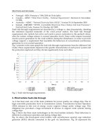
Fig. 15. Spectrogram of the real power [MW] at a turbine (times the turbines in the farm, 27).
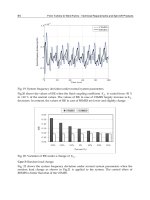
Active power in wind farm on a day

Fig. 16. Spectrogram of the real power [MW] at the substation.
0 5000 15000 25000 35000
From Turbine to Wind Farms - Technical Requirements and Spin-Off Products

126


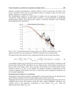
Fig. 17. Squared relative admittance
J
2
(f)/N
2
of the real power of the wind farm relative to
the turbine computed as the spectrogram ratio.


Fig. 18. Coherence models estimated by WINDFREDOM software.
Power Fluctuations in a Wind Farm Compared to a Single Turbine

127
Apart from the Short FFT (SFFT), the Wigner-Ville distribution (WVD) and the S-method
(SM) have been tested to increase the frequency resolution of the spectrogram. However, the
SFFT method has been found the most reliable since the amplitudes of the fluctuations are
less distorted by the abundant cross-terms present in the power output (Boashash, 2003).
Fig. 15 and Fig. 16 show the spectrogram in the centre of the picture, codified by the scale
shown on the right. The plots shown in this subsection have been produced with
WINDFREDOM software, which is freely available (Mur-Amada, 2009). The regions with

light colours (gray shades in the printed book) indicate that the power has a low content of
fluctuations of frequencies corresponding to the vertical axis at the time corresponding to
the horizontal axis. The zones with darker colours indicate that fluctuations of the frequency
corresponding to the vertical axis have been noticeably observed at the time corresponding
to the horizontal axis. For convenience, the median, the quartiles and the 5% and 95%
quantiles of the wind speed are also shown in the bottom of the figures. The periodogram is
shown on the left and it is computed by averaging the spectrogram.
Both the spectrogram and the periodogram show the auto-spectral density times frequency
in Fig. 15 and Fig. 16, because the frequency scale is logarithmic (the derivative of the
frequency logarithm is 1/
f ). Therefore, the shadowed area of the periodogram or the
darkness of the spectrogram is proportional to the variance of the power at each frequency.
Comparing Fig. 15 and Fig. 16, the fluctuations of frequencies higher than 40 cycles/day are
relatively smaller in the wind farm than in the turbine. The amount of smoothing at
different frequencies is just the squared relative admittance
J
2
(f)/N
2
in Fig. 17. For
convenience,
J
2
(f) has been divided by the number of turbines because J
2
(f)/N
2
~1 for
correlated fluctuations and
J

2
(f)/N
2
~ 1/N for uncorrelated fluctuations, (N = 27 is the
number of turbines in the wind farm.
The wind farm admittance, corresponding to the periodogram and spectrogram of Fig. 16
divided by Fig. 15 is shown in Fig. 17. The magnitude scale is logarithmic in this plot to
remark that the admittance reasonably fits a broken line in a double logarithmic scale.
In this farm, variations quicker than one and three-quarter of a minute (fluctuations of
frequency larger than 800 cycles/day) can be considered uncorrelated and fluctuations
lasting more than 36 minutes (fluctuations of frequency smaller than 40 cycles/day) can be
considered fully correlated. In the intermediate frequency band, the admittance decays as a
first order filter, in agreement with the spatial smoothing model.
Fig. 17 shows that the turbine and the wind farm medians (red and blue thick lines in the
bottom plot) are similar because slow fluctuations affect both systems alike. The interquartil
range (red and blue shadowed areas) is a bit larger in the scaled turbine power with respect
to the wind farm. The range has the same magnitude order because the daily variance is
primarily due to the correlated fluctuations, since the frequency content of the variance is
concentrated in frequencies lower than 40 cycles/day (see grey shadowed area in the
periodograms on the left of Fig. 15 and Fig. 16).
In practice, the oscillations measured in the turbine are seen, to some extent, in the
substation with some delay or in advance. The coherence
#1,#2
γ

is a complex magnitude
with modulus between 0 and 1 and a phase, which represent the delay (positive angles) or
the advance (negative angles) of the oscillations of the substation with respect to the turbine.
Since the spectrum of a signal is complex, the argument of the coherence
()

rc
f
γ

is the
average phase difference of the fluctuations.
From Turbine to Wind Farms - Technical Requirements and Spin-Off Products

128
The coherence
()
rc
f
γ

in Fig. 18 indicates the correlation degree and the time pattern of the
fluctuations. The modulus is analogous to the correlation coefficient of the spectrum lines
from both locations. If the ratio among complex power spectrums is constant (both in
modulus and phase), then the coherence is the unity and its argument is the average phase
difference. If the complex ratio is random (in modulus or phase), then the coherence is null.
The uncertainty of the coherence can be decreased smoothing the plot in Fig. 18. The black
broken line is the asymptotic approximation proposed in this chapter and the dashed and
dotted lines correspond to other mathematical fits of the coherence.



Fig. 19. Time delay quantiles between the fluctuation delays estimated by WINDFREDOM
software.

Fig. 20. Estimated phase delay between the power oscillations at the turbine and at the wind
farm output. The median value for each frequency f is presented on the left and the phase
differences of the spectrograms in Fig. 15 and Fig. 16 are presented on the right. A phase
unwrapping algorithm has been used to reconstruct the phase from the SFFT.
Power Fluctuations in a Wind Farm Compared to a Single Turbine

129
The shadowed area in Fig. 19 indicates the 5%, 25%, 50%, 75% and 95% quantiles of the time
delay τ between the oscillations observed at the turbine and the farm output. Fig. 19 shows
that the time delay is less than half an hour (0.02 days) the 90% of the time. However, the
time delay experiences great variability due to the stochastic nature of turbulence.
Wind direction is not considered in this study because it was steady during the data
presented in the chapter. However, the wind direction and the position of the reference
turbine inside the farm affect the time delay τ between oscillations. If wind direction
changes, the phase difference, Δϕ = 2π
f τ, can change notably in the transition frequency
band, leading to very low coherences in that band. In such cases, data should be divided
into series with similar atmospheric properties.
At frequencies lower than 40 cycles/day, the time delays in Fig. 19 implies small phase
differences, Δϕ = 2π
f τ (colorized in light cyan in Fig. 20), and fluctuations sum almost fully
correlated. At frequencies higher than 800 cycles/day, the phase difference Δϕ = 2π
f τ
usually exceeds several times ±2π radians (colorized in dark blue or white in Fig. 20), and
fluctuations sum almost fully uncorrelated. It should be noticed that the phase difference Δϕ
exceeds several revolutions at frequencies higher than 3000 cycles/day and the estimated
time delay in Fig. 10 has larger uncertainty (Ghiglia & Pritt, 1998). Thus, the unwrapping
phase method could cause the time delay to be smaller at higher frequencies in Fig. 11.
This methodology has been used in (Mur-Amada & Bayod-Rujula, 2010) to compare the
wind variations at several weather stations (wind speed behaves more linearly than

generated power). The WINDFREDOM software is free and it can be downloaded from
www.windygrid.org.
7. Conclusions
This chapter presents some data examples to illustrate a stochastic model that can be used to
estimate the smoothing effect of the spatial diversity of the wind across a wind farm on the
total generated power. The models developed in this chapter are based in the personal
experience gained designing and installing multipurpose data loggers for wind turbines,
and wind farms, and analyzing their time series.
Due to turbulence, vibration and control issues, the power injected in the grid has a
stochastic nature. There are many specific characteristics that impact notably the power
fluctuations between the first tower frequency (usually some tenths of Hertzs) and the grid
frequency. The realistic reproduction of power fluctuations needs a comprehensive model of
each turbine, which is usually confidential and private. Thus, it is easier to measure the
fluctuations in a site and estimate the behaviour in other wind farms.
Variations during the continuous operation of turbines are experimentally characterized for
timescales in the range of minutes to fractions of seconds. A stochastic model is derived in
the frequency domain to link the overall behaviour of a large number of wind turbines from
the operation of a single turbine. Some experimental measurements in the joint time-
frequency domain are presented to test the mathematical model of the fluctuations.
The admittance of the wind farm is defined as the ratio of the oscillations from a wind farm
to the fluctuations from a single turbine, representative of the operation of the turbines in
the farm. The partial cancellation of power fluctuations in a wind farm are estimated from
the ratio of the farm fluctuation relative to the fluctuation of one representative turbine.
From Turbine to Wind Farms - Technical Requirements and Spin-Off Products

130
Provided the Gaussian approximation is accurate enough, the wind farm power variability
is fully characterized by its auto spectrum and many interesting properties can be estimated
applying the outstanding properties of Gaussian processes (the mean power fluctuation
shape during a period, the distribution of power variation in a time period, the most

extreme power variation expected during a short period, etc.).
8. References
Abdi A.; Hashemi, H. & Nader-Esfahani, S. (2000). “On the PDF of the Sum of Random
Vectors”, IEEE Trans. on Communications. Vol. 48, No.1, January 2000, pp 7-12.
Alouini, M S.; Abdi, A. & Kaveh, M. (2001). “Sum of Gamma Variates and Performance of
Wireless Communication Systems Over Nakagami-Fading Channels”, IEEE Trans.
On Vehicular Technology, Vol. 50, No. 6, (2001) pp. 1471-1480.
Amarís, H. & Usaola J. (1997). Evaluación en el dominio de la frecuencia de las fluctuaciones
de tensión producidas por los generadores eólicos. V Jornadas Hispano-Lusas de
Ingeniería Eléctrica. 1997.
Apt, J. (2007) “The spectrum of power from wind turbines”, Journal of Power Sources 169
(2007) 369–374
Y. Baghzouz, R. F. Burch et alter (2002) “Time-Varying Harmonics: Part II—Harmonic
Summation and Propagation”, IEEE Trans. On Power Systems, Vol. 17, No. 1
(January 2002), pp. 279-285.
Bianchi, F. D.; De Battista, H. & Mantz, R. J. (2006). “Wind Turbine Control Systems.
Principles, Modelling and Gain Scheduling Design”, Springer, 2006.
Bierbooms, W.A.A.M. (2009) “Constrained Stochastic Simulation Of Wind Gusts For Wind
Turbine Design”, DUWIND Delft University Wind Energy Research Institute,
March 2009.
Boashash, B. (2003). "Time Frequency, Signal Analysis and Processing. A comprehensive
Reference". Ed. Elsevier, 2003.
Cavers, J.K. (2003). “Mobile Channel Characteristics”, 2
nd
ed., Shady Island Press, 2003.
Cidrás, J.; Feijóo, A.E.; González C. C., (2002). “Synchronization of Asynchronous Wind
Turbines” IEEE Trans, on Energy Conv., Vol. 17, No 4 (Nov. 2002), pp. 1162-1169
Comech-Moreno, M.P. (2007). “Análisis y ensayo de sistemas eólicos ante huecos de
tension”, Ph.D. Thesis, Zaragoza University, October 2007 (in Spanish).
Cushman-Roisin, B. (2007). “Environmental Fluid Mechanics”, John Wiley & Sons, 2007.

Frandsen, S.; Jørgensen, H.E. & Sørensen, J.D. (2007) “Relevant criteria for testing the quality
of turbulence models”, 2007 European Wind Energy Conference and Exhibition,
Milan (IT), 7-10 May 2007. pp. 128-132.
Gardner, W. A. (1994) “Cyclostationarity in Communications and Signal Processing”, IEEE
press, 1994.
Gardnera, W. A.; Napolitano, A. & Paurac, L. (2006) “Cyclostationarity: Half a century of
research”, Signal Processing 86 (April 2006), pp. 639–697.
Ghiglia, D.C. & Pritt, M.D. (1998). “Two-Dimensional Phase Unwrapping: Theory,
Algorithms, and Software”, John Whiley & Sons, 1998.
Hall, P.; & Heyde. C. C. (1980). Martingale Limit Theory and Its Application. New York:
Academic Press (1980).
Kaimal, J.C. (1978). “Horizontal Velocity Spectra in an Unstable Surface Layer” Journal of
the Atmospheric Sciences, Vol. 35, Issue 1 (January 1978), pp. 18–24.
Power Fluctuations in a Wind Farm Compared to a Single Turbine

131
Karaki, S. H. ; Salim B. A. & Chedid R. B. (2002). “Probabilistic Model of a Two-Site Wind
Energy Conversion System”, IEEE Transactions On Energy Conversion, Vol. 17,
No. 4, December 2002.
Kundur, P. P.; Balu, N. J.; Lauby, M. G. (1994). “Power System Stability and Control”,
McGraw-Hill, 1994.
Li, P.; Banakar, H.; Keung, P. K.; Far H.G. & Ooi B.T. (2007). “Macromodel of Spatial
Smoothing in Wind Farms”, IEEE Trans, on Energy Conv., Vol. 22, No 1 (March.
2007), pp 119-128.
Martins, A.; Costa, P.C. & Carvalho, A. S. (2006). “Coherence And Wakes In Wind Models
For Electromechanical And Power Systems Standard Simulations”, European Wind
Energy Conferences (EWEC 2006), February (2006), Athens.
Mur-Amada, J. (2009) “Wind Power Variability in the Grid”, PhD. Thesis, Zaragoza
University, October 2009. Available at www.windygrid.org
Mur-Amada, J. & Comech-Moreno, M.P. (2006). "Reactive Power Injection Strategies for

Wind Energy Regarding its Statistical Nature", Sixth International Workshop on
Large-Scale Integration of Wind Power and Transmission Networks for Offshore
Wind Farm. Delft, October 2006.
Mur-Amada, J. & Bayod-Rújula, A.A. (2007). "Characterization of Spectral Density of Wind
Farm Power Output", 9th Conference on Electrical Power Quality and Utilisation
(EPQU'2007), Barcelona, October 2007.
Mur-Amada, J. & Bayod-Rújula, A.A. (2010). "Variability of Wind and Wind Power", Wind
Power, Intech, Croatia, 2010. Available at: www.sciyo.com.
Norgaard, P. & Holttinen, H. (2004). "A Multi-turbine Power Curve Approach", in Proc. 2004
Nordic Wind Power Conference (NWPC 2002), Gothenberg, March 2004.
Press, W. H.; Teukolsky, S. A.; Vetterling, W. T. & Flannery, B. P. (2007). “Numerical Recipes.
The Art of Scientific Computing”, 3
rd
edition, Cambridge University Press, 2007.
Sanz M.; Llombart A.; Bayod A. A. & Mur, J. (2000) "Power quality measurements and
analysis for wind turbines", IEEE Instrumentation and Measurement Technical
Conference 2000, pp. 1167-1172. May 2000, Baltimore.
Saranyasoontorn, K.; Manuel, L. & Veers, P. S. “A Comparison of Standard Coherence
Models form Inflow Turbulence With Estimates from Field Measurements”, Journal
of Solar Energy Engineering, Vol. 126 (2004), Issue 4, pp. 1069-1082
Schlez, W. & Infield, D. (1998). “Horizontal, two point coherence for separations greater
than the measurement height”, Boundary-Layer Meteorology 87 (1998), 459-480.
Schwab, M.; Noll, P. & Sikora, T. (2006). “Noise robust relative transfer function estimation”,
XIV European Signal Processing Conference, September 4 - 8, 2006, Florence, Italy.
Soens, J. (2005). “Impact Of Wind Energy In A Future Power Grid”, Ph.D. Dissertation,
Katholieke Universiteit Leuven, December 2005.
Sorensen, P.; Hansen, A. D. & Rosas C. (2002). “Wind models for simulation of power
fluctuations from wind farms”, Journal of Wind Engineering and Ind.
Aerodynamics 90 (2002), pp. 1381-1402
Sørensen, P.; Cutululis, N. A.; Vigueras-Rodríguez, A; Madsen, H.; Pinson, P; Jensen, L. E.;

Hjerrild, J. & Donovan M., (2008) “Modelling of Power Fluctuations from Large
Offshore Wind Farms”, Wind Energy,Volume 11, Issue 1, pages 29–43,
January/February 2008.
From Turbine to Wind Farms - Technical Requirements and Spin-Off Products

132
Stefopoulos, G.; Meliopoulos A. P.& Cokkinides G. J. (2005), “Advanced Probabilistic Power
Flow Methodology”, 15th PSCC, Liege, 22-26 August 2005
Su, C-L. (2005) “Probabilistic Load-Flow Computation Using Point Estimate Method”, IEEE
Trans. Power Systems, Vol. 20, No. 4, November 2005, pp. 1843-1851.
Tentzerakis, S. T. & Papathanassiou S. A. (2007), “An Investigation of the Harmonic Emissions
of Wind Turbines”, IEEE Trans, on Energy Conv., Vol. 22, No 1, March. 2007, pp 150-
158.
Thiringer, T.; Petru, T.; & Lundberg, S. (2004) “Flicker Contribution From Wind Turbine
Installations” IEEE Trans, on Energy Conv., Vol. 19, No 1, March 2004, pp 157-163.
Vilar Moreno, C. (2003). “Voltage fluctuation due to constant speed wind generators” Ph.D.
Thesis, Carlos III University, Leganés, Spain, 2003.
Wangdee, W. & Billinton R. (2006). “Considering Load-Carrying Capability and Wind Speed
Correlation of WECS in Generation Adequacy Assessment”, IEEE Trans, on Energy
Conv., Vol. 21, No 3, September 2006, pp. 734-741.
Welfonder, E.; Neifer R. & Spaimer, M. (1997) “Development And Experimental
Identification Of Dynamic Models For Wind Turbines”, Control Eng. Practice, Vol.
5, No. 1 (January 2007), pp. 63-73.

Part 4
Input into Power System Networks

7
Distance Protections in the Power System Lines
with Connected Wind Farms

Adrian Halinka and Michał Szewczyk
Silesian University of Technology
Poland
1. Introduction
In recent years there has been an intensive effort to increase the participation of renewable
sources of electricity in the fuel and energy balance of many countries. In particular, this
relates to the power of wind farms (WF) attached to the power system at both the
distribution network (the level of MV and 110 kV) and the HV transmission network (220
kV and 400 kV)
1
. The number and the level of power (from a dozen to about 100 MW) of
wind farms attached to the power system are growing steadily, increasing the participation
and the role of such sources in the overall energy balance. Incorporating renewable energy
sources into the power system entails a number of new challenges for the power system
protections in that it will have an impact on distance protections which use the impedance
criteria as the basis for decision-making. The prevalence of distance protections in the
distribution networks of 110 kV and transmission networks necessitates an analysis of their
functioning in the new conditions. This study will be considering selected factors which
influence the proper functioning of distance protections in the distribution networks with
the wind farms connected to the power system.
2. Interaction of dispersed power generation sources (DPGS) with the power
grid
There are two main elements determining the character of work of the so-called dispersed
generation objects with the power grid. They are the type of the generator and the way of
connection.
In the case of using asynchronous generators, only parallel “cooperation” with the power
system is possible. This is due to the fact that reactive power is taken from the system for
magnetization. When the synchronous generator is used or the generator is connected by
the power converter, both parallel or autonomous (in the power island) work is possible.
The level of generating power and the quality of energy have to be taken into consideration

when dispersed power sources are to be connected to the distribution network. In regard to
wind farms, it should be emphasized that they are mainly connected to the HV distribution

1
The way of connection and power grid configuration differs in many countries. Sample configurations
are taken from the Polish Power Grid but can be easily adapted to the specific conditions in the
particular countries.
From Turbine to Wind Farms - Technical Requirements and Spin-Off Products

136
network for the reason of their relatively high generating power and not the best quality of
energy. This connection is usually made by the HV to MV transformer. It couples an internal
wind farm electrical network (on the MV level) with the HV distribution network. The
internal wind farm network consists of cable MV lines working in the trunk configuration
connecting individual wind turbines with the coupling HV/MV transformer. Fig. 1 shows a
sample structure of the internal wind farm network.

G6
TB6
G5
TB5
G4 T B4
G3 TB3
G2
TB2
0,4 km
1,0 km
0,4 km0,4 km
2,8 km
G12

TB12
G11 TB11
G10 TB10
G9 TB9
G8 TB8
G7
TB7
0,4 km0,6 km0,4 km
2,2 km
G18
TB18
G16 TB16
G17
TB17
G15 TB15
G14
TB14
G13
TB13
0,8 km
0,2 km
G24
TB24
G23 TB23
G22 TB22
G21
TB21
G20
TB20
G1 9

TB19
G30
TB30
G29 TB29
G27
TB27
G26
TB26
G25
TB25
G28
TB28
0,6 km
MV
HV
C
T1
G1
TB1
0,4 km
0,4 km
0,4 km
1,2 km1,0 km
0,4 km0,4 km
0,4 km1,0 km0,4 km
0,4 km
0,4 km
0,3 km
0,4 km1,2 km0,4 km0,4 km
0,6 km

TB36
G35
TB35
G34
TB34
G33
TB33
G32
TB32
G31
TB31
1,0 km
0,4 km0,4 km0,9 km0,4 km
2,8 km
HV
System A
HV
System B
B
L1
L2 L3 L4
D
A
E
Wind Far m
T2
WF Station
WFL
G36

Fig. 1. Sample structure of internal electrical network of the 72 MW wind farm connected to
the HV distribution network
There are different ways of connecting wind farms to the HV network depending, among
other things, on the power level of a wind farm, distance to the HV substation and the
number of wind farms connected to the sequencing lines. One can distinguish the following
characteristic types of connections of wind farms to the transmission network:
• Connection in the three-terminal scheme (Fig. 2a). For this form of connection the
lowest investment costs can be achieved. On the other hand, this form of connection
causes several serious technical problems, especially for the power system automation.
They are related to the proper faults detection and faults elimination in the
surroundings of the wind farm connection point. Currently, this is not the preferred
and recommended type of connection. Usually, the electrical power of such a wind
farm does not exceed a dozen or so MW.
• Connection to the HV busbars of the existing substation in the series of lines (Fig. 2b).
This is the most popular solution. The level of connected wind farms is typically in the
range of 5 to 80 MW.
• Connection by the cut of the line (Fig. 3.). This entails building a new substation. If the
farm is connected in the vicinity of an existing line, a separate wind farm feeder line is
superfluous. Only cut ends of the line have to be guided to the new wind farm power
substation. This substation can be made in the H configuration or the more complex 2
Distance Protections in the Power System Lines with Connected Wind Farms

137
circuit-breaker (2CB) configuration (Fig. 3b). The topology of the substation depends on
the number of the target wind farms connected to such a substation.

Substation A
HV
Substation B
HV

WF
HV
G1
TB 1
G2 TB2
G3
TB 3
WF
HV
G1
TB1
G2
TB2
G3
TB3
MV
MV
MV
a)
b)
Substation A
HV
Substation B
HV

Fig. 2. Types of the wind farm connection to HV network: a) three terminal-line , b)
connection to the busbars of existing HV/MV substation

Substation A
HV

Substation B
HV
WF1
1
HV
G1
TB1
G2
TB2
G3
TB3
WF 2
G1
TB 1
G2 TB2
G3 T B3
WF 1
HV
G1
TB1
G2
TB2
G3 T B3
WF 2
G1
TB1
G2
TB 2
G3
TB3

MV
MV
MV
HV
MV
HV
a) b)
Substation A
HV
Substation B
HV

Fig. 3. Connection of the wind farm to the HV network by the cutting of line: a) substation in
the H4 configuration, b) two-system 2CB configuration
• Connection to the HV switchgear of the EHV/HV substation bound to the transmission
network. In this case one of the existing HV line bays (Fig. 4a) or the separate
transformer (Fig. 4b) can be used. This form of connection is possible for wind farms of
high level generating powers (exceeding 100 MW). The influence of such a connection
on the proper functioning of the power protections is the lowest one.
From Turbine to Wind Farms - Technical Requirements and Spin-Off Products

138
HV
WF 2
G1
TB1
G2
TB2
G3
TB3

WF 1
G1
TB1
G2 TB2
G3
TB3
EHV
HV
WF 2
G1
TB1
G2
TB2
G3
TB3
WF 1
G1
TB1
G2 TB2
G3 TB3
EHV
HV
MV MV MV MV
a) b)

Fig. 4. Wind farm connection to the power system: a) by the existing switching bay of the
EHV/HV substation, b) by the HV busbars of the separate EHV/HV transformer
• Connection of the wind farm by the high voltage AC/DC link (Fig. 5). This form is most
commonly used for wind farms located on the sea and for different reasons cannot
work synchronously with the electrical power system. Using a direct current link is

useful for the control of operating conditions of the wind farm, however at the price of
higher investments costs.

System A
HV
WF
HV
G1
TB1
G2
TB2
G3 TB3
MV
MV
DC
AC/DC
DC/AC
HV
~
~
System B
HV

Fig. 5. Connection of the wind farm by the AC/DC link
Due to the limited number of system EHV/HV substations and the relatively high distances
between substations and wind farms, most of them are connected to the existing or newly
built HV/MV substations inside the HV line series.