From Turbine to Wind Farms Technical Requirements and Spin-Off Products Part 11 pdf

Distance Protections in the Power System Lines with Connected Wind Farms

139
3. Technical requirements for the dispersed power sources connected to the
distribution network
Basic requirements for dispersed power sources are stipulated by a number of directives
and instructions provided by the power system network operator. They contain a wide
spectrum of technical conditions which must be met when such objects are connected to the
distribution network. From the point of view of the power system automation, these
requirements are mainly concerned with the possibilities of the power level and voltage
regulation. Additionally, the behaviour of a wind farm during faults in the network and the
functioning of power protection automation have to be determined. Wind farms connected
to the HV distribution network should be equipped with the remote control, regulation and
monitoring systems which enable following operation modes:
• operation without limitations (depending on the weather conditions),
• operation with an assumed a priori power factor and limited power generation,
• intervention operation during emergences and faults in the power system (type of
intervention is defined by the operator of the distribution network),
• voltage regulator at the connection point,
• participation in the frequency regulation (this type of work is suitable for wind farms of
the generating power greater than 50 MW).
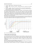
During faults in HV network, when significant changes (dips) of voltage occur, wind farm
cannot loose the capability for reactive power regulation and should actively work towards
sustaining the voltage level in the network. It also should maintain continuous operation in
the case of faults in the distribution network which cause voltage dips at the wind farm
connection point, of the times over the borderline shown in Fig. 6.


Fig. 6. Borderline of voltage level conditioning continuous wind farm operation during
faults in the distribution network
4. Dispersed power generation sources in fault conditions

The behaviour of a power system in dynamic fault states is much more complicated for the
reason of the presence of dispersed power sources than when only the conventional ones are
in existence. This is a direct consequence of such factors as the technical construction of
driving units, different types of generators, the method of connection to the distribution
From Turbine to Wind Farms - Technical Requirements and Spin-Off Products

140
network, regulators and control units, the presence of fault ride-through function as well as
a wide range of the generating power determined by e.g. the weather conditions.
Taking the level of fault current as the division criteria, the following classification of
dispersed power sources can be suggested:
• sources generating a constant fault current on a much higher level than the nominal
current (mainly sources with synchronous generators),
• sources generating a constant fault current close to the nominal current (units with
DFIG generators or units connected by the power converters with the fault ride-through
function),
• sources not designed for operation in faulty conditions (sources with asynchronous
generators or units with power converters without the fault ride-through function).
Sources with synchronous generators are capable of generating a constant fault current of
higher level than the nominal one. This ability is connected with the excitation unit
which is employed and with the voltage regulator. Synchronous generators with an
electromechanical excitation unit are capable of holding up a three-phase fault current of the
level of three times or higher than the nominal current for a few seconds. For the electronic
(static) excitation units, in the case of a close three-phase fault, it is dropping to zero after the
disappearance of transients. This is due to the little value of voltage on the output of the
generator during a close three-phase fault.
For asynchronous generators, the course of a three-phase current on its outputs is only
limited by the fault impedance. The fault current drops to zero in about (0,2 ÷ 0,3) s. The
maximum impulse current is close to the inrush current during the motor start-up of the
generator (Lubośny, 2003). The value of such a current for typical machines is five times

higher than the nominal current. This property makes it possible to limit the influence of
such sources only on the initial value of the fault current and value of the impulse current.
The construction and parameters of the power converters in the power output circuit
determine the level of fault current for such dispersed power sources. Depending on the
construction, they generate a constant fault current on the level of its nominal current or are
immediately cut off from the distribution network after a detection of a fault. If the latter is
the case, only a current impulse is generated just after the beginning of a fault.
A common characteristic of dispersed sources cooperating with the power system is the fact
that they can achieve local stability. Some of the construction features (power converters)
and regulatory capabilities (reactive power, frequency regulation) make the dispersed
power generation sources units highly capable of maintaining the stability in the local
network area during the faulty conditions (Lubośny, 2003).
Dynamic states analyses must take into consideration the fact that present wind turbines are
characterized by much higher resistance to faults (voltage dips) to be found in the power
system than the conventional power sources based on the synchronous generators. A very
important and useful feature of some wind turbines equipped with power converters, is the
fact that they can operate in a higher frequency range (43 ÷ 57 Hz) than in conventional
sources (47 ÷ 53 Hz) (Ungrad et al., 1995).
Dispersed generation may have a positive influence on the stability of the local network
structures: dispersed source – distribution network during the faults. Whether or not it can be
well exploited, depends on the proper functioning of the power system protection
automation dedicated to the distribution network and dispersed power generation
sources.
Distance Protections in the Power System Lines with Connected Wind Farms

141
5. Influence of connecting dispersed power generating sources to the
distribution network on the proper functioning of power system protections
In the Polish power system most of generating power plants (the so-called system power
plants) are connected to the HV and EHV (220 kV and 400 kV) transmission networks. Next,

HV networks are usually treated as distribution networks powered by the HV transmission
networks. This results in the lack of adaptation of the power system protection automation
in the distribution network to the presence of power generating sources on those (MV and
HV) voltage levels.
Even more frequently, using of the DPGS, mainly wind farms, is the source of potential
problems with the proper functioning of power protection automation. The basic functions
vulnerable to the improper functioning in such conditions are:
• primary protection functions of lines,
• earth-fault protection functions of lines,
• restitution automation, especially auto-reclosing function,
• overload functions of lines due the application of high temperature low sag conductors
and the thermal line rating,
• functions controlling an undesirable transition to the power island with the local power
generation sources.
The subsequent part of this paper will focus only on the influence of the presence of the
wind farms on the correctness of action of impedance criteria in distance protections.
5.1 Selected aspects of an incorrect action of the distance protections in HV lines
Distance protection provides short-circuit protection of universal application. It constitutes a
basis for network protection in transmission systems and meshed distribution systems. Its
mode of operation is based upon the measurement and evaluation of the short-circuit
impedance, which in the typical case is proportional to the distance to the fault. They rarely
use pilot lines in the 110 kV distribution network for exchange of data between the endings
of lines. For the primary protection function, comparative criteria are also used. They take
advantage of currents and/or phases comparisons and use of pilot communication lines.
However, they are usually used in the short-length lines (Ungrad et al., 1995).
The presence of the DPGS (wind farms) in the HV distribution network will affect the
impedance criteria especially due to the factors listed below:
• highly changeable value of the fault current from a wind farm. For wind farms
equipped with power converters, taking its reaction time for a fault, the fault current is
limited by them to the value close to the nominal current after typically not more then

50 ms. So the impact of that component on the total fault current evaluated in the
location of protection is relatively low.
• intermediate in-feed effect at the wind farm connection point. For protection realizing
distance principles on a series of lines, this causes an incorrect fault localization both in
the primary and the back-up zones,
• high dynamic changes of the wind farm generating power. Those influence the more
frequent and significant fluctuations of the power flow in the distribution network.
They are not only limited to the value of the load currents but also to changes of their
directions. In many cases a load of high values must be transmitted. Thus, it is
necessary to use wires of higher diameter or to apply high temperature low sag
From Turbine to Wind Farms - Technical Requirements and Spin-Off Products

142
conductors or thermal line rating schemes (dynamically adjusting the maximum load to
the seasons or the existing weather conditions). Operating and load area characteristics
may overlap in these cases.
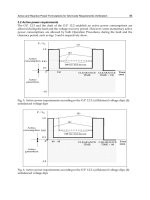
Setting distance protections for power lines
In the case of distance protections, a three-grading plan (Fig. 7) is frequently used.
Additionally, there are also start-up characteristic and the optional reverse zone which reach
the busbars.


Substation 2
System
B
System
A
DB C A
ABA
ZZ 9.0

1
=
(
)
BCABA
ZZZ 9.09.0
2
+
=
(
)
[
]
CDBCABA
ZZZZ 9.09.09.0
3
+
+
=
st 0
1
≅
stt
Δ
=
2
stt
Δ
=
2

3
Substation 1
t
w
[s]
E

Fig. 7. Three-grading plan of distance protection on series of lines
The following principles can be used when the digital protection terminal is located in the
substation A (Fig. 7) (Ziegler, 1999):
• impedance reach of the first zone is set to 90 % of the A-B line-length

1
0.9
A
A
B
ZZ= (1)
tripping time t
1
=0 s;
•
impedance reach of the second zone cannot exceed the impedance reach of the first
zone of protection located in the substation B

(
)
2
0.9 0.9
A

AB BC
ZZZ=+ (2)
tripping time should be one step higher than the first one t
2
=Δt s from the range of
(0.3÷0.5) s. Typically for the digital protections and fast switches, a delay of 0.3 s is
taken;
•
impedance reach of the third zone is maximum 90% of the second zone of the shortest
line outgoing from the subsubstation B:

()
3
0.9 0.9 0.9
A
AB BC CD
ZZZZ
⎡
⎤
=++
⎣
⎦
(3)
For the selectivity condition, tripping time for this zone cannot by shorter than t
3
=2Δt s.
Improper fault elimination due to the low fault current value

As mentioned before, when the fault current flowing from the DPGS is close to the nominal
current, in most of cases overcurrent and distance criteria are difficult or even impossible to

apply for the proper fault elimination (Pradhan & Geza, 2007). Figure 8 presents sample
Distance Protections in the Power System Lines with Connected Wind Farms

143
courses of the rms value of voltage U, current I, active and reactive power (P and Q) when
there are voltage dips caused by faults in the network. The recordings are from a wind
turbine equipped with a 2 MW generator with a fault ride-through function (Datasheet,
Vestas). This function permits wind farm operation during voltage dips, which is generally
required for wind farms connected to the HV networks.


Fig. 8. Courses of electric quantities for Vestas V80 wind turbine of 2 MW: a) voltage dip to
0.6 U
N
, b) voltage dip to 0.15 U
N
(Datasheet, Vestas)
Analyzing the course of the current presented in Fig. 8, it can be observed that it is close to
the nominal value and in fact independent a of voltage dip. Basing on the technical data it is
possible to approximate t
1
time, when the steady-state current will be close to the nominal
value (Fig. 9).


Fig. 9. Linear approximation of current and voltage values for the wind turbine with DFIG
generator during voltage dips: U
G
– voltage on generator outputs, I
G

– current on generator
outputs, I
Im_G
– generator reactive current, t
1
≈50 ms, t
3
-t
2
≈100 ms
From Turbine to Wind Farms - Technical Requirements and Spin-Off Products

144
0,1
0,2 0,3
0,4
0,5
0,6
0,7 0,8 0,9
1,0
1,0
I
Im_g
[p.u.]
U
G
[p.u.]
0,1
0,2
0,3

0,4
0,5
0,6
0,7
0,8
0,9
0,0
0,0
stator connected in delta
stator connected in star
3
2,0
3
1

Fig. 10. Course of the wind turbine reactive current
The negative influence of the low value steady current from the wind farm is cumulating
especially when the distribution network is operating in the open configuration (Fig. 11).

HV
C
T1
System A
System B
B
L1 L2 L3
L4
D
A
E

T2
WF
F
LWF
HV
MV
HV
Swiched-off
line

Fig. 11. Wind farm in the distribution network operating in the open configuration
The selected wind turbine is the one most frequently used in the Polish power grid. The
impulse current at the beginning of the fault is reduced to the value of the nominal current
after 50 ms. Additionally, the current has the capacitance character and is only dependent
on the stator star/delta connection. This current has the nominal value for delta connection
(high rotation speed of turbine) and nominal value divided by
3 for the star connection as
presented in Fig. 9.
Distance Protections in the Power System Lines with Connected Wind Farms

145
Reaction of protection automation systems in this configuration can be estimated comparing
the fault current to the pick-up currents of protections. For a three-phase fault at point F
(Fig. 11) the steady fault current flowing through the wind farm cannot exceed the nominal
current of the line. The steady fault current of the single wind turbine of P
N
=2 MW (S
N
=2.04
MW) is I

k
= I
NG
= 10.7 A at the HV side (delta stator connection). However initial fault
current
"
k
I is 3,3 times higher than the nominal current (
"
35.31 A
k
I = ).It must be emphasized
that the number of working wind turbines at the moment of a fault is not predictable. This
of course depends on weather conditions or the network operator’s requirements. All these
influence a variable fault current flowing from a wind farm. In many cases there is a starting
function of the distance protection in the form of a start-up current at the level of 20% of the
nominal current of the protected line. Taking 600 A as the typical line nominal current, even
several wind turbines working simultaneously are not able to exceed the pick-up value both
in the initial and the steady state fault conditions. When the impedance function is used for
the pick-up of the distance protection, the occurrence of high inaccuracy and fluctuations of
measuring impedance parameters are expected, especially in the transient states from the
initial to steady fault conditions.
The following considerations will present a potential vulnerability of the power system
distribution networks to the improper (missing) operation of power line protections with
connected wind farms. In such situations, when there is a low fault current flow from a
wind farm, even using the alternative comparison criteria will not result in the improvement
of its operation. It is because of the pick-up value which is generally set at (1,2 ÷ 1,5) I
N
.
To minimize the negative consequences of functioning of power system protection

automation in HV network operating in an open configuration with connected wind farms,
the following instructions should be taken:
•
limiting the generated power and/or turning off the wind farm in the case of a radial
connection of the wind farm with the power system. In this case, as a result of planned
or fault switch-offs, low fault WF current occurs,
•
applying distance protection terminals equipped with the weak end infeed logic on all
of the series of HV lines, on which the wind farm is connected. The consequences are
building up the fast teletransmission network and relatively high investment costs,
•
using banks of settings, configuring adaptive distance protection for variant operation
of the network structure causing different fault current flows. When the HV
distribution network is operating in a close configuration, the fault currents
considerably exceed the nominal currents of power network elements. In the radial
configuration, the fault current which flows from the local power source will be under
the nominal value.
Selected factors influencing improper fault location of the distance protections of lines

In the case of modifying the network structure by inserting additional power sources, i.e.
wind farms, the intermediate in-feeds occur. This effect is the source of impedance paths
measurement errors, especially when a wind farm is connected in a three-terminal
configuration. Figure 12a shows the network structure and Fig. 12b a short-circuit
equivalent scheme for three-phase faults on the M-F segment. Without considering the
measuring transformers, voltage U
p
in the station A is:

(
)

AM A MF Z AM A MF A WF
p
UZIZIZIZII=+=+ + (4)
From Turbine to Wind Farms - Technical Requirements and Spin-Off Products

146
On the other hand current I
p
measured by the protection in the initial time of fault is the
fault current I
A
flowing in the segment A-M. Thus the evaluated impedance is:

(
)
1
p
AM A MF A WF
WF
pAMMFAMMF
i
f
pA A
U
ZI Z I I
I
ZZZZZk
II I
++
⎛⎞

== = + + = +
⎜⎟
⎝⎠
(5)
where:
U
p
– positive sequence voltage component on the primary side of voltage transformers at
point A,
I
p
– positive sequence current component on the primary side of current transformers at
point A,
I
A
– fault current flowing from system A,
I
WF
– fault current flowing from WF,
Z
AM


– impedance of the AM segment,
Z
MF
– impedance of the MF segment,
k
if
– intermediate in-feed factor.

W
2
W
1
WF
W
3
I
A
F
M
A
System
I
A
+I
WF
I
WF
a)
E
SA
E
SB
E
WF
A
MBF
WF

Z
SA
Z
AM
Z
MF
Z
FB
Z
SE
I
A
I
A
+I
WF
I
WF
Z
WF M
Z
WF
b)
B
System

Fig. 12. Teed feeders configuration a) general scheme, b) equivalent short-circuit scheme.
It is evident that estimated from (5) impedance is influenced by error ΔZ:

WF

MF
A
I
ZZ
I
Δ= (6)
The error level is dependent on the quotient of fault current
Z
I from system A and power
source WF (wind farm). Next the error is always positive so the impedance reaches of the
operating characteristics are shorter. Evaluating the error level from the impedance of the
equivalent short-circuit:

SA AM
MF
WF WFM
ZZ
ZZ
ZZ
+
Δ=
+
(7)
Equation (7) shows the significant impact on the error level of short-circuit powers
(impedances of power sources), location of faults (
,
AM FWM
ZZ
) and types of faults.
Minimizing possible errors in the evaluation of impedance can be achieved by modifying

the reaches of operating characteristics covering the WF location point. Thus the reaches of
the second and the third zone of protection located at point A (Fig. 7) are:
Distance Protections in the Power System Lines with Connected Wind Farms

147

()
2
0.9 0.9 0.9 0.9 1
WF
A
AB BC AB BC
if
A
I
ZZZk ZZ
I
⎡
⎤
⎛⎞
=+ =+ +
⎢
⎥
⎜⎟
⎢
⎥
⎝⎠
⎣
⎦
(8)

() ()
3
0.9 0.9 0.9 0.9 0.9 0.9 1
WF
A ABBCCD ABBCCD
if
A
I
ZZZZk ZZZ
I
⎡
⎤
⎛⎞
⎡⎤
=++ =++ +
⎢
⎥
⎜⎟
⎣⎦
⎢
⎥
⎝⎠
⎣
⎦
(9)
It is also necessary to modify of the first zone, i.e.:

1
0.9 0.9 1

WF
A
AB AB
if
A
I
ZZkZ
I
⎛⎞
==+
⎜⎟
⎝⎠
(10)
This error correction is successful if the error level described by equations (6) and (7) is
constant. But for wind farms this is a functional relation. The arguments of the function are,
among others, the impedance of WF Z
WF
and a fault current I
WF
. These parameters are
dependent on the number of operating wind turbines, distance from the ends of the line to
the WF connection point (point M in Fig. 12a), fault location and the time elapsed from the
beginning of a fault (including initial or steady fault current of WF).
As mentioned before, the three-terminal line connection of the WF in faulty conditions
causes shortening of reaches of all operating impedance characteristics in the direction to the
line. This concerns both protections located in substation A and WF. For the reason of
reaching reduction level, it can lead to:
•
extended time of fault elimination, e.g. fault elimination will be done with the time of
the second zone instead of the first one,

•
improper fault elimination during the auto-reclosure cycles. This can occurs when
during the intermediate in-feed the reaches of the first extended zones overcome
shortening and will not reach full length of the line. Then what cannot be reached is
simultaneously cutting-off the fault current and the pick-up of auto-reclosure
automation on all the line ends.
In Polish HV distribution networks the back-up protection is usually realized by the second
and third zones of distance protections located on the adjacent lines. With the presence of
the WF (Fig. 13), this back-up protection can be ineffective.
As an example, in connecting WF to substation C operating in a series of lines A-E what
should be expected is the miscalculation of impedances in the case of intermediate in-feed in
substation C from the direction of WF. The protection of line L2 located in substation B,
when the fault occurs at point F on the line L3, “sees” the impedance vector in its second or
third zone. The error can be obtained from the equation:

(
)
22
2
LBC L WF
pB
CF
p
BBCCF
p
B
pB L
IZ I I Z
U
ZZZZ

II
++
== =++Δ (11)
where:
U
pB
– positive sequence voltage on the primary side of voltage transformers at point B,
I
pB
– positive sequence current on the primary side of current transformers at point B,
I
L2
– fault current flowing by the line L2 from system A,
I
WF
– fault current from WF,
From Turbine to Wind Farms - Technical Requirements and Spin-Off Products

148
Z
BC
– line L2 impedance,
Z
CF
– impedance of segment CF of the line L3
and the error ΔZ
pB
is defined as:

2

WF
pB CF
L
I
ZZ
I
⎛⎞
Δ=
⎜⎟
⎝⎠
. (12)

E
SA
E
SB
E
WF
A
BC DEF
WF
Z
SA
Z
AB
Z
BC
Z
CF
Z

FD
Z
DE
Z
SE
I
AB
I
AB
+I
WF
I
WF
C
T1
HV
System A
HV
System B
B
L1
L2
L3 L4
D
A
E
T2
WF
F
LW

F
I
L2
I
F
W
I
L2
+I
WF
SN
HV
a)
b)
Z
WFC
Z
WF

Fig. 13. Currents flow after the WF connection to substation C: a) general scheme, b)
simplified equivalent short-circuit scheme
It must be emphasized that, as before, also the impedance reaches of second and third zones
of LWF protection located in substation WF are reduced due to the intermediate in-feed.
Due to the importance of the back-up protection, it is essential to do the verification of the
proper functioning (including the selectivity) of the second and third zones of adjacent lines
with wind farm connected. However, due to the functional dynamic relations, which cause
the miscalculations of the impedance components, preserving the proper functioning of the
distance criteria is hard and requires strong teleinformatic structure and adaptive decision-
making systems (Halinka et al., 2006).
Overlapping of the operating and admitted load characteristics

The number of connected wind farms has triggered an increase of power transferred by the
HV lines. As far as the functioning of distance protection is concerned, this leads to the
increase of the admitted load of HV lines and brings closer the operating and admitted load
characteristics. In the case of non-modified settings of distance protections this can lead to
the overlapping of these characteristics (Fig 14).
Distance Protections in the Power System Lines with Connected Wind Farms

149
The situation when such characteristics have any common points is unacceptable. This
results in unneeded cuts-off during the normal operation of distribution network. Unneeded
cuts-off of highly loaded lines lead to increases of loads of adjacent lines and cascading
failures potentially culminating in blackouts.

R
p
jX
p
Operating characteristic
'
Admitted load
characteristic
.
8.0cos
capload
=ϕ
.
8.0cos
indload
=ϕ

1cos =
load
ϕ
minp
Z

Fig. 14. Overlapping of operating and admitted load characteristics
The impedance area covering the admitted loads of a power line is dependent on the level
and the character of load. This means that the variable parameters are both the amplitude
and the phase part of the impedance vector. In normal operating conditions the amplitude
of load impedance changes from Z
pmin
practically to the infinity (unloaded line). The phase
of load usually changes from cosφ = 0.8
ind
to cosφ = 0.8
cap
. The expected Z
pmin
can be
determined by the following equation (Ungrad et al., 1995), (Schau et al., 2008):

2
min min
min
max
max
3
pp
p

p
p
UU
Z
S
I
==
⋅
, (13)
where:
U
pmin
– minimal admitted operating voltage in kV (usually U
pmin
= 0,9 U
N
),
S
pmax
– maximum apparent power in MVA,
I
pmax
– maximum admitted load.
A necessary condition of connecting DPGS to the HV network is researching whether the
increase of load (especially in faulty conditions e.g. one of the lines is falling out) is not
leading to an overlap. Because of the security reasons and the falsifying factors influencing
the impedance evaluation, it is assumed that the protection will not unnecessarily pick-up if
the impedance reach of operating zones will be shorter than 80% of the minimal expected
load. This requirement will be practically impossible to meet especially when the MHO
starting characteristics are used (Fig 15a). There are more possibilities when the protection

realizes a distance protection function with polygonal characteristics (Fig. 15b).
Using digital distance protections with polygonal characteristics is also very effective for HV
lines equipped with high temperature low sag conductors or thermal line rating. In this case
From Turbine to Wind Farms - Technical Requirements and Spin-Off Products

150
the load can increase 2.5 times. Figure 16 shows the adaptation of an impedance area to the
maximum expected power line load. Of course this implies serious problems with the
recognition of faults with high resistances.


R
p
jX
p
Z
L
Z
r
Z
IV
Z
III
Z
II
Z
I
b)
Z
REV

jX
p
a )
R
p
Z
L
Z
I
Z
II
Z
III
Z
r


Fig. 15. Starting and operating characteristics a) MHO, b) polygonal


R
p
jX
p
Area of starting and operating characteristics
Load impedance area
Z
L
Z
r

Z
IV
Z
III
Z
II
Z
I
Z
REV
capLoad
8.0cos =ϕ
indLoad
8.0cos =ϕ
1cos =
Load
ϕ


Fig. 16. Adaptation of operating characteristics to the load impedance area
Distance Protections in the Power System Lines with Connected Wind Farms

151
5.2 Simulations
Figure 17 shows the network structure taken for the determination of the influence of
selected factors on the impedance evaluation error. This is a part of the 110 kV network of
the following parameters:
•
short-circuit powers of equivalent systems:
"

1000
kA
S = MVA,
"
500
kB
S = MVA;
•
wind farm consists of 30 wind turbines using double fed induction generators of the
individual power P
jN
=2 MW with a fault ride-through function. Power of a wind farm
is changing from 10% to 100% of the nominal power of the wind farm. WF is connected
in the three-terminal line scheme,
•
overhead power line AB:
•
length: 30 km; resistance per km: r
l
=0.12 Ω/km, reactance per km x
j
=0.4 Ω/km
•
overhead power output line from WF:
•
length: 2 km; resistance per km: r
l
=0.12 Ω/km, reactance per km x
j
=0.4 Ω/km

•
metallic three-phase fault on line AB between the M connection point and 100% of the
line L
A-B
length.
Initial and steady fault currents from the wind farm and system A have been evaluated for
these parameters. It has been assumed that phases of these currents are equal. The initial
fault current of individual wind turbines will be limited to 330% of the nominal current of
the generator and wind turbines will generate steady fault current on the level of 110% of
the nominal current of the generator. The following examples will now be considered.



20 kV
WF
110 kV
S
y
stem B
S
y
stem A
A
C
M
B
MVAS
kA
1000
"

=

MVAS
kB
500
"
=

(
)
NWFWF
PP %10010 ÷=

2km
30 km
F
F

Fig. 17. Network scheme for simulations

Example 1

The network is operating in quasi-steady conditions. The farm is generating power of 60
MW and is connected at 10 % of the L
A-B
line length. The location of a fault changeable from
20 % to 100 % of the L
A-B
length with steps of 10 %. Table 1 presents selected results of
simulations for faults of times not exceeding 50 ms. Results take into consideration the

limitation of fault currents on the level of 330% of the nominal current of the generator. By
analogy, Table 2 shows the results when the limitation is 110 % after a reaction of the control
units.
From Turbine to Wind Farms - Technical Requirements and Spin-Off Products

152
Fault location
l
x
%
Z
LAB
A
I

C
I

CA
II

ΔR ΔX
%R
δ

%X
δ

R
LAF

X
LAF
[km] [%] [kA] [kA] [-]
[Ω] [Ω]
[%] [%]
[Ω] [Ω]
6 20 3.93 0.801 0.204 0.073 0.245 10.191 10.191 0.720 2.400
9 30 3.591 0.732 0.204 0.147 0.489 13.590 13.590 1.080 3.600
12 40 3.305 0.674 0.204 0.220 0.734 15.295 15.295 1.440 4.800
15 50 3.061 0.624 0.204 0.294 0.979 16.308 16.308 1.800 6.000
18 60 2.851 0.581 0.204 0.367 1.223 16.982 16.982 2.160 7.200
21 70 2.667 0.545 0.204 0.441 1.471 17.516 17.516 2.520 8.400
24 80 2.505 0.511 0.204 0.514 1.714 17.849 17.849 2.880 9.600
27 90 2.362 0.481 0.204 0.586 1.955 18.101 18.101 3.240 10.800
30 100 2.234 0.455 0.204 0.660 2.200 18.330 18.330 3.600 12.000
Table 1. Initial fault currents and impedance errors for protection located in station A
depending on the distance to the location of a fault (Case 1)
where:
l – distance to a fault from station A,
x
%
Z
LAB
– distance to a fault in the percentage of the L
AB
length,
A
I – rms value of the initial fault current flowing from system A to the point of fault,
C
I – rms value of the initial current flowing from WF to the point of a fault,

ΔR – absolute error of the resistance evaluation of the impedance algorithm,
(
)
{
}
Re
CA
LMF
RIIZΔ= ,
ΔX – absolute error of the reactance evaluation of the impedance algorithm,
(
)
{
}
Im
CA
LMF
XIIZΔ= ,
R
LAF
– real value of the resistance of the fault loop,
X
LAF
– real value of the reactance of the fault loop,
%R
δ
– relative error of the evaluation of the resistance
%RLAF
RR
δ

=
Δ ,
%X
δ
– relative error of the evaluation of the resistance,
%XLAF
XX
δ
=Δ .

Fault location
l
x
%
Z
LAB
()
A
u
I
()Cu
I
() ()Cu Au
II
ΔR ΔX
%R
δ

%X
δ

[km] [%] [kA] [kA] [-]
[Ω] [Ω]
[%] [%]
6 20 3.986 0.328 0.082 0.030 0.099 4.114 4.114
9 30 3.685 0.328 0.089 0.064 0.214 5.934 5.934
12 40 3.425 0.328 0.096 0.103 0.345 7.182 7.182
15 50 3.199 0.328 0.103 0.148 0.492 8.203 8.203
18 60 3 0.328 0.109 0.197 0.656 9.111 9.111
21 70 2.824 0.328 0.116 0.251 0.836 9.955 9.955
24 80 2.666 0.328 0.123 0.310 1.033 10.765 10.765
27 90 2.525 0.328 0.130 0.374 1.247 11.547 11.547
30 100 2.398 0.328 0.137 0.443 1.477 12.310 12.310
Table 2. Steady fault currents and impedance errors for protection located in station A
depending on the distance to the location of a fault (Case 2)
Distance Protections in the Power System Lines with Connected Wind Farms

153
where:
()
A
u
I - rms value of steady fault current flowing from system A to the point of a fault,
()Cu
I - rms value of steady fault current flowing from WF to the point of a fault,
The above-mentioned tests confirm that the presence of sources of constant generated
power (WF) brings about the miscalculation of impedance components. The error is rising
with the distancing from busbars in substation A to the point of a fault, but does not exceed
20 %. It can be observed at the beginning of a fault that the error level is higher than in the
case of action of the wind farm control units. It is directly connected with the quotient of

currents from system A and WF. In the first case it is constant and equals 0.204. In the
second one it is lower but variable and it is rising with the distance from busbars of
substation A to the point of a fault.
From the point of view of distance protection located in station C powered by WF, the error
level of evaluated impedance parameters is much higher and exceeds 450 %. It is due to the
high
A
C
II ratio which is 4.9. Figure 18 shows a comparison of a relative error of estimated
reactance component of the impedance fault loop for protection located in substation A
(system A) and station C (WF).

0,000
50,000
100,000
150,000
200,000
250,000
300,000
350,000
400,000
450,000
500,000
6 9 12 15 18 21 24 27 30
l [km]
System A
WF
Relative error [%]

Fig. 18. Relative error (%) of reactance estimation in distance protection in substation A and
C in relation to the distance to a fault
Attempting to compare estimates of impedance components for distance protections in
substations A, B and C in relation to the distance to a fault, the following analysis has been
undertaken for the network structure as in Fig. 19. Again a three-terminal line of WF
connection has been chosen as the most problematic one for power system protections. For
this variant WF consists of 25 wind turbines equipped as before with DFIG generators each
of 2 MW power. The selection of such a type of generator is dictated by its high fault
currents when compared with generators with power converters in the power output path
and the popularity of the first ones.
Figure 20 shows the influence of the location of a fault on the divergence of impedance
components evaluation in substations A, B and C in comparison to the real expected values.
The presented values are for the initial time of a three-phase fault on line A-B with the
assumption that all wind turbines are operating simultaneously, generating the nominal
power.