From Turbine to Wind Farms Technical Requirements and Spin-Off Products Part 12 pptx

From Turbine to Wind Farms - Technical Requirements and Spin-Off Products

154

20 kV
WF
110 kV
System B
Syste
m
A
A
C
M
B
MVAS
kA
1000
"
=
MVAS
kB
500
"
=

6k
m
30 km
P
WF

=50 MW
10 km
110 kV

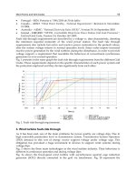
Fig. 19. Network scheme for the second stage of simulations

0

20

40 60 80 100
0

4

8

12

16

20

Amplitude of the impedance fault loop [Ω]

Line length [%]
Distance protection ZA


connection point

Real values
Evaluated values

0
20 40 60 80

100

0
4
8
12
16
20
Amplitude of the impedance [fault loop [Ω]

Line len
g
th [%]
Distance protection ZB




connection point

Real values

Evaluated values

0

20 40 60 80 100
0

10

20

30

40

50

Line length [%]
Distance protection ZC



connection point
Real values
Evaluated values
Amplitude of the impedance fault loop [Ω]

0
20 40 60 80

100

0
50
100
150
200
250
Relative error of the impedance
fault loop evaluation [%]

Line length [%]



connection point
ZA

ZB

ZC



Fig. 20. Divergences between the evaluated and expected values of the amplitude of
impedance for protections in substations A, B and C
Analyzing courses in Fig. 20, it can be observed that the highest inaccuracy in the amplitude
of impedance evaluation concerns protections in substation C. The divergences between
evaluated and expected values are rising along with the distance from the measuring point
to the location of fault. It is characteristic that in substations A and B these divergences are at
least one class lower than for substation C. This is the consequence of a significant

Distance Protections in the Power System Lines with Connected Wind Farms

155
disproportion of the short-circuit powers of systems A and B in relation to the nominal
power of WF.
On the other hand, for the fault in the C-M segment of line the evaluation error of an
impedance fault loop is rising for distance protections in substations A and B. For distance
protection in substation B a relative error is 53 % at fault point located 4 km from the
busbars of substation C. For distance of 2 km from station C the error exceeds 86 % of the
real impedance to the location of a fault (Lubośny, 2003).
Example 2

The network as in Figure 17 is operating with variable generating power of WF from 100 %
to 10 % of the nominal power. The connection point is at 10 % of the line L
A-B
length. A
simulated fault is located at 90 % of the L
A-B
length.
Table 3 shows the initial fault currents and error levels of estimated impedance components
of distance protections in stations A and C. Changes of WF generating power P
WF
influence
the miscalculations both for protections in station A and C. However, what is essential is the
level of error. For protection in station A the maximum error level is 20 % and can be
corrected by the modification of reactance setting by 2 Ω (when the reactance of the line L
AB

is 12 Ω). This error is dropping with the lowering of the WF generated power (Table 3).

WF power
P
WF %
P
WFN
"
kA
I
"
kC
I
()%RA
δ

()%XA
δ

()%RC
δ

()%XC
δ

[MW] [%] [kA] [%] [%] [%] [%] [%]
60 100 2.362 0.481 18.101 18.101 453.286 453.286
54 90 2.374 0.453 16.962 16.962 483.749 483.749
48 80 2.386 0.422 15.721 15.721 521.910 521.910
42 70 2.401 0.388 14.364 14.364 571.213 571.213
36 60 2.416 0.35 12.877 12.877 637.187 637.187
30 50 2.433 0.308 11.253 11.253 729.171 729.171

24 40 2.454 0.261 9.454 9.454 867.905 867.905
18 30 2.474 0.208 7.473 7.473 1097.929 1097.929
12 20 2.499 0.148 5.264 5.264 1558.628 1558.628
6 10 2.527 0.079 2.779 2.779 2952.678 2952.678
Table 3. Initial fault currents and relative error levels of impedance estimation for
protections in substations A and C in relation to the WF generated power
For protection in substation C the error level is rising with the lowering of WF generated
power. Moreover the level of this error is several times higher than for protection in station
A. The impedance correction should be ΔR=92.124 Ω and ΔX=307.078 Ω. For the impedance
of L
CB
segment Z
LCB
=(3.48+j11.6) Ω such correction is practically impossible. With this
correction the impedance reach of operating characteristics of distance protections in
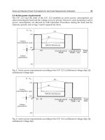
substation C will be deeply in systems A and B. Figure 21 shows the course of error level of
estimated resistance and reactance in protections located in the substations A and C in
relation to the WF generated power.
When the duration of a fault is so long that the control units of WF are coming into action,
the error level of impedance components evaluation for protections in the station C is still
rising. This is the consequence of the reduction of WF participation in the total fault current.
From Turbine to Wind Farms - Technical Requirements and Spin-Off Products

156
Figure 22 shows the change of the quotient of steady fault currents flowing from substations
A and C in relation to WF generated power P
WF
.

60

54

48

42

36
30
24
18
12
6
0,000

0,500

1,000

1,500

2,000

[Ω]

W
F Power [MW]
Δ
R(A)
Δ

X(A)
60
54
48
42
36
30
24
18
12

6
0,000
50,000
100,000
150,000
200,000
250,000
300,000
350,000
[Ω]
W
F Power [MW]
ΔR(C)
ΔX(C)

Fig. 21. Impedance components estimation errors in relation to WF generated power for
protections a) in substation A, b) in substation C

Fig. 22. Change of the quotient of steady fault currents flowing from sources B and C in
relation of WF generated power
Example 3

Once again the network is operating as in Figure 17. There are quasi-steady conditions, WF
is generating the nominal power of 60 MW, the fault point is at 90 % of the LA-B length. The
changing parameter is the location of WF connection point. It is changing from 3 to 24 km
from substation A.
Also for these conditions a higher influence of WF connection point location on the proper
functioning of power protections can be observed in substation C than in substations A and
B. The further the connection point is away from substation A, the lower are the error levels
of estimated impedance components in substations A and C. It is the consequence of the
rise of WF participation in the initial fault current (Table 4). The error levels for protections
in substation A are almost together, whereas in substation C they are many times lower than
in the case of a change in the WF generated power. If the fault time is so long that the
Quotient of short-circuit powers of sources A and C
0,000
10,000
20,000
30,000
40,000
50,000
60,000
70,000
80,000
90,000
60 54 48 42 36 30 24 18 12
6
WF Power [MW]
Distance Protections in the Power System Lines with Connected Wind Farms

157
control units of WF will come into action, limiting the WF fault current, the error level for
protections in substation C will rise more. This is due to the quotient
() ()
A
uCu
II which is
leading to the rise of estimation error
()
()
()
A
u
MF
C
Cu
I
ZZ
I
Δ= .
Figure 23 shows the course of error of reactance estimation for the initial and steady fault
current for impedances evaluated by the algorithms implemented in protection in substation
C.

WF connection
point location
A
I
C

I
CA
II
AC
II
ΔR
(A)
ΔX
(A)
ΔR
(C)
ΔX
(C)
[km] [kA] [kA] [-]
[-]
[Ω] [Ω] [Ω] [Ω]
3 2.362 0.481 0.204 4.911 0.586 1.955 14.143 47.142
6 2.371 0.525 0.221 4.516 0.558 1.860 11.381 37.936
9 2.385 0.57 0.239 4.184 0.516 1.721 9.038 30.126
12 2.402 0.617 0.257 3.893 0.462 1.541 7.007 23.358
15 2.424 0.6652 0.274 3.644 0.395 1.317 5.247 17.491
18 2.45 0.716 0.292 3.422 0.316 1.052 3.696 12.318
21 2.48 0.769 0.310 3.225 0.223 0.744 2.322 7.740
24 2.518 0.825 0.328 3.052 0.118 0.393 1.099 3.663
Table 4. Values and quotients of the initial fault currents flowing from sources A and C, and
the error levels of impedance components estimation in relation to the WF connection point
location


Error levels of reactance estimation for protection in substation C

0

100

200

300

400

500

600

700

800

3 6 9 12 15 18 21 24
W
F connection point [km]
[%]

Initial fault current Stead
y
fault current

Fig. 23. Error level of the reactance estimation for distance protection in substation C in
relation of WF connection point
From Turbine to Wind Farms - Technical Requirements and Spin-Off Products

158
Taking the network structure shown in Fig. 24, according to distance protection principles,
the reach of the first zone should be set at 90 % of the protected line length. But in this case,
if the first zone is not to reach the busbars of the surrounding substations, the maximum
reactance settings should not exceed:
For distance protection in substation A:
(
)
Ω
=
+
<
28.02.1
1A
X
For distance protection in substation B:
(
)
Ω
=
+
<
6.118.08.10
1B
X
For distance protection in substation C:
(
)
Ω

=
+
<
28.02.1
1C
X
With these settings most of the faults on segment L
MB
will not be switched off with the self-
time of the first zone of protection in substation A. This leads to the following switching-off
sequence. The protection in substation B will switch off the fault immediately. The network
will operate in configuration with two sources A and C. If the fault has to be switched off
with the time Δt, the reaches of second zones of protections in substations A and C have to
include the fault location. So their reach must extend deeply into the system A and the WF
structure. Such a solution will produce serious problems with the selectivity of functioning
of power protection automation.
Taking advantage of the in-feed factor k
if
also leads to a significant extension of these zones,
especially for protection in substation C. Due to the highly changeable value of this factor in
relation to the WF generated power and the location of connection, what will be efficient is
only adaptive modified settings, according to the operating conditions identified in real
time.


WF
S
y
stem B
S

y
ste
m
A
A
C
M
B
(
)
Ω
+
=
8.024.0 jZ
LCM
()
Ω
+
=
8.1024.3 jZ
LMB
()
Ω
+
= 2.136.0 jZ
LAM

Fig. 24. Simplified impedance scheme of the network structure from the Figure 17
6. Conclusions
The presented selected factors influencing the estimation of impedance components in

digital protections, necessitate working out new protection structures. These must have
strong adaptive abilities and the possibility of identification, in real time, of an actual
operating state (both configuration of interconnections and parameters of work) of the
network structure. The presented simulations confirm that the classic parameterization of
distance protections, even the one taking into account the in-feed factor k
if
does not yield
effective and selective fault eliminations.
Nowadays distance protections have individual settings for the resistance and reactance
reaches. Thus the approach of the resistance reach and admitted load area have to be taken
Distance Protections in the Power System Lines with Connected Wind Farms

159
into consideration. Resistance reach should include faults with an arc and of high
resistances. This is at odds with the common trend of using high temperature low sag
conductors and the thermal line rating, which of course extends the impedance area of
admitted loads. As it has been shown, also the time of fault elimination is the problem for
distance protections in substations in the WF surrounding, when this time is so long that the
WF fault current is close to their nominal current value.
Simulation results prove that the three-terminal line type of DPGS connection, especially
wind farms, to the distribution network contributes to the significant shortening of the
reaches of distance protections. The consequences are:
•
extension of fault elimination time (switching off will be done with the time of the
second zone instead of the self-time first zone),
•
incorrectness of autoreclosure automation functioning (e.g. when in the case of
shortening of reaches the extended zones will not include the full length of line),
•
no reaction of protections in situations when there is a fault in the protected area

(missing action of protection) or delayed cascaded actions of protections.
A number of factors influencing the settings of distance protections, with the presence of
wind farms, causes that using these protections is insufficient even with pilot lines. So new
solutions should be worked out. One of them is the adaptive area automation system. It
should use the synchrophasors technique which can evaluate the state estimator of the local
network, and, in consequence, activates the adapted settings of impedance algorithms to the
changing conditions. Due to the self-time of the first zones (immediate operation) there is a
need for operation also in the area of individual substations. Thus, it is necessary to work
out action schemes in the case of losing communication within the dispersed automation
structure.
7. References
Datasheet: Vestas, Advance Grid Option 2, V52-850 kW, V66-1,75 MW, V80-2,0 MW, V90-
1,8/2,0 MW, V90-3,0 MW.
Halinka, A.; Sowa, P. & Szewczyk M. (2006): Requirements and structures of transmission
and data exchange units in the measurement-protection systems of the complex
power system objects. Przegląd Elektrotechniczny (Electrical Review), No. 9/2006, pp.
104 – 107, ISSN 0033-2097 (in Polish)
Halinka, A. & Szewczyk, M. (2009): Distance protections in the power system lines with
connected wind farms, Przegląd Elektrotechniczny (Electrical Reviev), R 85, No.
11/2009, pp. 14 – 20, ISSN 0033-2097 (in Polish)
Lubośny, Z. (2003): Wind Turbine Operation in Electric Power Systems. Advanced Modeling,
Springer-Verlag, ISBN: 978-3-540-40340-1, Berlin Heidelberg New York
Pradhan, A. K. & Geza, J. (2007): Adaptive distance relay setting for lines connecting wind
farms. IEEE Transactions on Energy Conversion, Vol 22, No.1, March 2007, pp. 206-
213
Shau, H.; Halinka, A. & Winkler, W. (2008): Elektrische Schutzeinrichtungen in Industrienetzen
und –anlagen. Grundlagen und Anwendungen, Hüting & Pflaum Verlag GmbH & Co.
Fachliteratur KG, ISBN 978-3-8101-0255-3, München/Heidelberg (in German)
Ungrad, H.; Winkler, W. & Wiszniewski A. (1995): Protection techniques in Electrical Energy
Systems, Marcel Dekker, Inc., ISBN 0-8247-9660-8, New York

From Turbine to Wind Farms - Technical Requirements and Spin-Off Products

160
Ziegler, G. (1999): Numerical Distance Protection. Principles and Applications, Publicis MCD,
ISBN 3-89578-142-8
8
Impact of Intermittent Wind Generation on
Power System Small Signal Stability
Libao Shi
1
, Zheng Xu
1
, Chen Wang
1
, Liangzhong Yao
2
and Yixin Ni
1

1
Graduate School at Shenzhen, Tsinghua University Shenzhen 518055,
2
Alstom Grid Research & Technology Centre, Stafford, ST17 4LX,
1
China
2
United Kingdom
1. Introduction
In recent years, the increasing concerns to environmental issues demand the search for more
sustainable electrical sources. Wind energy can be said to be one of the most prominent

renewable energy sources in years to come (Ackermann, 2005). And wind power is
increasingly considered as not only a means to reduce the CO
2
emissions generated by
traditional fossil fuel fired utilities but also a promising economic alternative in areas with
appropriate wind speeds. Albeit wind energy currently supplies only a fraction of the total
power demand relative to the fossil fuel fired based conventional energy source in most
parts of the world, statistical data show that in Northern Germany, Denmark or on the
Swedish Island of Gotland, wind energy supplies a significant amount of the total energy
demand. Specially it should be pointed out that in the future, many countries around the
world are likely to experience similar penetration levels. Naturally, in the technical point of
view, power system engineers have to confront a series of challenges when wind power is
integrated with the existing power system. One of important issues engineers have to face is
the impact of wind power penetration on an existing interconnected large-scale power
system dynamic behaviour, especially on the power system small signal stability. It is
known that the dynamic behavior of a power system is determined mainly by the
generators. So far, nearly all studies on the dynamic behavior of the grid-connected
generator under various circumstances have been dominated by the conventional
synchronous generators world, and much of what is to be known is known. Instead, the
introduction of wind turbines equipped with different types of generators, such as doubly-
fed induction generator (DFIG), will affect the dynamic behaviour of the power system in a
way that might be different from the dominated synchronous generators due to the
intermittent and fluctuant characteristics of wind power in nature. Therefore, it is necessary
and imperative to study the impact of intermittent wind generation on power system small
signal stability.
It should be noticed that most published literature are based on deterministic analysis which
assumes that a specific operating situation is exactly known without considering and
responding to the uncertainties of power system behavior. This significant drawback of
deterministic stability analysis motivates the research of probabilistic stability analysis in
which the uncertainty and randomness of power system can be fully understood. The

From Turbine to Wind Farms - Technical Requirements and Spin-Off Products

162
probabilistic stability analysis method can be divided into two types: the analytical method,
such as point estimate method (Wang et al., 2001); and the simulation method, such as
Monte Carlo Simulation (Rueda et al., 2009). And most published literature related to
probabilistic stability analysis are based on the uncertainty of traditional generators with
simplified probability distributions. With increasing penetration levels of wind generation,
and considering that the uncertainty is the most significant characteristic of wind
generation, a more comprehensive probabilistic stability research that considering the
uncertainties and intermittence of wind power should be conducted to assess the influence
of wind generation on the power system stability from the viewpoint of probability.
Generally speaking, the considered wind generation intermittence is caused by the
intermittent nature of wind source, i.e. the wind speed. Correspondingly, the introduction
of the probability distribution of the wind speed is the key of solution. In our work, the well-
known Weibull probability density function for describing wind speed uncertainty is
employed. In this chapter, according to the Weibull distribution of wind speed, the Monte
Carlo simulation technique based probabilistic small signal stability analysis is applied to
solve the probability distributions of wind farm power output and the eigenvalues of the
state matrix.
2. Wind turbine model
In modelling turbine rotor, there are a lot of different ways to represent the wind turbine.
Functions approximation is a way of obtaining a relatively accurate representation of a wind
turbine. It uses only a few parameters as input data to the turbine model. The different
mathematical models may be more or less complex, and they may involve very different
mathematical approaches, but they all generate curves with the same fundamental shapes as
those of a physical wind turbine.
In general, the function approximations representing the relation between wind speed and
mechanical power extracted from the wind given in Equation (1) (Ackermann, 2005) are
widely used in modeling wind turbine.

3
0
0.5 ( , )
0
wcutin
wt
p
wcutinwrated
m
rratedwcutoff
wcutoff
VV
AC V V V V
P
pVVV
VV
ρβλ
−
−
−
−
≤
⎧
⎪
⋅⋅ ⋅ ⋅ < ≤
⎪
=
⎨
<<

⎪
⎪
≥
⎩
(1)
where P
m
is the power extracted from the wind; ρ is the air density; C
p
is the performance
coefficient; λ is the tip-speed ratio (v
t
/v
w
), the ratio between blade tip speed, v
t
(m/s), and
wind speed at hub height upstream of the rotor, v
w
(m/s); A
wt
=πR
2
is the area covered by the
wind turbine rotor, R is the radius of the rotor; V
w
denotes the wind speed; and β is the
blade pitch angle; V
cut-in
and V

cut-offt
are the cut-in and cut-off wind speed of wind turbine;
V
rated
is the wind speed at which the mechanical power output will be the rated power.
When V
w
is higher than V
rated
and lower than V
cut-off
, with a pitch angle control system, the
mechanical power output of wind turbine will keep constant as the rated power.
It is known that the performance coefficient C
p
is not a constant. Usually the majority of
wind turbine manufactures supply the owner with a C
p
curve. The curve expresses C
p
as a
function of the turbine’s tip-speed ratio λ. However, for the purpose of power system
Impact of Intermittent Wind Generation on Power System Small Signal Stability

163
stability analysis of large power systems, numerous researches have shown that C
p
can be
assumed constant. Fig. 1 (Akhmatov, 2002) gives the curves of performance coefficient C
p

with changing of rotational speed of wind turbine at different wind speed conditions (βis
fixed). According to Fig. 1, by adjusting the rotational speed of the rotor to its optimized
value
ω
m-opt
, the optimal performance coefficient C
pmax
can be reached.


Fig. 1. Curves of C
p
with changing of
ω
m
at different wind speed
In this chapter, we assume that for any wind speed at the range of V
cut-in
< V
w
≤V
rated
, the
rotational speed of rotor can be controlled to its optimized value, therefore the C
pmax
can be
kept constant.
3. Mathematical model of DFIG
The configuration of a DFIG, with corresponding static converters and controllers is given in

Fig.1. Two converts are connected between the rotor and grid, following a back to back
scheme with a dc intermediate link. Fig.2 gives the reference frames, where a, b and c
indicate stator phase a, b and c winding axes; A, B and C indicate rotor phase A, B and C
winding axes, respectively; x-y is the synchronous rotation coordinate system in the grid
side; θ is the angle between q axis and x axis.
Applying Park’s transformation, the voltage equations of a DFIG in the d-q coordinate
system rotating at the synchronous speed
ω
s
, in accordance with generator convention,
which means that the stator and rotor currents are positive when flowing towards the
network, and real and reactive powers are positive when fed into grid, can be deducted as
follows in a per unit system.

1
ds
ds s ds qs
s
d
URI
dt
ψ
ψ
ω
=− − + (2)
From Turbine to Wind Farms - Technical Requirements and Spin-Off Products

164

Fig. 2. Schematic diagram of DFIG with converters and controllers

Fig. 3. Reference coordinates for DFIG

1
q
s
qs s qs ds
s
d
URI
dt
ψ
ψ
ω
=− + + (3)

1
dr
dr r dr qr
s
d
URIs
dt
ψ
ψ
ω
=− − + (4)

1

q
r
qr r qr dr
s
d
URIs
dt
ψ
ψ
ω
=− + + (5)
P
g
,Q
g

P
g
+jQ
g

G
I
r

I
s

P
r

U
s
U
t

controller
P
s

Impact of Intermittent Wind Generation on Power System Small Signal Stability

165

ds s ds m dr
XI X I
ψ
=
−− (6)

q
ss
q
sm
q
r
XI X I
ψ
=
−− (7)

dr r dr m ds
XI X I
ψ
=
−− (8)

q
rr
q
rm
q
s
XI X I
ψ
=
−− (9)

()()
g
s r ds ds
q
s
q
sdrdr
q
r
q
r
PPPUI UI UI UI

=
+= + + + (10)

()()
g
sr
q
sds ds
q
s
q
rdr dr
q
r
QQQ UI UI UI UI
=
+= − + −
(11)

2
em
ds
HTT
dt
=
−
(12)
Where U, I, Ψ denote the voltage, current and flux linkage; P and Q denote the real and
reactive power outputs of wind generator, respectively; T
m

and T
e
denote the mechanical
and electromagnetic torques of wind generator, respectively; R and X denote resistance and
reactance, respectively; the subscripts r and s denote the stator and rotor windings,
respectively; the subscript g means generator; H is the inertia constant, and t stands for time;
s is the slip of speed.
The reactances X
s
and X
r
can be calculated in following equations.

ss m
XX X
σ
=
+ (13)

rr m
XX X
σ
=+ (14)
Where X
s
σ
and X
r
σ
are the leakage reactances of stator and rotor windings, respectively; X

m

is the mutual reactance between stator and rotor.
The aforementioned equations describe the electrical dynamic performance of a wind
turbine, namely, the asynchronous machine. However, these equations are not suitable for
small signal analysis directly. It is necessary and imperative to deduce the simplified and
practical model. The following assumptions are presented to model the DFIG.
a.
Magnetic saturation phenomenon is not considered during modelling;
b.
For the wind turbine equipped with DFIG, all rotating masses are represented by one
element, which means that a so-called ‘lumped-mass’ or ‘one-mass’ representation is
used;
c.
The stator transients and stator resistance are negligible, i.e.
0
ds
d
dt
ψ
=
, 0
qs
d
dt
ψ
= , and
R
s
=0 in Eqs (2) and (3).

Furthermore, the stator flux-oriented control strategy (Tapia et al., 2006) is adopted in this
work, which makes the stator flux
ψ
s
line in accordance with d-axis, as depicted in Fig.3., i.e.

ssd
ψ
ψ
=
(15)

s
0
q
ψ
=
(16)
From Turbine to Wind Farms - Technical Requirements and Spin-Off Products

166
Then the stator voltage equations can be rewritten as

0
ds
U
=
(17)

sstq

UU
ψ
=
= (18)
Where U
t
is the terminal voltage;
From Fig. 3, the vector of stator voltage U
s
=U
t
is always align with q axis with the stator
flux-oriented control strategy. And according to the stator flux linkage equations (6) and (7),
the stator currents I
ds
and I
qs
can be represented as the function of rotor current and terminal
voltage U
t
, i.e.

1
()
ds t m dr
s
IUXI
X
=− + (19)

1
q
sm
q
r
s
IXI
X
=− (20)
Substituting equations (8) and (9) in equations (4) and (5), we find

rdr
dr r dr r
q
r
s
XdI
URI sXI
dt
ω
′
′
=− − + (21)

qr
rm
q
rr
q
rrdrs

ss
dI
XX
URI sXIs
dt X
ψ
ω
′
′
=− − − +
(22)
Where X
r
’=X
r
-X
m
2
/X
s.

Consider that the grid-side converter of DFIG always operates at unity power factor, i.e.
Q
r
= 0, the reactive power Q
g
is equal to the stator reactive power Q
s
, i.e. Q
g

=Q
s
. In the steady
state analysis, in accordance with the expressions of stator power and the rotor power, it can
be proved that P
r
=-sP
s
, and P
g
=P
s
/(1-s). Accordingly, the real and reactive powers equations
and the torque equation can be rewritten as

/(1 )
(1 )
t
g
sm
q
r
s
U
PP s XI
Xs
=−=−
−
(23)

()
t
g
stmdr
s
U
QQ UXI
X
==− + (24)

2()
m
em ds
q
s
q
sds m t
q
rm
s
X
ds
HTT I IT UIT
dt X
ψψ
=− = + − =− − (25)
Finally, the equations (17-18), (21-22), (23-25) constitute the 3
rd
order simplified practical
DFIG model.

4. Mathematical model of DFIG Converters
As shown in Fig.2, the model of DFIG frequency converter system consists of rotor-side
converter, grid-side converter, the dc link and the corresponding converter control. In this
Impact of Intermittent Wind Generation on Power System Small Signal Stability

167
chapter, it is assumed that the grid-side converter is ideal and the dc link voltage between
the converters is constant during analysis. This decouples the grid-side converter from the
rotor-side converter. The rotor-side converter is assumed to be a voltage-controlled current
source, and the stator flux-oriented control strategy is employed to implement the
decoupled control of the real and reactive power outputs of DFIG. The overall converter
control system consists of two cascaded control loops, i.e. the inner control and the outer
control. The inner control loop implements the rotor current control, and the outer control
loop implements the power control (Tapia et al., 2006).
In order to implement the decoupled control of the real and reactive power outputs of DFIG,
two new variables,
ˆ
dr
U ,
ˆ
q
r
U are introduced which are defined as:

ˆ
dr dr r
q
r
UUsXI
′

=− (26)

ˆ
m
q
r
q
rrdr s
s
X
UUsXIs
X
ψ
′
=+ − (27)
The newly introduced variables can fully make the dynamics of d and q axes decoupling.
Accordingly, the rotor voltage equations can be rewritten as

ˆ
rdr
dr r dr
s
XdI
URI
dt
ω
′
=− − (28)

ˆ

q
r
r
qr r qr
s
dI
X
URI
dt
ω
′
=− −
(29)
In this chapter, two special PI controllers are designed to implement the decoupled control
of the real and reactive power outputs of DFIG. The block diagrams of rotor-side converter
including the inner and outer control loops expressed in d and q axes are given in Fig.4 and
Fig.5. In the rotor current control loop, T
r
’=X
r
’/R, T
r
’ is the time constant of rotor circuit; I
drref
,
I
qrref
are the rotor current references in d and q axes, respectively; K
2
and T

2
are the control
parameters of PI controller. In the power control loop, P
sref
, Q
sref
are the real and reactive
power references; K
1
, T
1
are the control parameters of PI controller. It should be noted that
the specific values of K
1
, T
1
, K
2
and T
2
can be determined through pole placement method
(Tapia et al., 2006).
In accordance with Fig. 4, the corresponding stator real power control model can be
described as

111 1
()()
qrref sref
s
ssre

f
dI dP
dP
TKT KPP
dt dt dt
−−=− (30)

222 2
ˆ
()()
qr qr qrref
q
r
q
rre
f
dU dI dI
TKT KII
dt dt dt
+−=−
(31)

ˆ
q
r
q
r
r
qr
sr

dI U
T
I
dt R
ω
′
=− − (32)
From Turbine to Wind Farms - Technical Requirements and Spin-Off Products

168
1
1
K
Ts
2
2
K
Ts
sr
r
sT
R
ω
/1
/1
′
+
s
mt
X

XU
−
sref
P−
s
P−
qr
U
ˆ
1
K
2
K
qrref
I
−
qr
I−

Fig. 4. Block diagram of real power control system in rotor-side converter

1
1
K
Ts
2
2
K
Ts
sr

r
sT
R
ω
/1
/1
′
+
m
X
st
XU /−
dr
I−
sref
Q−
dr
U
ˆ
t
U
s
Q−
1
K
2
K
drref
I
−

Fig. 5. Block diagram of reactive power control loop in rotor-side converter

s
sm
q
r
s
PXI
X
ψ
=− (33)
Similarly, the corresponding stator reactive power control model can be described as

111 1
()()
drref sref
s
ssre
f
dI dQ
dQ
TKT KQQ
dt dt dt
−−=− (34)

222 2
ˆ
()()
drref

dr dr
dr drre
f
dI
dU dI
TKT KII
dt dt dt
+−=− (35)

ˆ
rdr dr
dr
sr
TdI U
I
dt R
ω
′
=− − (36)