Six Sigma Projects and Personal Experiences Part 12 pptx
Bạn đang xem bản rút gọn của tài liệu. Xem và tải ngay bản đầy đủ của tài liệu tại đây (462.93 KB, 15 trang )
Six Sigma Projects and Personal Experiences
156
Fig. 4. Schematic total variation in manufacturing
%of total variation:
RR
product R R
GageR R
GR R
TV
&
22
&
&
% & 100 100 (3)
% contribution to total variance:
RR
oduct R R
GageR R
Contribution GR R
TV
2
2
&
222
Pr &
&
% ( & ) 100 100 (4)
These metrics give an indication of how capable the gage is for measuring the critical to
quality characteristic. Acceptable regions of gage R&R as defined by the Automotive
Industry Action Group (Measurement Systems Analysis Workgroup, Automotive Inductry
Action Group, 1998) are as indicated in table 2.
GAGE R&R RANGE ACTION REQUIRED
<10% Gage acceptable
10% < Gage R&R < 30% Action required to understand variance
30% < Gage R&R
Gage unacceptable for use and
requires improvement
Table 2. Acceptable regions of Gage R&R.
Note that similar equations can be written for the individual components of variance and
also for the product contribution by replacing
R&R
with
repeatability
,
reproducibility
and
product
respectively.
Once the MSA indicates that the measurement method is both sufficiently accurate and
capable, it can be integrated into the remaining steps of the DMAIC process to analyse,
improve and control the characteristic.
3. Review of existing methodologies employed for MSA
Historically gages within the manufacturing enviornment have been manual devices
capable of measuring one single critical to quality characteristic. Here the components of
Gage Repeatability and Reproducibility Methodologies
Suitable for Complex Test Systems in Semi-Conductor Manufacturing
157
variance are (a) the repeatability on a given part, and (b) the reproducibility across operators
or appraiser effect. To estimate the components of variance in this instance, a small sample
of readings is required by independent appraisers. Typical data collection operations
comprised of 5 parts measured by each of 3 appraisers.There are three widely used methods
in use to analyse the collected data. These are the range method, the average and range
method, and the analysis of variance (ANOVA) method (Measurement Systems Analysis
Workgroup, Automotive Inductry Action Group, 1998).
The range method utilises the range of the data collected to generate an estimate of the
overall variance. It does not provide estimates of the variance components. The average and
range method is more comprehensive in that it utilises the average and range of the data
collected to provide estimates of the overall variance and the components of variance i.e. the
repeatability and reproducibility. The ANOVA method is the most comprehensive in that it
not only provides estimates of the overall variance and the components of variance, it also
provides estimates of the interaction between these components. In addition, it enables the
use of statistical hypothesis testing on the results to identify statistically significant effects.
ANOVA methods capable of replacing the range / average and range methods have
previously been described (Measurement Systems Analysis Workgroup, Automotive
Inductry Action Group, 1998). A relative comparison of these three methods are
summarised in table 3 below.
METHOD ADVANTAGE DISADVANTAGE
Range method.
Simple calculation
method.
Estimates overall variance
only - excludes estimate of
the components of R&R.
Average and range method.
Simple calculation
method.
Enables estimate of overall
variance and component
variance.
Estimates overall variance
and components but
excludes estimate of
interaction effects.
ANOVA method.
Enables estimates of
overall variance and all
components including
interaction terms.
More accuracy in the
calculated estimates.
Enables statistical
hypothesis testing.
Detailed calculations -
require automation.
Table 3. Compare and contrast historical methods for Gage R&R
The metrics generated from these gage R&R studies are typically the percentage total
variance and the percentage contribution to total variance of the repeatability, the
reproducibility or appraiser effect, and the product effect. A typical gage R&R results table
is shown in table 4.
With increasing complexity in semiconductor test manufacturing, automated test equipment
is used to generate measurement data for many critical to quality characteristic on any given
product. Additional sources of test variance can be recognised within this complex test
system. More advanced ANOVA methods are required to enable MSA in this situation.
Six Sigma Projects and Personal Experiences
158
Note that for cycle time and cost reasons, the data collection steps have an additional
constraint in that the number of experimental runs must be minimised. Design of
experiments is used to achieve this optimization.
Estimate of
Variance
component
Standard Deviation
% of Total Variation % Contribution.
Equipment
Variation or
Repeatability.
Equipment
Variaiton (EV)
=
repetability
22
&
100
repeatability
product R R
2
22
&
100
repeatability
product R R
Appraiser or
Operator
Variation.
Appraiser Variation
(AV)
=
reproducibility
22
&
100
reproducibility
product R R
2
22
&
100
reproducibility
product R R
Interaction
variation.
Appraiser by
product interaction
=
interaction
22
&
100
Interaction
product R R
2
22
&
100
Interaction
product R R
System or
Gage
Variation.
Gage R&R
=
R&R
&
22
&
100
RR
product R R
2
&
22
&
100
RR
product R R
Product
Variation.
Product variation
(PV) =
product
22
&
100
product
product R R
2
22
&
100
product
product R R
Table 4. Measurement systems analysis metrics evaluating Gage R&R.
4. MSA for complex test systems
With increased complexity and cost pressure within the semiconductor manufacture
environment, the test equipment used is automated and often tests multiple devices in
parallel. This introduces additional components of variance of test error. These are illustrated
in figure 5. The components of variance in this instance can be identified as follows.
Fig. 5. Components of test variance in manufacturing-System, Boards, Sites
Gage Repeatability and Reproducibility Methodologies
Suitable for Complex Test Systems in Semi-Conductor Manufacturing
159
The test repeatability or replicate error is the variance seen on one unit on one test set-up.
Because test repeatability may vary across the expected device performance window i.e. a
range effect, multiple devices from across the expected range are used in the investigation of
test repeatability error.
As the test operation is fully automated, the traditional appraiser affect is replaced by the
test setup reproducibility. The test reproducibility therefore comes from the physical
components of the test system setup. These are identified as the testers and the test boards
used on the systems. In addition, when multi-site testing is employed allowing testing of
multiple devices in parallel across multiple sites on a given test board, the test sites
themselves contribute to test reproducibility.
In investigating tester to tester and board to board effects a fixed number of specific testers
and boards will be chosen from the finite population of testers and boards. Because these are
being specifically chosen, a suitable experimental design in this case is a Fixed Effects Model
in which the fixed factors are the testers and the boards.
In investigating multisite site-to-site effects, the variation across the devices used within the
sites is confounded with the site-to-site variation. The devices used within the sites are
effectively a nuisance effect and need to be blocked from the site to site effects. In this
instance a suitable experimental design is a blocked design.
5. Fixed effects experimental design for test board and tester effects
In this instance there are two experimental factors – the test boards and the test systems. The
MSA therefore requires a two factor experimental design. For the example of two factors at
two levels, the data collection runs are represented by an array shown in table 5. To ensure
an appropriate number of data points are collected in each run, 30 repeats or replicates are
performed.
Run number Tester level Board level
1 1 1
2 1 2
3 2 1
4 2 2
Table 5. Experimental Array - 2 Factors at 2 Levels.
An example dataset is shown in figure 6. This shows data from a measurement on a
temperature sensor product. Data were collected from devices across two test boards and
two test systems. Both the tester to tester and board to board variations are seen in the plot.
5.1 Fixed effects statistical model
Because the testers and boards are chosen from a finite population of testers and boards, in
this instance a suitable statistical model is given by equation 5 (Montgomery D.C, 1996):
ijk i j ij ijk
Y ( ) e i 1 to t
j
1 to
b
k 1 to r
(5)
Six Sigma Projects and Personal Experiences
160
Fig. 6. Example data Fixed Effects Model- Across Boards and Testers.
Where Y
ijk
are the experimentally measured data points.
is the overall experimental mean.
i
is the effect of tester ‘i’.
j
is the effect of board ‘j’.
()
ij
is the interaction effect between testers and boards.
k is the replicate of each experiment.
e
ijk
is the random error term for each experimental measurement.
Here it is assumed that
i
,
j
, ()
ij
and e
ijk
are random independent variables, where {
i
}
~
N(0,
2
T
j
}~ N(0,
2
B
and {e
ijk
}~N(0,
2
R
The analysis of the model is carried out in two stages. The first partitions the total sum of
squares (SS) into its constituent parts. The second stage uses the model defined in equation 5
and derives expressions for the expected mean squares (EMS). By equating the SS to the
EMS the model estimates are calculated. Both the SS and the EMS are summarised in an
ANOVA table.
5.2 Derivation of expression for SS
The results of this data collection are represented by the generalized experimental result Y
hk,
where h= 1 … s is the total number of set-ups or experimental runs, and k= 1 … r is the
number of replicates performed on each experimental run. Using the dot notation, the
following terms are defined:
Set-up Total:
r
hhk
k
YY
.
1
denotes the sum of all replicates for a given set-up.
Overall Total:
sr
hk
hkYY
11
denotes the sum of all data points.
Overall Mean:
sr
hk
hkYYsr
11
/( ) denotes the average of all data points.
The effect of each factor is analysed using ‘contrasts’. The contrast of a factor is a measure of
the change in the
total of the results produced by a change in the level of the factor. Here a
simplified “-” and “+“ notation is used to denote the two levels. The contrast of a factor is
the difference between the sum of the set-up totals at the “+“ level of the factor and the sum
Gage Repeatability and Reproducibility Methodologies
Suitable for Complex Test Systems in Semi-Conductor Manufacturing
161
of the set-up totals at the “-” level of the factor. The array is rewritten to indicate the contrast
effects of each factor as shown in table 6.
Run
number
Tester
level
Board
level
Tester x Board
Interaction
Generalized Experimental
Result
1 - - +
Y
hk
, where:
h= 1 to s set-ups (= 4)
k= 1 to r replicates (= 30)
2 - + -
3 + - -
4 + + +
Table 6. Fixed Effects Array with 2 Level Contrasts
The contrasts are determined for each of the factors as follows:
Tester contrast
= -Y
1.
-Y
2.
+Y
3.
+Y
4.
Board contrast= -Y
1.
+Y
2.
-Y
3.
+Y
4.
Interaction contrast= +Y
1.
-Y
2.
-Y
3.
+Y
4.
The SS for each factor are written as:
Tester: SS
T
= [-Y
1.
- Y
2.
+ Y
3.
+ Y
4.
]
2
/ (sr) (6)
Board: SS
B
= [-Y
1.
+ Y
2.
- Y
3.
+ Y
4.
]
2
/ (sr) (7)
Interaction (TXS): SS
TxB
= [+ Y
1.
– Y
2.
–Y
3.
+ Y
4.
]
2
/ (sr) (8)
Total:
sr
hk
TOTAL
hk
SS Y Y sr
22
11
()/()
(9)
Residual: SS
R
= SS
TOTAL
– (SS
T
+ SS
B
+ SS
TxB
) (10)
5.3 Derivation of expression for EMS and ANOVA table
Expressions for the EMS of each factor are also needed. This is found by substituting the
equation for the linear statistical model into the SS equations and simplifying. In this case
the EMS are as follow.
Tester: EMS
T
=
2
R
+ r
2
TxB
+ br
2
T
(11)
Board: EMS
B
=
2
R
+ r
2
TxB
+ tr
2
B
(12)
Interaction : EMS
TXB
=
2
R
+ r
2
TxB
(13)
Residual: EMS
R
2
R
(14)
These EMS are equated to the MS from the experimental data and solved to find the
variance attributable to each factor in the experimental design.
The results of this analysis is summarised in an ANOVA table. The terms presented in this
ANOVA table are as follows. The SS are the calculated sum of squares from the
Six Sigma Projects and Personal Experiences
162
experimental data for each factor under investigation. The DOF are the degrees of freedom
associated with the experimental data for each factor. The MS is the mean square calculated
using the SS and DOF. The EMS is estimated mean square for each factor derived from the
theoretical model. For the design of experiment presented in this section the ANOVA table
is shown in table 7 below.
Source SS DOF MS EMS
Tester Eq. (6) t – 1 SS
T
/(t – 1)
2
R
+ r
2
TxB
+ br
2
T
Board Eq. (7) b – 1 SS
B
/(b – 1)
2
R
+ r
2
TxB
+ tr
2
B
Interaction Eq. (8) (t – 1)(b – 1) SS
TxB
/((t – 1)(b – 1))
2
R
+ r
2
TxB
Residual Eq. (10) tb(r – 1) SS
R
/(tb(r – 1))
2
R
Total Eq. (9) tbr – 1 Sum of above
Table 7. Fixed Effects ANOVA Table
5.4 Output of ANOVA – complete estimate of robust test statistics
Equating the MS from the experimental data to the EMS from the model analysis, it is
possible to solve for the variance estimate due to each source. From the ANOVA table the
best estimate for
x
and
R
are derived as S
2
T
, S
2
B
, S
2
TxB
and S
2
R
respectively. The
calculations on the ANOVA outputs to generate these estimates are listed in table 8.
Source Variance Estimate
Tester
S
T
=
TR TxB
MS r
br
22
Board
s
B
=
BR TxB
MS r
tr
22
Interaction
S
TxB
=
TxB R
MS
r
2
Residual
S
R
= MS
R
Total Sum of above
Table 8. Fixed Effects Model Results Table
Note that because each setup is measured a number of times on each device, the residual
contains the replicate or repeatability effect.
5.5 Example test data – experimental results
For the example dataset, there are two testers and two boards, hence t = b = 2. In addition
during data collection there were 30 replicates done on each site, hence r = 30. Using these
values and the raw data from the dataset, the ANOVA results are in tables 9 and 10
below.
Here the dominant source of variance is the test system variance, with S
T
= 0.403. This has a
P value < 0.01, indicating that this effect is highly significant. The variances from all other
sources are negligible in comparison, with S
2
R,
S
2
TXB,
S
B
variances of 0.015, 0.008, and 0.001
respectively.
Gage Repeatability and Reproducibility Methodologies
Suitable for Complex Test Systems in Semi-Conductor Manufacturing
163
Source SS DOF MS F P
Tester 24.465 1 24.465 1631 <0.01
Board 0.303 1 0.303 20.2 0.58
Interaction 0.243 1 0.243 15.2 0.62
Residual 1.791 116 0.015
Total 26.730 119 0.230
Table 9. Example Data - ANOVA Table Results
Source Variance Estimate
Tester
S
T
= 0.403
Board
S
B
= 0.001
Interaction
S
2
TxR
Residual
S
2
R
Total
S
T +
S
B +
S
2
TxR +
S
2
R
= 0.427
Table 10. Example Data - Calculation of Variances
6. Blocked experimental design for estimating multi-site test boards
For cost reduction, multisite test boards is employed allowing multiple parts to be tested in
parallel. In analysing the effect of each test site, the variance of the part is confounded into
the variance of the test site. In this instance the variability of the parts becomes a nuisance
factor that will affect the response. Because this nuisance factor is known and can be
controlled, a blocking technique is used to systematically eliminate the part effect from the
site effects.
Take the example of a quad site tester in which 4 parts are tested in 4 independent sites in
parallel. In this instance the variability of the parts needs to be removed from the overall
experimental error. A design that will accomplish this involves testing each of 4 parts
inserted in each of the 4 sites. The parts are systematically rotated across the sites during
each experimental run. This is in effect a blocked experimental design. The experimental
array for this example is shown in table 11, using parts labled A to D.
Run Site1 Site2 Site3 Site4
1 A B C D
2 B C D A
3 C D A B
4 D A B C
Table 11. Example Array Blocked Experimental Design.
An example dataset from a quad site test board is shown in figure 7. This shows data from a
temperature sensor product. Data were collected using 4 parts rotated across the 4 test sites
as indicated in the array above.
Six Sigma Projects and Personal Experiences
164
Fig. 7. Example data Blocked Experimental Design – Parts And Sites.
6.1 Blocked design statistical model
In this instance a suitable statistical model is given by equation 15 (Montgomery D.C, 1996):
ijk i j ij ijk
Y ( ) e i 1 to p
j
1 to s
k 1 to r
(15)
Where Y
ijk
are the experimentally measured data points.
is the overall experimental mean.
i
is the effect of device ‘i’.
j
is the effect of site ‘j’.
(
)
ij
is the interaction effect between devices and sites.
k is the replicate of each experiment.
e
ijk
is the random error term for each experimental measurement.
Here it is assumed that
i
,
j
, ()
ij
and e
ijk
are random independent variables, where {
i
}~
N(
2
P
j
} ~ N(0,
2
S
and {e
ijk
} ~
N(
2
R
As before, the analysis of the model is carried out in two stages. The first partitions the total
SS into its constituent parts. The second uses the model as defined and derives expressions
for the EMS. By equating the SS to the EMS the model estimates are calculated. Both the SS
and the EMS are summarised in an ANOVA table.
6.2 Derivation of expression for SS
The generalised experimental array is redrawn in the more general form in table 12.
Site 1 Site 2 Site 3 Site j Part Total
Part 1 Y
11k
Y
12k
Y
13k
Y
1
j
k
Y
1
Part 2 Y
21k
Y
22k
Y
23k
Y
2
j
k
Y
2
Part 3 Y
31k
Y
32k
Y
33k
Y
3
j
k
Y
3
Part i Y
i1k
Y
i2k
Y
i3k
Y
i
j
k
Y
i
Site Total Y
.1.
Y
.2.
Y
.3.
Y
.
j
.
Y
…
Table 12. Generalised Array – Blocked Experimental Design.
Gage Repeatability and Reproducibility Methodologies
Suitable for Complex Test Systems in Semi-Conductor Manufacturing
165
The results of this data collection are represented by the generalised experimental result Y
ijk
,
where i= 1 to p is the total number of parts, j= 1 to s is the total number of sites, and k= 1 to r
is the number of replicates performed on each experimental run.
Using the dot notation, the following terms are written:
Parts total:
sr
ii
j
k
jk
YY
11
is the sum of all replicates for each part.
Site total:
p
r
j ijk
ik
YY
11
is the sum of all replicates on a particular site.
Overall total:
p
sr
i
j
k
ijk
YY
111
is the overall sum of measurements.
The SS for each factor are written as:
Parts:
p
Pi
i
SS Y sr Y psr
22
1
/( ) /( ) (16)
Sites:
S
Sj
j
SS Y pr Y psr
22
1
/( ) /( ) (17)
Interaction:
pp
ss
PXS ij j i
ij j i
SS Y r Y pr Y sr Y psr
22 22
11 1 1
/( ) /( ) /( ) /( ) (18)
Total:
p
sr
TOTAL ijk
ijk
Y
SS Y
p
sr
2
2
111
(19)
Residual:
SS
R
= SS
TOTAL
– (SS
S
+ SS
P
+ SS
PxS
). (20)
6.3 Derivation of expression for EMS and ANOVA table
Expressions for the EMS for each factor are also needed. This is found by substituting the
equation for the linear statistical model into the SS equations and simplifying. In this case
the EMS are as follows.
Parts:
EMS
P
=
2
R
+ r
2
PxS
+ sr
2
P
(21)
Sites:
EMS
S
=
2
R
+ r
2
PxS
+ pr
2
S
(22)
Interaction:
Six Sigma Projects and Personal Experiences
166
EMS
PXS
=
2
R
+ r
2
PxS
(23)
Residual:
EMS
R
2
R
(24)
These are equated to the MS from the experimental data. These results for the blocked
experimental design are summarised in the ANOVA table shown in table 13.
Source SS DOF MS EMS
Parts Eq. (16) p – 1 SS
P
/(p – 1)
2
R
+ r
2
PxS
+ sr
2
p
Sites Eq. (17) s – 1 SS
S
/(s– 1)
2
R
+ r
2
PxS
+pr
2
S
Interaction Eq. (18) (s – 1)(p – 1) SS
PxS
/((s – 1)(p – 1))
2
R
+ r
2
PxS
Residual Eq. (20) sp(r – 1) SS
R
/(sp(r – 1))
2
R
Total Eq. (19) spr – 1
Table 13. ANOVA Table - Blocked Design.
6.4 Output of ANOVA – complete estimate of robust test statistics
Equating the MS from the experimental data to the EMS from the model analysis, it is
possible to solve for the variance due to each source. From the ANOVA table the best
estimate for
P
,
S
PxS
and
R
are derived as S
2
P
, S
2
S
, S
2
PxS
and S
2
R
respectively. The
calculations on the ANOVA outputs to generate these estimates are listed in table 14.
Source Variance Estimate
Parts
PR PxS
P
MS r
S
sr
22
2
Sites
SR PxS
S
MS r
S
pr
22
2
Interaction
PxS R
PXS
MS
S
r
2
2
Residual
RR
SMS
2
Table 14. Results Table – Blocked Design.
Note that because each setup is measured a number of times on each part, the residual
contains the replicate effect.
6.5 Example test data – experimental results
For the example from a quad site test board, there are 4 sites and 4 parts rotated across these
sites, hence s = p = 4. In addition during data collection there were 30 replicates done on
each site, hence r = 30. Using these values and the raw data from the dataset, the results of
the ANOVA are shown in tables 15 and 16.
Gage Repeatability and Reproducibility Methodologies
Suitable for Complex Test Systems in Semi-Conductor Manufacturing
167
Source SS DOF MS F p
Parts 0.063 3 0.021 2.6 0.05
Sites 8.800 3 2.933 366.6 <0.01
Interaction 9.414 9 1.04 130.0 <0.01
Residual 4.057 464 0.008
Total 22.335 479
Table 15. Example Data - ANOVA Table.
Source
Variance Estimate
Parts
S
P
= 0
Sites
S
S
= 0.021,
Interaction
S
PxS
= 0.035
Residual
S
R
= 0.009
Table 16. Example Data Calculation of Variance.
Here the dominant sources of variance are the test site variance, with S
S
= 0.021, and the
interaction variance estimate S
2
PxS =
0.015. Both these effects are highly significant with P
values < 0.01. The variances estimates from other sources are negligible in comparison, with
S
2
R,
S
P
of 0.009, and 0 respectively.
Figure 8 shows a replot of the original data with results grouped by site. It is clearly seen
that site 4 has an offset difference of about 0.2 compared to the other sites. It is primarily this
offset that is responsible for the site variance reported in the ANOVA.
Fig. 8. Temperature Sensor Offset – Replotted by Site.
7. Complete experimental design for MSA on quad site test system
For a complete MSA on a quad site test system both the fixed effects and blocked
experimental design are brought together. This enables optimisation within the data
collection stage. The complete experimental design is shown in table 17. Here four parts
are used – these are labelled A to D. These are rotated across the test sites in runs 1
through to 4. The data from these first 4 rows is analysed as a blocked experimental
design to estimate the site-to-site and part-to-part effects. In runs 5 to 7 a second test
Six Sigma Projects and Personal Experiences
168
board and test system are used to test the parts. The data from row 1 and rows 5 through
to 7 is analysed as a fixed experimental design to estimate the tester-to-tester and board-
to-board effects.
Run Tester Board Site 1 Site 2 Site 3 Site 4
1 1 1 A B C D
2 1 1 B C D A
3 1 1 C D A B
4 1 1 D A B C
5 1 2 A B C D
6 2 1 A B C D
7 2 2 A B C D
Table 17. Complete experimental design for quad site example
7.1 Complete experimental design for MSA on quad site test system
Example results obtained using this design of experiment are shown in table 18 and table 19
below. Table 18 presents the blocked design results, while table 19 presents the fixed design
results. Note that 30 repeats were done for each experimental run.
Source SS DOF MS F P
Tester 0.01199 1 0.01199 1.38 0.24
Board 0.01337 1 0.01337 1.54 0.21
Interaction 2.08E-05 116 1.79E-07 2.07E-05 1
Repeatability 1.031162 119 0.00866
Table 18. Fixed Factor Design Experimental Results.
Source SS DOF MS F P
Parts 4.1325 3 1.3775 152.30 <0.01
Sites 9.0550 3 3.0183 333.72 <0.01
Interaction 0.1653 9 0.0183 2.030 0.04
Repeatability 4.1966 464 0.0090
Table 19. Blocked Design Experimental Results.
From the ANOVA tables it is seen that both the sites and parts are statistically significant
with P values < 0.01, while the tester and board effects are not showing significance. The
variance estimates from both the fixed and blocked design are summarised in Table 20. The
total variance is obtained by summing the components of variance for both the fixed effects
design and the blocked design. The repeatability is taken as the largest value obtained from
either designs.
Gage Repeatability and Reproducibility Methodologies
Suitable for Complex Test Systems in Semi-Conductor Manufacturing
169
Source Variance Estimate
Fixed effects model results
Tester = S
T
5.18E-5
Board = S
B
7.47E-7
TXB = S
TXB
0.0000
Repeatability = S
R
Blocked design results
Parts = S
P
0.0226
Sites = S
S
0.0499
PXS = S
T
0.0031
Repeatability = S
R
0.0090
Test Gage R&R 0.0616
Total Variance (TV) = sum all components 0.0846
Table 20. Calculation of Components of Variances.
Using the equations (3) and (4) from section 2, the overall MSA metrics including gage R&R
results from these ANOVA are presented in table 21 .
Component
Variance
Estimate
Standard
Deviation
% Total
Variance
%Contribution to
variance
Components R&R :
Tester 5.18E-05 0.0071 2.4 0.06
Board 7.47E-07 0.0008 0.2 0.00
TesterXboard 0 0 0.0 0.00
Site 0.0499 0.2233 76.8 58.9
SiteXPart 0 0.0 0.00
Repeatability 0.0090 0.0948 32.6 10.6
Overall Gage R&R 0.0616 0.2481 85.3 72.8
Part 0.0226 0.1503 51.6 26.7
Total Variation 0.0846 0.2908 100.0 100
Table 21. Calculation of MSA metrics from experimental dataset.
8. Conclusions
Traditional measurement systems analysis methodologies are aimed at obtaining estimates
of test error components. These are identified as equipment repeatability and
reproducibility effects arising from independent appraisers. Gage R&R metrics can be
generated using the data gathered. The most commonly used metrics are the percentage of
total variation, and the percentage contribution to overall variance of each component.
With increasing complexity in semiconductor product test, the measurement equipment is
generally automated, and test boards are employed that are capable of testing multiple parts
in parallel. This introduces additional variance components not accounted for in these
traditional methodologies. These components are identified as the tester, board and test sites
effects. Updated ANOVA methodologies capable of accounting for this situation are
required to enable MSA.
Six Sigma Projects and Personal Experiences
170
The purpose of this chapter is to describe the appropriate experimental designs appropriate
for use in MSA in this situation. As the testers and boards come from a fixed population, a
suitable design of experiments for tester-to-tester and board-to-board effects is a fixed effects
experimental model. To evaluate site-to-site effects, the variation of the parts must be
blocked from the variation of the sites. A suitable design of experiments for site-to-site and
part-to-part effects is a blocked experimental design. Within this the parts are rotated across
the test sites to allow the independent variation of both the parts and the sites.
The derivations of the ANOVA tables for both designs are presented. The data collection
operation is optimised by merging the two designs. Experimental data gathered on a
product within a manufacturing environment is analysed using these designs, and the
results discussed. These designs enable the performance of MSA within the semiconductor
environment in a streamlined fashion.
9. References
Measurement Systems Analysis Workgroup, Automotive Industry Action Group, 2010.
Measurement and Systems Analysis Reference Manual.
Montgomery D.C, Runger G.C, (1993a)
“Guage Capability and Designs Experiments Part 1:
Basic Methods”,
Quality Engineering 6(2) 1993 115-135.
Montgomery D.C, Runger G.C (1993b) “Guage Capability and Designs Experiments Part I1:
Experimental Design Models and Variance Components Estimation”
. Quality
Engineering
6(2) 1093 289 – 305.
Montgomery D.C, (1996),
Design and Analysis of Experiments, Wiley Press, Fourth Edition.
Kubiak T.M, Benhow D.W (2009), The Certified Six-Sigma Handbook, ASQ Quality Press,
Second Edition.
Wheeler D., Lyday R., (1989),
Evaluating the Measurement Process, SPC Press.