Heat Transfer Mathematical Modelling Numerical Methods and Information Technology Part 14 pot
Bạn đang xem bản rút gọn của tài liệu. Xem và tải ngay bản đầy đủ của tài liệu tại đây (1.24 MB, 40 trang )
Heat Transfer at Microscale
509
(2005), which analytically studied fully developed natural convection in an open-ended
vertical parallel plate microchannel with asymmetric wall temperature distributions. They
showed that the Nusselt number based on the channel width is given by
1
12
2
(48)
where
and
are the wall temperatures and
is the free stream temperature. Chen and
Weng afterwards extended their works by taking the effects of thermal creep (2008a) and
variable physical properties (2008b) into account. Natural convection gaseous slip flow in a
vertical parallel plate microchannel with isothermal wall conditions was numerically
investigated by Biswal et al. (2007), in order to analyze the influence of the entrance region
on the overall heat transfer characteristics. Chakraborty et al. (2008) performed a boundary
layer integral analysis to investigate the heat transfer characteristics of natural convection
gas flow in symmetrically heated vertical parallel plate microchannels. It was revealed that
for low Rayleigh numbers, the entrance length is only a small fraction of the total channel
extent.
2.4 Thermal creep effects
When the channel walls are subject to constant temperature, the thermal creep effects
vanish at the fully developed conditions. However, for a constant heat flux boundary
condition, the effects of thermal creep may become predominant for small Eckert numbers.
Fig. 7. Variation of average Nusselt number as a function of the channel length, , for
different values of with 0.03 (Chen and Weng, 2008a)
The effects of thermal creep for parallel plate and rectangular microchannels have been
investigated by Rij et al. (2007) and Niazmand et al. (2010), respectively. As mentioned
before, Chen and Weng (2008a) studied the effects of creep flow in steady natural
Heat Transfer - Mathematical Modelling, Numerical Methods and Information Technology
510
convection in an open-ended vertical parallel plate microchannel with asymmetric wall heat
fluxes. It was found that the thermal creep has a significant effect which is to unify the
velocity and pressure and to elevate the temperature. Moreover, the effect of thermal creep
was found to be enhancing the flow rate and heat transfer rate and reducing the maximum
gas temperature and flow drag. Figure 7 shows the variation of average Nusselt number as a
function of the channel length, , for different values of with 0.03. Note that is
the ratio of the wall heat fluxes. It can be seen that the thermal creep significantly increases
the average Nusselt number.
3. Electrokinetics
In this section, we pay attention to electrokinetics. Electrokinetics is a general term
associated with the relative motion between two charged phases (Masliyah and
Bhattacharjee, 2006). According to Probstein (1994), the electrokinetic phenomena can be
divided into the following four categories
• Electroosmosis is the motion of ionized liquid relative to the stationary charged surface
by an applied electric field.
• Streaming potential is the electric field created by the motion of ionized fluid along
stationary charged surfaces.
• Electrophoresis is the motion of the charged surfaces and macromolecules relative to the
stationary liquid by an applied electric field.
• Sedimentation potential is the electric field created by the motion of charged particles
relative to a stationary liquid.
Due to space limitations, only the first two effects are being considered here. The study of
electrokinetics requires a basic knowledge of electrostatics and electric double layer.
Therefore, the next section is devoted to these basic concepts.
3.1 Basic concepts
3.1.1 Electrostatics
Consider two stationary point charges of magnitude
and
in free space separated by a
distance . According to the Coulomb’s law the mutual force between these two charges,
, is given by
F
4
r
(49)
in which
is a unit vector directed from
towards
. Here,
is the permittivity of
vacuum which its value is 8.854 10
CV
m
with C (Coulomb) being the SI unit of
electric charge. The electric field at a point in space due to the point charge is defined as
the electric force acting on a positive test charge
placed at that point divided by the
magnitude of the test charge, i.e.,
E
F
4
0
2
r
(50)
where is a unit vector directed from towards
. One can generalize Eq. (50) by
replacing the discrete point charge by a continuous charge distribution. The electric field
then becomes
Heat Transfer at Microscale
511
E
1
4
0
d
2
r
(51)
where the integration is over the entire charge distribution and
is the electrical charge
density which may be per line, surface, or volume.
Let us pay attention to the Gauss’s law, a useful tool which relates the electric field strength
flux through a closed surface to the enclosed charge. To derive the Gauss’s law, we consider
a point charge located in some arbitrary volume, , bounded by a surface as shown in
Fig. 8.
Fig. 8. Point charge bounded by a surface .
The electric field strength at the element of surface d due to the charge is given by
E
4
0
2
r (52)
where the unit vector is directed from the point charge towards
the surface element d.
Performing dot product for Eq. (52) using d with being the unit outward normal vector
to the bounding surface and integrating over the bounding surface S, we come up with
E · n
d
4
r · n
d
(53)
The term
·
d
2
⁄
represents the element of solid angle dΩ. Therefore, the above
equation becomes
E · n
d
1
4
0
d
4
0
(54)
Upon integration, Eq. (54) gives
E· n
d
(55)
Equation (55) is the integral form of the Gauss’s law or theorem. The differential form of the
Gauss’s law can be derived quite readily using the divergence theorem, which states that
E· n
d
·E
d
(56)
d
Heat Transfer - Mathematical Modelling, Numerical Methods and Information Technology
512
and the total charge may be written based on the
charge density as
d
(57)
The following equation is obtained, using Eqs. (55) to (57)
·E
d
1
d
(58)
Since the volume is arbitrary, therefore
· E
(59)
The above is the differential form of the Gauss’s law.
Using Eq. (50), it is rather straightforward to show that
E0
(60)
From the above property, it may be considered that the electric field is the gradient of some
scalar function, , known as electric potential, i.e.,
E
(61)
By substituting the electric field from Eq. (61) into Eq. (59), we come up with the Poison
equation:
(62)
Fig. 9. Polarization of a dielectric material in presence of an electric field
All the previous results are pertinent to the free space and are not useful for practical
applications. Therefore, we should modify them by taking into account the materials
no applied field
-
-
-
-
-
+
+
+
+ +
-
-
-
-
-
+
+
+
+ +
-
-
-
-
-
+
+
+
+ +
-
-
-
-
-
+
+
+
+ +
+
+
+
+
+
-
-
-
-
-
+
+
+
+
+
-
-
-
-
-
+
+
+
+
+
-
-
-
-
-
+
+
+
+
+
-
-
-
-
-
applied field,
Heat Transfer at Microscale
513
electrical properties. It is worth mentioning that from the perspective of classical
electrostatics, the materials are broadly categorized into two classes, namely, conductors
and dielectrics. Conductors are materials that contain free electric charges. When an
electrical potential difference is applied across such conducting materials, the free charges
will move to the regions of different potentials depending on the type of charge they carry.
On the other hand, dielectric materials do not have free or mobile charges. When a dielectric
is placed in an electric field, electric charges do not flow through the material, as in a
conductor, but only slightly shift from their average equilibrium positions causing dielectric
polarization. Because of dielectric polarization, positive charges are displaced toward the
field and negative charges shift in the opposite direction. This creates an internal electric
field that partly compensates the external field inside the dielectric. The mechanism of
polarization is schematically shown in Fig. 9.
Fig. 10. Schematic of a dipole.
We should now derive the relevant electrostatic equations for a dielectric medium. In the
presence of an electric field, the molecules of a dielectric material constitute dipoles. A
dipole, which is shown in Fig. 10, comprises two equal and opposite charges, and –,
separated by a distance . Dipole moment, a vector quantity, is defined as , where is the
vector orientation between the two charges. The polarization density, , is defined as the
dipole moment per unit volume. It is thus given by
Pd
(63)
where is the number of dipoles per unit volume. For homogeneous, linear, and isotropic
dielectric medium, when the electric field is not too strong, the polarization is directly
proportional to the applied field, and one can write
P
E
(64)
Here χ is a dimensionless parameter known as electric susceptibility of the dielectric
medium. The following relation exists between the polarization density and the volumetric
polarization (or bound) charge density,
·P
(65)
Within a dielectric material, the total volumetric charge density is made up of two types of
charge densities, a polarization and a free charge density
(66)
One can combine the definition of total charge density provided by Eq. (66) with the Gauss’s
law, Eq. (59), to get
Heat Transfer - Mathematical Modelling, Numerical Methods and Information Technology
514
·
1
(67)
By substituting the polarization charge, from Eq. (65), the divergence of the electric field
becomes
· E
1
· P
(68)
which may be rearranged as
·
E P
(69)
The polarization may be substituted from Eq. (64) and the outcome is the following
·
1
E
(70)
Let
1
(71)
We will call the permittivity of the material. Therefore, Eq. (70) becomes
·
E
(72)
For constant permittivity, Eq. (72) gives
· E
(73)
which is Maxwell’s equation for a dielectric material. Equation (73) may be written as
·E
(74)
with
1
being the relative permittivity of the dielectric material. The minimum
value of
is unity for vacuum. Its value varies from near unity for most gases to about 80
for water. Substituting for the electric field from Eq. (61), Eq. (73) becomes
(75)
Equation (75) represents the Poisson’s equation for the electric potential distribution in a
dielectric material.
3.1.2 Electric double layer
Generally, most substances will acquire a surface electric charge when brought into contact
with an electrolyte medium. The magnitude and the sign of this charge depend on the
physical properties of the surface and solution. The effect of any charged surface in an
electrolyte solution will be to influence the distribution of nearby ions in the solution, and
the outcome is the formation of an electric double layer (EDL). The electric double layer,
which is shown in Fig. 11, is a region close to the charged surface in which there is an excess
of counterions over coions to neutralize the surface charge. The EDL consists of an inner
layer known as Stern layer and an outer diffuse layer. The plane separating the inner layer
and outer diffuse layer is called the Stern plane. The potential at this plane,
, is close to the
Heat Transfer at Microscale
515
electrokinetic potential or zeta potential, which is defined as the potential at the shear
surface between the charged surface and the electrolyte solution. Electrophoretic potential
measurements give the zeta potential of a surface. Although one at times refers to a “surface
potential”, strictly speaking, it is the zeta potential that needs to be specified (Masliyah and
Bhattacharjee, 2006). The shear surface itself is somewhat arbitrary but characterized as the
plane at which the mobile portion of the diffuse layer can slip or flow past the charged
surface (Probstein, 1994).
Fig. 11. Structure of electric double layer
The spatial distribution of the ions in the diffuse layer may be related to the electrostatic
potential using Boltzmann distribution. It should be pointed out that the Boltzmann
distribution assumes the thermodynamic equilibrium, implying that it may be no longer
valid in the presence of the fluid flow. However, in most electrokinetic applications, the
Peclet number is relatively low, suggesting that using this distribution does not lead to
Debye length
diffuse la
y
er
Stern la
y
er
Stern plane
shear
char
g
ed surface
Heat Transfer - Mathematical Modelling, Numerical Methods and Information Technology
516
significant error. At a thermodynamic equilibrium state, the probability that the system
energy is confined within the range and d is proportional to d, and can be
expressed as
d with
being the probability density, given by
(76)
where is the absolute temperature and
1.3810
JK
⁄
is the Boltzmann constant.
Equation (76), initially derived by Boltzmann, follows from statistical considerations.
Here, corresponds to a particular location of an ion relative to a suitable reference state.
An appropriate choice may be the work required to bring one ion of valence
from
infinity, at which 0, to a given location having a potential . This ion, therefore,
possess a charge of
with 1.6 10
C being the proton charge. Consequently, the
system energy will be
and, as a result, the probability density of finding an ion at
location will be
(77)
Similarly, the probability density of finding the ion at the neutral state at which 0 is
(78)
The ratio of to
is taken as being equal to the ratio of the concentrations of the species
at the respective states. Combining Eqs. (77) and (78) results in
(79)
where
∞
is the ionic concentration at the neutral state and
is the ionic concentration of
the
ionic species at the state where the electric potential is . The valence number
can
be either positive or negative depending on whether the ion is a cation or an anion,
respectively. As an example, for the case of CaCl
2
salt, for the calcium ion is +2 and it is −1
for the chloride ion.
We are now ready to investigate the potential distribution throughout the EDL. The charge
density of the free ions,
, can be written in terms of the ionic concentrations and the
corresponding valances as
(80)
For the sake of simplicity, it is assumed that the liquid contains a single salt dissociating into
cationic and anionic species, i.e., 2. It is also assumed that the salt is symmetric
implying that both the cations and anions have the same valences, i.e.,
(81)
The charge density, thus, will be of the following form
(82)
or
Heat Transfer at Microscale
517
2
sinh
(83)
in which
∞
∞
∞
. Let us know consider the parallel plate microchannel which was
shown in Fig. 2. By introducing Eq. (83) into the Poisson’s equation, given by Eq. (75), the
following differential equation is obtained for the electrostatic potential
d
d
2
sinh
(84)
The above nonlinear second order one dimensional equation is known as Poisson-
Boltzmann equation. Yang et al. (1998) have shown with extensive numerical simulations
that the effect of temperature on the potential distribution is negligible. Therefore, the
potential field and the charge density may be calculated on the basis of an average
temperature,
. Using this assumption, Eq. (84) in the dimensionless form becomes
d
d
2
sinh
(85)
where
⁄
and
⁄
. The quantity
2
⁄
⁄
is the so-called
Debye length,
, which characterizes the EDL thickness. It is noteworthy that the general
expression for the Debye length is written as 2
∑
⁄
⁄
. Defining Debye-
Huckel parameter as 1
⁄
, we come up with
d
d
sinh
0
(86)
If
is small enough, namely
1, the term sinh
can be approximated by
. This
linearization is known as Debye-Huckel linearization. It is noted that for typical values of
298K and 1, this approximation is valid for 25.7mV. Defining dimensionless
Debye-Huckel parameter, , and invoking Debye-Huckel linearization, Eq. (86)
becomes
d
d
0
(87)
The boundary conditions for the above equation are
d
d
0 ,
(88)
in which
is the dimensionless wall zeta potential, i.e.,
⁄
. Using Eq. (87) and
applying boundary conditions (88), the dimensionless potential distribution is obtained as
follows
cosh
cosh
(89)
Heat Transfer - Mathematical Modelling, Numerical Methods and Information Technology
518
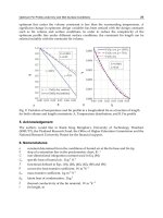
Figure 12 shows the transverse distribution of
at different values of
. The simplified
cases are those pertinent to the Debye-Huckel linearization and the exact ones are the results
of the Numerical solution of Eq. (86). The figure demonstrates that performing the Debye-
Huckel linearization does not lead to significant error up to
2 which corresponds to the
value of about 51.4 mV for the zeta potential at standard conditions. This is due to the fact
that for
2, the dimensionless potential is lower than 1 over much of the duct cross
section. According to Karniadakis et al. (2005), the zeta potential range for practical
applications is 1 100 mV, implying that the Debye-Huckel linearization may successfully
be used to more than half of the practical applications range of the zeta potential.
Fig. 12. Transverse distribution of
at different values of
3.2 Electroosmosis
As mentioned previously, there is an excess of counterions over coions throughout the EDL.
Suppose that the surface charge is negative, as shown in Fig. 13. If one applies an external
electric field, the outcome will be a net migration toward the cathode of ions in the surface
liquid layer. Due to viscous drag, the liquid is drawn by the ions and therefore flows
through the channel. This is referred to as electroosmosis. Electroosmosis has many
applications in sample collection, detection, mixing and separation of various biological and
chemical species. Another and probably the most important application of electroosmosis is
the fluid delivery in microscale at which the electroosmotic micropump has many
advantages over other types of micropumps. Electroosmotic pumps are bi directional, can
generate constant and pulse free flows with flow rates well suited to microsystems and can
be readily integrated with lab on chip devices. Despite various advantages of the
electroosmotic pumping systems, the pertinent Joule heating is an unfavorable
phenomenon. Therefore, a pressure driven pumping system is sometimes added to the
electroosmotic pumping systems in order to reduce the Joule heating effects, resulting in a
combined electroosmotically and pressure driven pumping.
Heat Transfer at Microscale
519
Fig. 13. A parallel plate microchannel with an external electric field
In the presence of external electric field, the poison equation becomes
(90)
The potential is now due to combination of externally imposed field Φ and EDL potential
, namely
Φ
(91)
For a constant voltage gradient in the direction, Eq. (90) is reduced to Eq. (84), and thus the
potential distribution is again given by Eq. (89). The momentum exchange through the flow
field is governed by the Cauchy’s equation given as
u
·τF
(92)
in which represents the pressure, and are the velocity and body force vectors,
respectively, and is the stress tensor. The body force is given by (Masliyah and
Bhattacharjee, 2006)
E
1
2
·ε
1
2
∂ε
∂
·
(93)
Therefore, for the present case, the body force is reduced to
, assuming a medium with
constant permittivity. Regarding that D D
⁄
0 at fully developed conditions, we come up
with the following expression for the momentum equation in the direction
d
d
d
d
2
sinh
(94)
Invoking the Debye-Huckel linearization, the dimensionless form of the momentum
equation becomes
d
d
2Γ
2Γ
cosh
cosh
(95)
in which
⁄
with
⁄
being the maximum possible electroosmotic
velocity for a given applied potential field, known as the Helmholtz-Smoluchowski
Heat Transfer - Mathematical Modelling, Numerical Methods and Information Technology
520
electroosmotic velocity. It is noteworthy that
⁄
is often termed the electroosmotic
mobility of the liquid. Also Γ is the ratio of the pressure driven velocity scale to
, namely
Γ
⁄
where
d d
⁄
2
⁄
. The boundary conditions for the momentum
equation are the symmetry condition at centerline and no slip condition at the wall. The
dimensionless velocity profile then is readily obtained as
Γ1
1
cosh
cosh
(96)
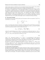
Dimensionless velocity profile for purely electroosmotic flow is depicted in Fig. 14. For a
sufficiently small value of such as 1, since EDL potential distribution over the duct
cross section is nearly uniform which is the source term in momentum equation (94), so the
velocity distribution is similar to Poiseuille flow. As dimensionless Debye-Huckel parameter
increases the dimensionless velocity distribution shows a behavior which is different from
Poiseuille flow limiting to a slug flow profile at sufficiently great values of . This is due to
the fact that at higher values of , the body force is concentrated in the region near the wall.
Fig. 14. Dimensionless velocity profile for purely electroosmotic flow
Dimensionless velocity profile at different values of Γ at 100 is illustrated in Fig. 15. As
observed, the velocity profile for non zero values of Γ is the superposition of both purely
electroosmotic and Poiseuille flows. Note that for sufficiently large amounts of the opposed
pressure, reverse flow may occur at centerline.
Electrokinetic flow in ultrafine capillary slits was firstly analyzed by Burgreen and Nakache
(1964). Rice and Whitehead (1965) investigated fully developed electroosmotic flow in a
narrow cylindrical capillary for low zeta potentials, using the Debye-Huckel linearization.
Levine et al. (1975) extended the Rice and Whitehead’s work to high zeta potentials by
means of an approximation method. More recently, an analytical solution for electroosmotic
flow in a cylindrical capillary was derived by Kang et al. (2002a) by solving the complete
u
*
y
*
0 0.2 0.4 0.6 0.8 1 1.2
0
0.2
0.4
0.6
0.8
1
Κ=1
Κ=10
Κ=100
Heat Transfer at Microscale
521
Poisson-Boltzmann equation for arbitrary zeta potentials. They (2002b) also analytically
analyzed electroosmotic flow through an annulus under the situation when the two
cylindrical walls carry high zeta potentials. Hydrodynamic characteristics of the fully
developed electroosmotic flow in a rectangular microchannel were reported in a numerical
study by Arulanandam and Li (2000).
Fig. 15. Dimensionless velocity profile at different values of Γ
Let us now pay attention to the thermal features. Note that the passage of electrical current
through the liquid generates a volumetric energy generation known as Joule heating. The
conservation of energy including the effect of Joule heating requires
·
(97)
In the above equation, denotes the rate of volumetric heat generation due to Joule heating
and equals
⁄
with being the liquid electrical resistivity given by (Levine et al., 1975)
cosh
(98)
in which
is the electrical resistivity of the neutral liquid. The hyperbolic term in the above
equation accounts for the fact that the resistivity within the EDL is lower than that of the
neutral liquid, due to an excess of ions close to the surface. For low zeta potentials, which is
assumed here, cosh
⁄
1 and, as a result, the Joule heating term may be
considered as the constant value of
⁄
. For steady fully developed flow D D
⁄
∂ ∂
⁄
, so energy equation (97) becomes
(99)
u
*
y
*
0 0.25 0.5 0.75 1 1.25 1.5 1.75
0
0.2
0.4
0.6
0.8
1
Κ=100
Γ=0.5
Γ=−0.5
Γ=0.0
Heat Transfer - Mathematical Modelling, Numerical Methods and Information Technology
522
and in dimensionless form
d
d
1
(100)
with the following dimensionless variables for a constant wall heat flux of
,
,
d
1
2
3
Γ
tanh
(101)
The corresponding non-dimensional boundary conditions for the energy equation are
d
d
0 ,
0
(102)
The solution of Eq. (100) subject to boundary conditions (102) may be written as
1Γ
1
2
Γ
1
12
1
cosh
cosh
(103)
in which
1
1
2
5
12
Γ
1
2
(104)
The dimensionless mean temperature is given by
d
d
d
(105)
and the Nusselt number will be
4
(106)
The complete expression for the Nusselt number is given by Chen (2009) and it is
(107)
where
1
210
1410
12
15
30
2
360
428
32
35
1
3
Γ
1
2
sech
tanh
4
6
12
3 4
Γ
(108)
with the following coefficients
1
8
1Γ
1
,
Γ
1
48
,
1
4
(109)
Heat Transfer at Microscale
523
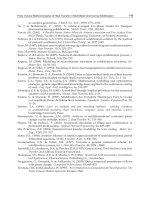
Figure 16 depicts the Nusselt number values versus 1
⁄
for purely electroosmotic flow. It
can be seen that to increase is to decrease Nusselt number. Increasing the Joule heating
effects results in more accumulation of energy near the wall and, consequently, higher wall
temperatures. The ultimate outcome thus will be smaller values of Nusselt number,
according to Eq. (106). As goes to infinity, for all values of , the Nusselt number
approaches 12 which is the classical solution for slug flow (Burmeister, 1993).
Fig. 16. Nusselt number versus 1
⁄
for purely electroosmotic flow
Unlike hydrodynamic features, the study of thermal features of electroosmosis is recent.
Maynes and Webb (2003) were the first who considered the thermal aspects of the
electroosmotic flow due to an external electric field. They analytically studied fully
developed electroosmotically generated convective transport for a parallel plate
microchannel and circular microtube under imposed constant wall heat flux and constant
wall temperature boundary conditions. Liechty et al. (2005) extended the above work to the
high zeta potentials. It was determined that elevated values of wall zeta potential produce
significant changes in the charge potential, electroosmotic flow field, temperature profile,
and Nusselt number relative to previous results invoking the Debye-Huckel linearization.
Also thermally developing electroosmotically generated flow in circular and rectangular
microchannels have been considered by Broderick et al. (2005) and Iverson et al. (2004),
respectively. The effect of viscous dissipation in fully developed electroosmotic heat transfer
for a parallel plate microchannel and circular microtube under imposed constant wall heat
flux and constant wall temperature boundary conditions was analyzed by Maynes and
Webb (2004). In a recent study, Sadeghi and Saidi (2010) derived analytical solutions for
thermal features of combined electroosmotically and pressure driven flow in a slit
microchannel, by taking into account the effects of viscous heating.
1/K
Nu
0 0.1 0.2 0.3 0.4 0.5
6
7
8
9
10
11
12
S=-1
S=0
S=1
S=2
Γ=0
Heat Transfer - Mathematical Modelling, Numerical Methods and Information Technology
524
3.3 Streaming potential
The EDL effects may be present even in the absence of an externally applied electric field.
Consider the pressure driven flow of an ionized liquid in a channel with negatively charged
surface. According to the Boltzmann distribution, there will be an excess of positive ions
over negative ions in liquid. The ultimate effect thus will be an electrical current due to the
liquid flow, called the streaming current,
. According to the definition of electrical current,
the streaming current is of the form
d
(110)
where is the channel cross sectional are and is the streamwise velocity. The streaming
current accumulates positive ions at the end of the channel. Consequently, a potential
difference, called the streaming potential, Φ
, is created between the two ends of the
channel. The streaming potential generates the so-called conduction current,
, which
carries charges and molecules in the opposite direction of the flow, creating extra impedance
to the flow motion. The net electrical current, , is the sum of the streaming current and the
conduction current and in steady state should be zero
0
(111)
In order to study the effects of the EDL on a pressure driven flow, first the conduction
current should be evaluated from Eqs. (110) and (111). Afterwards, the value of
is used to
find out the electric field associated with the flow induced potential,
, using the following
relationship
(112)
The flow induced electric field then is used to evaluate the body force in the momentum
equation. It should be pointed out that since there is not any electrical current due to an
external electric field, therefore, the Joule heating term does not appear in the energy
equation.
4. References
Arulanandam, S. & Li, D. (2000). Liquid transport in rectangular microchannels by
electroosmotic pumping. Colloids and Surfaces A: Physicochemical and Engineering
Aspects, Vol. 161, pp. 89–102, 0927-7757
Aydin, O. & Avci, M. (2006). Heat and flow characteristics of gases in micropipes, Int. J. Heat
Mass Transfer, Vol. 49, pp. 1723–1730, 0017-9310
Aydin, O. & Avci, M. (2007). Analysis of laminar heat transfer in micro-Poiseuille flow, Int. J.
Thermal Sciences, Vol.46, pp. 30–37, 1290-0729
Beskok, A. & Karniadakis, G.E. (1994). Simulation of heat and momentum transfer in complex
micro-geometries. J. Thermophysics Heat Transfer, Vol. 8, pp. 647–655, 0887-8722
Biswal, L.; Som, S.K. & Chakraborty, S. (2007). Effects of entrance region transport processes
on free convection slip flow in vertical microchannels with isothermally heated
walls. Int. J. Heat Mass Transfer, Vol. 50, pp. 1248–1254, 0017-9310
Heat Transfer at Microscale
525
Broderick, S.L.; Webb, B.W. & Maynes, D. (2005). Thermally developing electro-osmotic
convection in microchannels with finite Debye-layer thickness. Numerical Heat
Transfer, Part A, Vol. 48, pp. 941–964, 1040-7782
Burgreen, D. & Nakache, F.R. (1964). Electrokinetic flow in ultrafine capillary slits. J. Physical
Chemistry, Vol. 68, pp. 1084–1091, 1089-5639
Burmeister, L.C. (1993). Convective heat transfer, Wiley, 0471310204, New York
Chakraborty, S.; Som, S.K. & Rahul (2008). A boundary layer analysis for entrance region
heat transfer in vertical microchannels within the slip flow regime. Int. J. Heat Mass
Transfer, Vol. 51, pp. 3245–3250, 0017-9310
Chen, C.K. & Weng, H.C. (2005). Natural convection in a vertical microchannel. J. Heat
Transfer, Vol. 127, pp. 1053–1056, 0022-1481
Chen, C.H. (2009). Thermal transport characteristics of mixed pressure and electroosmotically
driven flow in micro- and nanochannels with Joule heating. J. Heat Transfer, Vol.
131, 022401, 0022-1481
Hadjiconstantinou, N.G. (2003). Dissipation in small scale gaseous flows. J. Heat Transfer,
Vol. 125, pp. 944-947, 0022-1481
Hadjiconstantinou, N.G. (2006). The limits of Navier Stokes theory and kinetic extensions for
describing small scale gaseous hydrodynamics. Phys. Fluids, Vol. 18, 111301, 1070-6631
Iverson, B.D.; Maynes, D. & Webb, B.W. (2004). Thermally developing electroosmotic
convection in rectangular microchannels with vanishing Debye-layer thickness. J.
Thermophysics Heat Transfer, Vol. 18, pp. 486–493, 0887-8722
Jeong, H.E. & Jeong, J.T. (2006a). Extended Graetz problem including axial conduction and
viscous dissipation in microtube, J. Mechanical Science Technology, Vol. 20, pp. 158–
166, 1976-3824
Jeong, H.E. & Jeong, J.T. (2006b). Extended Graetz problem including streamwise
conduction and viscous dissipation in microchannel, Int. J. Heat Mass Transfer, Vol.
49, pp. 2151–2157, 0017-9310
Kandlikar, S.G.; Garimella, S.; Li, D.; Colin, S. & King, M.R. (2006). Heat Transfer and Fluid
Flow in Minichannels and Microchannels, Elsevier, 0-0804-4527-6, Oxford
Kang, Y.; Yang, C. & Huang, X. (2002a). Dynamic aspects of electroosmotic flow in a
cylindrical microcapillary. Int. J. Engineering Science, Vol. 40, pp. 2203–2221, 0020-7225
Kang, Y.; Yang, C. & Huang, X. (2002b). Electroosmotic flow in a capillary annulus with
high zeta potentials. J. Colloid Interface Science, Vol. 253, pp. 285–294, 0021-9797
Karniadakis, G.; Beskok, A. & Aluru, N. (2005). Microflows and Nanoflows, Fundamentals and
Simulation, Springer, 0-387-90819-6, New York
Kennard, E.H. (1938). Kinetic Theory of Gases, McGraw–Hill, New York
Koo, J. & Kleinstreuer, C. (2003). Liquid flow in microchannels: experimental observations
and computational analyses of microfluidics effects. J. Micromechanics and
Microengineering, Vol. 13, pp. 568–579, 1361-6439
Koo, J. & Kleinstreuer, C. (2004). Viscous dissipation effects in microtubes and
microchannels, Int. J. Heat Mass Transfer, Vol. 47, pp. 3159–3169, 0017-9310
Levine, S.; Marriott, J.R.; Neale, G. & Epstein, N. (1975). Theory of electrokinetic flow in fine
cylindrical capillaries at high zeta-potentials. J. Colloid Interface Science, Vol. 52, 136–
149, 0021-9797
Liechty, B.C.; Webb, B.W. & Maynes, R.D. (2005). Convective heat transfer characteristics of
electro-osmotically generated flow in microtubes at high wall potential. Int. J. Heat
Mass Transfer, Vol. 48, pp. 2360–2371, 0017-9310
Heat Transfer - Mathematical Modelling, Numerical Methods and Information Technology
526
Masliyah J.H. & Bhattacharjee, S. (2006). Electrokinetic and Colloid Transport Phenomena, First
ed., John Wiley, 0-471-78882-1, New Jersey.
Maxwell, J.C. (1879). On stresses in rarefied gases arising from inequalities of temperature,
Philos. Trans. Royal Soc., Vol. 170, pp. 231-256
Maynes, D. & Webb, B.W. (2003). Fully developed electroosmotic heat transfer in
microchannels. Int. J. Heat Mass Transfer, Vol. 46, pp. 1359–1369, 0017-9310
Maynes, D. & Webb, B.W. (2004). The effect of viscous dissipation in thermally fully
developed electroosmotic heat transfer in microchannels. Int. J. Heat Mass Transfer,
Vol. 47, pp. 987–999, 0017-9310
Niazmand, H.; Jaghargh, A.A. & Renksizbulut, M. (2010). Slip-flow and heat transfer in
isoflux rectangular microchannels with thermal creep effects. J. Applied Fluid
Mechanics, Vol. 3, pp. 33-41, 1735-3645
Ou, J.W. & Cheng, K.C. (1973). Effects of flow work and viscous dissipation on Graetz
problem for gas flows in parallel-plate channels, Heat Mass Transfer, Vol. 6, pp. 191–
198, 0947-7411
Probstein, R.F. (1994). Physicochemical Hydrodynamics, 2nd ed. Wiley, 0471010111, New York
Rice, C.L. & Whitehead, R. (1965). Electrokinetic flow in a narrow cylindrical capillary. J.
Physical Chemistry, Vol. 69, pp. 4017–4024, 1089-5639
Rij, J.V.; Harman, T. & Ameel, T. (2007). The effect of creep flow on two-dimensional isoflux
microchannels. Int. J. Thermal Sciences, Vol. 46, pp. 1095–1103, 1290-0729
Rij, J.V.; Ameel, T. & Harman, T. (2009). The effect of viscous dissipation and rarefaction on
rectangular microchannel convective heat transfer. Int. J. Thermal Sciences, Vol. 48,
pp. 271–281, 1290-0729
Sadeghi, A.; Asgarshamsi, A. & Saidi M.H. (2009). Analysis of laminar flow in the entrance
region of parallel plate microchannels for slip flow, Proceedings of the Seventh
International ASME Conference on Nanochannels, Microchannels and Minichannels,
ICNMM2009, S.G. Kandlikar (Ed.), Pohang, South Korea
Sadeghi, A. & Saidi, M.H. (2010). Viscous dissipation and rarefaction effects on laminar
forced convection in microchannels. J. Heat Transfer, Vol. 132, 072401, 0022-1481
Sadeghi, A. & Saidi, M.H. (2010). Viscous dissipation effects on thermal transport
characteristics of combined pressure and electroosmotically driven flow in
microchannels. Int. J. Heat Mass Transfer, Vol. 53, pp. 3782–3791, 0017-9310
Taheri, P.; Torrilhon, M. & Struchtrup, H. (2009). Couette and Poiseuille microflows:
analytical solutions for regularized 13-moment equations. Phys. Fluids, Vol. 21,
017102, 1070-6631
Tunc, G.& Bayazitoglu, Y. (2002). Heat transfer in rectangular microchannels. Int. J. Heat
Mass Transfer, Vol. 45, pp. 765–773, 0017-9310
Weng, H.C. & Chen, C.K. (2008a). On the importance of thermal creep in natural convective
gas microflow with wall heat fluxes. J. Phys. D, Vol. 41, 115501, 0022-3727
Weng, H.C. & Chen, C.K. (2008b). Variable physical properties in natural convective gas
microflow. J. Heat Transfer, Vol. 130, 082401, 0022-1481
Yang, C.; Li, D. & Masliyah, J.H. (1998). Modeling forced liquid convection in rectangular
microchannels with electrokinetic effects. Int. J. Heat Mass Transfer
, Vol. 41, pp.
4229–4249, 0017-9310
Yu, S. & Ameel, T.A. (2001). Slip flow heat transfer in rectangular microchannels. Int. J. Heat
Mass Transfer, Vol. 44, pp. 4225–4234, 0017-9310
Part 4
Energy Transfer and Solid Materials
21
Thermal Characterization of Solid Structures
during Forced Convection Heating
Balázs Illés and Gábor Harsányi
Department of Electronics Technology,
Budapest University of Technology and Economic
Hungary
1. Introduction
By now the forced convection heating became an important part of our every day life. The
success could be thanked to the well controllability, the fast response and the efficient heat
transfer of this heating technology. We can meet a lot of different types of forced convection
heating methods and equipments in the industry (such as convection soldering oven,
convection thermal annealing, paint drying, etc.) and also in our household (such as air
conditioning systems, convection fryers, hair dryers, etc.).
In every cases the aim of the mentioned applications are to heat or cool some kind of solid
materials and structures. If we would like to examine this heating or cooling process with
modeling and simulation, first we need to know the physical parameters of the forced
convection heating such as the velocity, the pressure and the density space of the flow,
together with the temperature distribution and the heat transfer coefficients on the different
points of the heated structure. Therefore in this chapter, first we present the mathematical
and physical basics of the fluid flow and the convection heating which are needed to the
modeling and simulation. We show some models of gas flows trough typical examples in
aspect of the heat transfer. We discuss the theory of free-streams, the vertical – radial
transformation of gas flows and the radial gas flow layer formation on a plate. The models
illustrate how we can study the velocity, pressure and density space in a fluid flow and we
also point how these parameters effect on the heat transfer coefficient.
After it new types of measuring instrumentations and methods are presented to characterize
the temperature distribution in a fluid flow. Calculation methods are also discussed which
can determine the heat transfer coefficients according to the dynamic change of the
temperature distribution. The ability of the measurements and calculations will be
illustrated with two examples. In the first case we determine the heat transfer coefficient
distribution under free gas streams. The change of the heat transfer coefficient is examined
when the heated surface shoves out the gas stream. In the second case we study the
direction characteristics of the heat transfer coefficient in the case of radial flow layers on a
plate in function of the height above the plate. It is also studied how the blocking elements
towards the flow direction affects on the formation of the radial flow layer.
In the last part of our chapter we present how the measured and calculated heat transfer
coefficients can be applied during the thermal characterization of solid structures. The
mathematical and physical description of a 3D thermal model is discussed. The model based
Heat Transfer - Mathematical Modelling, Numerical Methods and Information Technology
530
on the thermal (central) node theory and the calculations based on the Finite Difference
Method (FDM). We present a new cell partition method, the Adaptive Interpolation and
Decimation (AID) which can increase the resolution and the accuracy of the model in the
investigated areas without increasing the model complexity. With the collective application
of the thermal cell method, the FDM calculations and the AID cell partition, the model
description is general and the calculation time of the thermal model is very short compared
with the similar Finite Element Method (FEM) models.
2. Basics of convection heating and fluid flow
The phrase of “Convection” means the movement of molecules within fluids (i.e. liquids,
gases and rheids). Convection is one of the major modes of heat transfer and mass transfer.
Convective heat and mass transfer take place through both diffusion – the random
Brownian motion of individual particles in the fluid – and by advection, in which matter or
heat is transported by the larger-scale motion of currents in the fluid. In the context of heat
and mass transfer, the term "convection" is used to refer to the sum of advective and
diffusive transfer (Incropera & De Witt, 1990). There are two major types of heat convection:
1. Heat is carried passively by a fluid motion which would occur anyway without the
heating process. This heat transfer process is often termed forced convection or
occasionally heat advection.
2. Heat itself causes the fluid motion (via expansion and buoyancy force), while at the
same time also causing heat to be transported by this bulk motion of the fluid. This
process is called natural convection, or free convection.
Both forced and natural types of heat convection may occur together (in that case being
termed mixed convection). Convective heat transfer can be contrasted with conductive heat
transfer, which is the transfer of energy by vibrations at a molecular level through a solid or
fluid, and radiative heat transfer, the transfer of energy through electromagnetic waves.
2.1 The convection heating
Convection heating is usually defined as a heat transfer process between a solid structure
and a fluid (in the following we will use this type of interpretation). The performance of the
convection heating mainly depends on the heat transfer coefficient and can be characterized
by the convection heat flow rate from the heater fluid to the heated solid material (Newton’s
law) (Castell et al., 2008; Gao et al., 2003):
(()-())
c
cht
dQ
FhATtTt
dt
==⋅⋅
[w] (1)
where A is the heated area [m
2
], T
h
(t) is the temperature of the fluid [K], T
t
(t) is the
temperature of the solid material [K] and h is the heat transfer coefficient [W/m
2
K] on the A
area.
The heat transfer coefficient can be defined as some kind of “concentrated parameter” which
is characterised by the density and the velocity filed of the fluid used for heating, the angle
of incidence between the solid structure and the fluid, and finally the roughness of the
heated surface (Kays et al., 2004). The value of the heat transfer coefficient can vary between
wide ranges but it is typically between 5 and 500 [W/mK] in the case of gases. In a lot of
application the material of the fluid and the roughness of the heated surface can be consider
Thermal Characterization of Solid Structures during Forced Convection Heating
531
to be constant. Therefore mainly the gas flow parameters (density and velocity) influence
the heat transfer coefficient which can be characterized by the mass flow rate q
m
(Tamás,
2004):
m
A
qvdA
ρ
=
⋅⋅
∫
[kg/s] (2)
where ρ is the density of the fluid [kg/m
3
], v is the velocity of the fluid [m/s] and A is the
are whereon q
m
is defined.
As you can see in Eq. (1) the calculation of the convection heat transfer is very simple if we
know the exact value of the heat transfer coefficient. The problem is that in most of the cases
this value is not known. Although we know the influence parameters (velocity, density, etc.)
on the heat transfer coefficient but the strength of dependence from the different parameters
changes in every cases. There are not existed explicit formulas to determine the heat transfer
coefficient only in some special cases.
Inoue (Inoue & Koyanagawa, 2005) has approximated the h parameter of the heater gas
streams from the nozzle-matrix blower system with the followings:
()() ()()
(
)
()() ()()
0.05
6
22
2
0.42
3
22
/4 / 1 2.2 /4 /
/
Re Pr 1
1 0.2( / 6) / 4 / 0.6 / / 4 /
Dl Dl
Hd
h
d
HD Dl Dl
ππ
λ
ππ
−
−
=+
+−
⎡⎤
⎛⎞
⎢⎥
⎜⎟
⎢⎥
⎜⎟
⎢⎥
⎝⎠
⎣⎦
(3)
where λ is thermal conductivity of the gas [W/m.K], d is the diameter of the nozzles, H is the
distance between nozzles and the target [m], r is the distance between the nozzles in the
matrix [m], Re is the Reynolds number and Pr is the Prandtl number. The Eq. (3) shown
above, has been derived from systematic series of experiments. But unfortunately this
method only gives an average value of h and can not deal with the changes of the blower
system (contamination, aging, etc.). In addition in many cases it is difficult to determine the
exact value of some parameters e.g. the velocity and density of the gas which are needed for
Re and Pr numbers.
The same problem occurs in case of other approximations e.g. Dittus–Boelter, Croft–Tebby,
Soyars, etc. (a survey of these methods can be seen in (Guptaa et al, 2009)). The simplest way
to approximate h is carried out with the linear combination of the velocity and some
constants (Blocken et al., 2009), but it gives useful results only in case of big dimensions (e.g.
buildings). Other methods calculate h from the mass flow (Bilen et al., 2009; Yin & Zhang,
2008; Dalkilic et al., 2009), but in this case determining the mass flow is also as difficult as
determining the velocity.
Therefore in most of the cases the easiest way to determine the heat transfer coefficient is the
measuring (see details in Section 4), however it is also important that we can study the effect
of the environmental circumstances on the h parameter with gas flow models (see details in
Section 3).
2.2. Basics of fluid dynamics
The main issue of this topic is the forced convection when the heat is transported by forced
movement of a fluid. Therefore the fluid dynamics are important tools during the study of
various forced convection heating methods. During the description of fluid movements,
Newton 2
nd
axiom can be applied, which creates relation between the acting forces on the
Heat Transfer - Mathematical Modelling, Numerical Methods and Information Technology
532
fluid particles and the change of the momentum of the fluid particles. Take an elementary
fluid particle which moves in the flowing space (Fig. 1.a).
Fig. 1. a) Elementary fluid particle in the flowing phase; b) elementary fluid particle in the
flowing phase (natural coordinate system); c) acting stresses towards the x direction.
The acting forces are originated from two different sources:
- forces acting on the mass of the fluid particles (e.g. gravity force),
- forces acting on the surface of the fluid particles (e.g. pressure force).
According to these the most common momentum equation – when the friction is neglected
and the flow is stationer – is the Euler equation (Tamás, 2004):
1dv
vggradp
dr
ρ
=−
(4)
where v is the velocity of the fluid [m/s], t is the time [s], g is the gravity force, ρ is the
density [kg/m
3
] and p is the pressure. Another important form of this equation – which is
often used in the case of the vertical–radial transformation of fluid flows (see in Section 3.) –
is defined in natural coordinate system (Fig. 1.b). The natural coordinate system is fixed to
the streamline. The connection point is G1. The tangential (e) and the normal (n) coordinate
axis are in one plan with the velocity vector (v). In the ambiance of G1 the streamline can be
supplemented by an arc which has R radius and G2 center. In this natural coordinate system
the Euler equation (vector form) is the following (Tamás, 2004):
1
e
v
p
vg
ee
ρ
∂
∂
=−
∂
∂
and
2
1
n
v
p
g
Rn
ρ
∂
−=−
∂
and
1
0
b
p
g
b
ρ
∂
=−
∂
(5)
In the previous equations we have neglected the effect of friction. However in a lot of
convection heating examples this is a non-accurate approach. In the area where the moving
fluid touches a solid material the effect of friction can be considerable both form the point of
the flowing and the heating. The effect of friction can be determined as some kind of force
acting on the surfaces of the moving fluid particle such as the pressure. In Fig. 1.c the
stresses acting towards the x direction is presented.
The sheer stresses (τ) [Pa] and the tensile stresses (σ) [Pa] usually changes in space and this
changes cause the accelerating force on the fluid particle. The stress tensor is:
Thermal Characterization of Solid Structures during Forced Convection Heating
533
xyxzx
xy y zy
xz yz z
στ τ
τστ
ττσ
Φ=
⎡
⎤
⎢
⎥
⎢
⎥
⎢
⎥
⎣
⎦
(6.1)
In most of the cases the tensile stresses are caused by only the pressure, therefore:
p
σ
=
−
(6.2)
and the sheer stresses can be defined according to the Newton’s viscosity law:
y
x
yx
v
v
x
y
τμ
∂
∂
=+
∂∂
⎛⎞
⎜⎟
⎝⎠
(6.3)
where μ is the viscosity of the fluid [kg/m.s]. So
y
x
τ
means the tensile stress towards the x
direction on the plane with y normal. The other tensile stresses can be defined by the similar
way. With the application of the stress tensor the momentum equation can be expressed (the
flow is still stationer):
1dv
vg
dr
ρ
=
+Φ∇ (7)
where
∇ is the nabla vector. The vector form of the momentum equation is more interesting
and more often used which is:
2
222
22
1
y
xxx x zx
xyz x
v
vvv v vv
p
vvvg
x
y
zx
y
xzx
xx
μμ
ρ
∂
∂∂∂ ∂ ∂∂
∂
+ + =+ −+ + + +
∂∂∂ ∂ ∂∂ ∂∂
∂∂
⎛⎞
⎛⎞
⎛⎞
⎜⎟
⎜⎟
⎜⎟
⎜⎟
⎜⎟
⎝⎠
⎝⎠
⎝⎠
(8.1)
22
22
22
1
yyy y y
xz
xyz y
vvv v v
vv
p
vvvg
x
y
zx
yy
z
y
yy
μμ
ρ
∂∂∂ ∂ ∂
∂∂
∂
++=+ +−++ +
∂∂∂ ∂∂∂ ∂∂
∂∂
⎛⎞
⎛⎞⎛⎞
⎜⎟
⎜⎟⎜⎟
⎜⎟⎜⎟
⎜⎟
⎝⎠⎝⎠
⎝⎠
(8.2)
2
22 2
22
1
y
zzz xz z
xyz z
v
vvv vv v
p
vvvg
x
y
zxz
y
zz
zz
μμ
ρ
∂
∂∂∂ ∂∂ ∂
∂
++=+ ++ +−
∂∂∂ ∂∂ ∂∂∂
∂∂
⎛⎞
⎛⎞
⎛⎞
⎜⎟
⎜⎟
⎜⎟
⎜⎟
⎜⎟
⎝⎠
⎝⎠
⎝⎠
(8.3)
3. Application examples of convection heating
In the followings we concentrate only for forced convection heating methods which apply
some kind of gas flows. The gas flows can be usually considered to be laminar; therefore the
analysis of them is much easier than other fluid flows where this condition is not existed. In
this Section typical convection heating applications is studied from the point of gas flow.
Simple gas flow models are presented to examine how the changes of the flow parameters
effect on the value of the heat transfer coefficient.
The most common and widely used example for the convection heating is the heating with
concentrated gas streams. The gas streams blow trough nozzles with d
0
diameter into a free
space where the heat structure is placed. Before the deeper analysis, we will discus the basic
of this technology which is the free-stream theory.