Heat Transfer Mathematical Modelling Numerical Methods and Information Technology Part 17 pot

Thermal Aspects of Solar Air Collector

629
[2] Rene Tchinda, A review of the mathematical models for predicting solar air heaters
systems, Renewable and Sustainable Energy Reviews 13 (2009) 1734–1759.
[3] Perrot, Pierre, A to Z of Thermodynamics, Oxford University Press, Oxford, 1998.
[4] Rant, Z., Exergy, a new word for technical available work, Forschung auf dem Gebiete
des Ingenieurwesens 22, (1956), pp. 36–37.
[5] Gibbs, J. W. ,A method of geometrical representation of thermodynamic properties of
substances by means of surfaces: reprinted in Gibbs, Collected Works, ed. W. R.
Longley and R. G. Van Name, Transactions of the Connecticut Academy of Arts
and Sciences, 2, (1931), pp. 382–404 .
[6] Moran, M. J. and Shapiro, H. N., Fundamentals of Engineering Thermodynamics, 6th
Edition, 2007.
[7] Van Wylen, G.J., Thermodynamics, Wiley, New York, 1991.
[8] Wark, J. K., Advanced Thermodynamics for Engineers, McGraw-Hill, New York, 1995.
[9] Bejan, A., Advanced Engineering Thermodynamics, 2nd Edition, Wiley, 1997.
[10] Saravan , M. Saravan, R and Renganarayanan, S. , Energy and Exergy Analysis of
Counter flow Wet Cooling Towers, Thermal Science, 12, (2008), 2, pp. 69-78.
[11] Bejan, A., Kearney, D. W., and Kreith, F., Second Law Analysis and Synthesis of Solar
Collector Systems, Journal of Solar Energy Engineering, 103, (1981), pp. 23-28.
[12] Bejan, A. , Entropy Generation Minimization, New York, CRC press, 1996.
[13] Londono-Hurtado, A. and Rivera-Alvarez, A., Maximization of Exergy Output From
Volumetric Absorption Solar Collectors, Journal of Solar Energy Engineering , 125,
(2003) ,1 , pp. 83-86.
[14] Luminosu, I and Fara, L., Thermodynamic analysis of an air solar collector,
International Journal of Exergy, 2, (2005), 4, pp. 385-408.
[15] Altfeld, K,. Leiner, W., Fiebig, M., Second law optimization of flat-plate solar air
heaters Part I: The concept of net exergy flow and the modeling of solar air heaters,
Solar Energy 41, (1988), 2, pp. 127-132.
[16] Altfeld, K., Leiner, W., Fiebig, M., Second law optimization of flat-plate solar air

heaters Part 2: Results of optimization and analysis of sensibility to variations of
operating conditions, Solar Energy, 41, (1988),4 , pp. 309-317.
[17] Torres-Reyes, E., Navarrete-Gonzàlez, J. J., Zaleta-Aguilar, A., Cervantes-de Gortari, J.
G., Optimal process of solar to thermal energy conversion and design of
irreversible flat-plate solar collectors, Energy 28, (2003), pp. 99–113.
[18] Kurtbas, I., Durmuş, A., Efficiency and exergy analysis of a new solar air heater,
Renewable Energy, 29, (2004), pp. 1489-1501.
[19] Choudhury C, Chauhan PM, Garg HP. Design curves for conventional solar air heaters.
Renewable energy 1995;6(7):739–49.
[20] Ong KS. Thermal performance of solar air heaters: mathematical model and solution
procedure. Solar Energy 1995;55(2):93–109.
[21] Hegazy AA. Thermohydraulic performance of heating solar collectors with variable
width, flat absorber plates. Energy Conversion and Management 2000;41:1361–78.
[22] Al-Kamil MT, Al-Ghareeb AA. Effect of thermal radiation inside solar air heaters.
Energy Conversion and Management 1997;38(14):1451–8.
[23] Garg HP, Datta G, Bhargava K. Some studies on the flow passage dimension for solar
air testing collector. Energy Conversion and Management 1984;24(3):181–4.
Heat Transfer - Mathematical Modelling, Numerical Methods and Information Technology

630
[24] Forson FK, Nazha MAA, et Rajakaruna H. Experimental and simulation studies on a
single pass, double duct solar air heater. Energy Conversion and Management
2003;44:1209–27.
[25] Ho CD, Yeh HM, Wang RC. Heat-transfer enhancement in double-pass flatplate solar
air heaters with recycle. Energy 2005;30:2796–817.
[26] Duffie J.A, Beckman W.A, Solar engineering of thermal processes, 2nd ed. New York,
John Wiley, 1991.
27
Heat Transfer in Porous Media
Ehsan Mohseni Languri

1
and Davood Domairry Ganji
2

1
University of Wisconsin - Milwaukee
2
Noshirvani Technical University of Babol,
1
USA
2
Iran
1. Introduction
Heat transfer phenomena play a vital role in many problems which deals with transport of
flow through a porous medium. One of the main applications of study the heat transport
equations exist in the manufacturing process of polymer composites [1] such as liquid
composite molding. In such technologies, the composites are created by impregnation of a
preform with resin injected into the mold’s inlet. Some thermoset resins may undergo the
cross-linking polymerization, called curing reaction, during and after the mold-filling stage.
Thus, the heat transfer and exothermal polymerization reaction of resin may not be
neglected in the mold-filling modeling of LCM. This shows the importance of heat transfer
equations in the non-isothermal flow in porous media.
Generally, the energy balance equations can be derived using two different approaches: (1)
two-phase or thermal non-equilibrium model [2-6] and (2) local thermal equilibrium model
[7-18]. There are two different energy balance equations for two phases (such as resin and
fiber in liquid composite molding process) separately in the two-phase model, and the heat
transfer between these two equations occur via the heat transfer coefficient. In the thermal
equilibrium model, we assume that the phases (such as resin and fiber) reach local
thermodynamic equilibrium. Therefore, only one energy equation is needed as the thermal
governing equation, [3,5]. Firstly, we consider the heat transfer governing equation for the

simple situation of isotropic porous media. Assume that radioactive effects, viscous
dissipation, and the work done by pressure are negligible. We do further simplification by
assuming the thermal local equilibrium that
sf
TT T
=
= where
s
T
and
f
T are the solid and
fluid phase temperature, respectively. A further assumption is that there is a parallel
conduction heat transfer taking place in solid and fluid phases.
Taking the average over an REV of the porous medium, we have the following for solid and
fluid phases,

(1 )( ) (1 ) .( ) (1 )
s
s
s
ssss
T
ckTq
t
ϕρ ϕ ϕ
∂< >
′
′′
−=−∇∇<>+−

∂
(1)

() (). .( )
f
f
ff
P
f
P
ff ff f
T
ccvTkTq
t
ϕ
ρρϕϕ
∂< >
′
′′
+∇<>=∇∇<>+
∂
(2)
Heat Transfer - Mathematical Modelling, Numerical Methods and Information Technology

632
where
c is the specific heat of the solid and
p
c is the specific heat at constant pressure of the
fluid,

k is the thermal conductivity coefficient and q
′
′′
is the heat production per unit
volume. By assuming the thermal local equilibrium, setting
sf
TT T
=
= , one can add Eqs. (1)
and (2) to have:

() ()
()
mm
mf
T
ccvTkTq
t
ρρ
∂< >
′
′′
+∇<>=∇∇<>+
∂
(3)
where
()
m
c
ρ

,
m
k and
m
q
′
′′
are the overall heat capacity, overall thermal conductivity, and
overall heat conduction per unit volume of the porous medium, respectively. They are
defined as follows:

() (1 )() ( )
ms
pf
ccc
ρ
ϕρ ϕρ
=
−+ (4)

(1 )
ms
f
kkk
ϕ
ϕ
=
−+ (5)
(1 )
ms

f
qqq
ϕ
ϕ
′
′′ ′′′ ′′′
=
−+ (6)
2. Governing equations
2.1 Macroscopic level
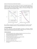
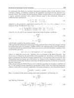
Pillai and Munagavalasa [19] have used volume averaging method with the local thermal
equilibrium assumption to derive a set of energy and species equations for dual-scale porous
medium. The schematic view of such volume is presented in the figure 1. Unlike the single
scale porous media, there is an unsaturated region behind the moving flow-front in the dual-
scale porous media. The reason for such partially saturated flow-front can be mentioned as
the flow resistance difference between the gap and the tows where the flow goes faster in the
gaps rather than the wicking inside the tows. Pillai and Munagavalasa [19] have applied the
volume averaging method to the dual-scale porous media. Using woven fiber mat in the LCM,
they considered the fiber tows and surrounding gaps as the two phases.

Fig. 1. Schematic view of dual-scale porous-medium [19]
Heat Transfer in Porous Media

633
The pointwise microscopic energy balance and species equations for resin inside the gap
studied at first, and then the volume average of these equation is taken. Finally, they came
up with the macroscopic energy balance and species equations.
The macroscopic energy balance equation in dual-scale porous medium is given by

,

K.
gg g
g
P
gg g g g
th
ggg
R c conv cond
CTvT THfQQ
t
ρε ερ
∂
⎡⎤
+∇ =∇∇ + + −
⎢⎥
∂
⎣⎦
(7)
where the
g
ρ
and
,P
g
C are the resin density and specific heat respectively.
g
T is the
temperature of resin in the gap region,
g
ε

is gap fraction,
R
H is the heat reaction and
c
f
is
the reaction rate. The
gg
Rc
H
f
ε
ρ
term represents the heat source due to exothermic curing
reaction. The term
th
K is the thermal conductivity tensor for dual-scale porous medium
defined as

,
ˆ
VV
gt
ggPgg
th g g gt g
g
A
kC
K k n bdA v bdV
ρε

εδ
=+ −
∫∫
(8)
where
g
k
, δ and
ˆ
g
v
are thermal conductivity of the resin, a unit tensor and the fluctuations
in the gap velocity with respect to the gap averaged velocity respectively. The vector b
relates temperature deviations in the gap region to the gradient of gap-averaged
temperature in a closure. Considering the temperature closure formulation as
ˆ
.
g
gg
Tb T=∇< >
, the local temperature deviation is related to the gradient of the gap-
averaged temperature through the vector b , [19].
conv
Q
in the Eq. (8) is the heat source term due to release of resin heat prior to the absorption
of surrounding tows given by

,
[]
gg

t
conv g P g g g g
QCSTT
ρ
=− (9)
where Sg , the sink term and areal average of temperature on the tow-gap interface are
expressed as following respectively

1
.
gggt
g
SvndA
V
ε
=
∫
(10)
and

1
gt
gg
gt
TTdA
A
=
∫
(11)
and

cond
Q is the heat sink term caused by conductive heat loss to the tows given by

1
().
cond g g gt
QkTndA
V
=−∇
∫
(12)
Using the analogy between heat and mass transfer to derive the gap-averaged cure
governing equation following the Tucker and Dessenberger [6] approach, one can derive the
following equation
Heat Transfer - Mathematical Modelling, Numerical Methods and Information Technology

634

ggg
gg g g g g
cconvdi
ff
cvc Dc fMM
t
εε
∂
+∇ =∇∇ ++ −
∂
(13)
where

g
c is the degree of cure in a resin which value of 0 and 1 correspond to the uncured
and fully cured resin situation,
D is diffusivity tensor for the gap flows and is given by

1
1
ˆ
dV
V
g
ggt g
g
D
DD nbd vb
ε
εδ
=+ −
∫∫
A
V
(14)
where
1
D is the molecular diffusivity of resin. In the Eq. (13),
conv
M is the convective source
due to release of resin cure when absorbing into tows as a results of sink effect, given by

MS[ ]

gg
t
conv g g g
cc=−
(15)
where
g
t
g
c is the areal average of temperature on the tow-gap interface, expressed as

1
gt
gt
gg
gt
A
ccdA
A
=
∫
(16)
and
di
ff
M is the cure sink term as a result of the diffusion of cured resin into the tows, given by

1
1
().

diff g gt
M
DcndA
V
=−∇
∫
(17)
It should be noted that the only way to compute the
conv
Q ,
cond
Q ,
conv
M and
di
ff
M is solving
for flow and transport inside the tows.
2.2 Microscopic level
Phelan et al. [20] showed that the conventional volume averaging method can be directly
used to derive the transport equation for thermo-chemical phenomena inside the tows for
single-scale porous media. The final derivation for microscopic energy equation is

()
()
() ()
,
[1 ]
t
t

p
tP Ptt thtttlRc
fl
l
T
CCCvTKTHf
t
ερ ε ρ ρ ερ
∂
+− + ∇=∇ ∇+
∂
(18)
where the subscript
t refer to tows. The microscopic species equation is given by


t
tttttttc
c
vc Dc f
t
ε
εε
∂
+∇=∇ ∇+
∂
(19)
The complete set of microscopic and macroscopic energy and species equations as well as the
flow equation should be solved to model the unsaturated flow in a dual-scale porous medium.
3. Dispersion term

In some cases, a further complication arises in the thermal governing equation due to
thermal dispersion [21]. The thermal dispersion happens due to hydrodynamic mixing of
fluid at the pore scale. The mixings are mainly due to molecular diffusion of heat as well as
Heat Transfer in Porous Media

635
the mixing caused by the nature of the porous medium. The mixings are mainly due to
molecular diffusion of heat as well as the mixing caused by the nature of the porous
medium. Greenkorn [22] mentioned the following nine mechanisms for most of the mixing;
1.
Molecular diffusion: in the case of sufficiently long time scales
2.
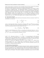
Mixing due to obstructions: The flow channels in porous medium are tortuous means
that fluid elements starting a given distance from each other and proceeding at the
same velocity will not remain the same distance apart, Fig. 2.
3.
Existence of autocorrelation in flow paths: Knowing all pores in the porous medium are
not accessible to the fluid after it has entered a particular fluid path.
4.
Recirculation due to local regions of reduced pressure: The conversion of pressure
energy into kinetic energy gives a local region of low pressure.
5.
Macroscopic or megascopic dispersion: Due to nonidealities which change gross
streamlines.
6.
Hydrodynamic dispersion: Macroscopic dispersion is produced in capillary even in the
absence of molecular diffusion because of the velocity profile produced by the adhering
of the fluid wall.
7.
Eddies: Turbulent flow in the individual flow channels cause the mixing as a result of

eddy migration.
8.
Dead-end pores: Dean-end pore volumes cause mixing in unsteady flow. The main
reason is as solute rich front passes the pore, diffusion into the pore occurs due to
molecular diffusion. After the front passes, the solute will diffuse back out and thus,
dispersing.
9.
Adsorption: It is an unsteady-state phenomenon where a concentration front will
deposit or remove material and therefore tends to flatten concentration profiles.


Fig. 2. Mixing as a result of obstruction
Heat Transfer - Mathematical Modelling, Numerical Methods and Information Technology

636
Rubin [23] generalized the thermal governing equation

() ()
()
mm
mf
T
ccvTkTq
t
ρρ
∂
′
′′
+∇=∇∇+
∂

(20)
where
K is a second-order tensor called dispersion tensor.
Two dispersion phenomena have been extensively studied in the transport phenomena in
porous media are the mass and thermal dispersions. The former involves the mass of a
solute transported in a porous medium, while the latter involves the thermal energy
transported in the porous medium. Due to the similarity of mass and thermal dispersions,
they can be described using the dimensionless transport equations as

1
iij
iij
UD
XPeX X
θ
⎛⎞
∂
Ω∂Ω ∂Ω
∂
⎜⎟
+=
⎜⎟
∂∂∂∂
⎝⎠
(21)
where
Ω is either averaged concentration for mass dispersion or averaged dimensionless
temperature for thermal dispersion, θ is dimensionless time,
i
U is averaged velocity

vector, Pe is Peclet number, D
ij
is dispersion tensor of 2
nd
order. It should be noted that
uL
Pe =
D
in mass dispersion and
uL
Pe
α
=
in thermal dispersion where u and L are
characteristic velocity and length, respectively.
D
and α are molecular mass and thermal
diffusivities, respectively.
3.1 Dispersion in porous media
Most studies on dispersion tensor so far have been focusing on the isotropic porous media.
Nikolaveskii [24] obtained the form of dispersion tensor for isotropic porous media by
analogy to the statistical theory of turbulence. Bear [25] obtained a similar result for the form
of the dispersion tensor on the basis of geometrical arguments about the motion of marked
particles through a porous medium. Bear studied the relationship between the dispersive
property of the porous media as defined by a constant of dispersion, the displacement due
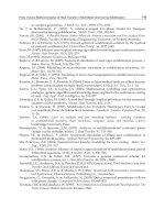
to a uniform field of flow, and the resulting distribution. He used a point injection subjected
to a sequence of movements. The volume averaged concentration of the injected tracer,
0
C ,
around a point which is displaced a distance Lut

=
in the direction of the uniform, isotropic,
two dimensional field of flow from its original position is considered in his research.

22
0
00
22 2 2
xy x y
C
mn
(x,y;x ,y ) .exp
2πσ σ 2σ 2σ
C
⎧
⎫
⎪
⎪
=−−
⎨
⎬
⎪
⎪
⎩⎭
(22)
where L is the distance of mean displacement,
u is the uniform velocity of flow, t is the time
of flow,
x
σ

and
y
σ
are standard deviations of the distribution in the x and y directions,
respectively and, finally m and n are the coordinates of the point (x,y) in the coordinate
system centered at
(
)
,
ξ
η
given by
0
mx(x L)
=
−+
and
0
n
yy
=
−
, figure 3. This figure
shows a point injection as a result of subsequence movement where initially circle tracer
gets an elliptic shape at L ut
=
.
Heat Transfer in Porous Media

637

Fig. 3. Dispersion of a point injection displaced a distance L
Standard deviations are defined by
()
0.5
xI
σ 2D L= and
()
0.5
yII
σ 2D L= where
I
D and
II
D
are the longitudinal and transverse constants of dispersion in porous media, respectively.
One should note that the
I
D and
II
D used in the Bear work depend only upon properties of
the porous medium such as porosity, grain size, uniformity, and shape of grains. From Eq.
(22), it follows that, after a uniform flow period, lines of the similar concentration resulting
from the circular point injection of the tracer take the ellipse shape centered at the displaces
mean point and oriented with their major axes in the direction of the flow.

2
2
22
1

xy
y
x
σσ
+
= (23)
Bear conjectured that the property which is defined by the constant of dispersion,
i
j
kl
D ,
depends only upon the characteristics of porous medium and the geometry of its pore-
channel system. In a general case, this is a fourth rank tensor which contains 81 components.
These characteristics are expressed by the longitudinal and lateral constants of dispersion of
the porous media. Scheidegger [26] used the dispersion tensor
D
ij
in the following form

km
ij ijkm
vv
Da
v
= (24)
where
v is the average velocity vector, v
k
is the
th

k component of velocity vector, a
ijkm
is a
fourth rank tensor called geometrical dispersivity tensor of the porous medium. Bear
demonstrated how the dispersion tensor relates to the two constants for an isotropic
medium:
||
a = longitudinal dispersion
1
, and a
⊥
= transversal dispersion
2
. Scheidegger [26]
has shown that there are two symmetry properties for dispersivity tensor

1
The longitudinal direction is along the mean flow velocity in porous media, whereas the transverse
direction is perpendicular to the mean flow velocity.

Heat Transfer - Mathematical Modelling, Numerical Methods and Information Technology

638

i
j
km
j
ikm
aa

=
and
i
j
km i
j
mk
aa
=
(25)
Therefore, only 36 of 81 components of fourth rank tensor
a
ijkl
is independent. For an
isotropic porous medium, the dispersivity tensor must be isotropic. An isotropic fourth rank
tensor can be expressed as

i
j
km i
j
km ik
j
mim
j
k
a
α
δδ βδδ γδ δ
=

++ (26)
where α, β, γ are constants and δ
ij
is Kronecker symbol. Because of symmetry properties
expressed by Eq.(23), we get

β
γ
=
(27)
So the dispersivity tensor can be written as

(
)
i
j
km i
j
km ik
j
mim
j
k
a
α
δδ βδδ δ δ
=+ +
(28)
On substituting Eq. (26) into Eq. (22), we can obtain the dispersion tensor as

2
i
j
i
j
i
j
Dv vv
v
β
αδ
=+ (29)
If we define
a
⊥
=α|v|,
||
a - a
⊥
=2β|v| and n
i
=v
i
/|v| (n
i
is the mean flow direction), then
dispersion tensor
D
ij
can be written as

(
)
||i
j
i
j
i
j
Da aann
δ
⊥⊥
=+− (30)
From Eq. (28), it is quite clear that the three principle directions of dispersion tensor
D are
orthogonal to each other (due to the symmetry of D
ij
), and one principle direction is along
the mean flow direction (
n) and the other two are perpendicular to the mean flow direction.
Therefore, for isotropic medium, the dispersion tensor can be expressed by longitudinal and
transverse dispersion coefficients. If we consider the mean flow is along x-axis,
i
j
D can be
written as

||
00
00

00
a
Da
a
⊥
⊥
⎡
⎤
⎢
⎥
=
⎢
⎥
⎢
⎥
⎣
⎦
(31)
Therefore, transport equation can be written as

222
1||
222
1
123
1
Uaaa
XPe
XXX
θ

⊥⊥
⎛⎞
∂
Ω ∂Ω ∂Ω∂Ω∂Ω
⎜⎟
+= ++
⎜⎟
∂∂
∂∂∂
⎝⎠
(32)
It has been shown that one of the principle axes of the dispersion tensor in isotropic porous
medium is along the mean flow direction. Unlike the isotropic media, there are nine
independent components in the dispersion tensor for the case of anisotropic porous media.
Bear [25] noted that the dispersion problem in a nonisotropic material still remains
unsolved. He suggested to distinguishing between various kinds of anisotropies and doing
Heat Transfer in Porous Media

639
statistical analysis with different frequency functions for the spatial distribution of channels
in each case. Unless some specific types of porous media, like axisymmetric or transversely
isotropic, it is not possible to simplify the form of dispersion tensor. In 1965, Poreh [27] used
the theory of invariants to give a dispersion tensor for axisymmetric porous media. The
average properties of axisymmetric porous medium which affecting the macroscopic
dispersion pattern are invariants to rotaion about given line. He establish the general form
of D
ij
with two arbitrary vectors R and S as following

12 3 4 5i

j
i
j
i
j
i
j
i
j
i
j
i
j
i
j
ii
jj
ii
jj
DRS B RS BvvRS B RS BvR S B RvS
δ
λλ λ λ
=
++++
(33)
where
λ is the axis of symmetry, B
1
, B
2

, B
3
, B
4
, and B
5
are arbitrary functions of v
2
and v
k
λ
k
.
For arbitrary
R and S and symmetric D
ij
, one can have

(
)
12 3 4i
j
i
j
i
j
i
j
i
j

i
j
DB BvvB Bv v
δλλλλ
=+ + + + (34)
The dimensionless form of Eq. (32) is obtained as

()
2
12 3 4
2
0
00
ij
i
j
i
j
i
j
i
j
i
j
D
ll
GG vvG G v v
D
DD
δλλλλ

⎛⎞ ⎛⎞
=+ + + +
⎜⎟ ⎜⎟
⎜⎟ ⎜⎟
⎝⎠ ⎝⎠
(35)
where G
1
, G
2
, G
3
and G
4
are dimensionless functions of (vl/D
0
)
2
, (vl/υ)
2
, and D
0
is molecular
diffusivity coefficient, l is length characterizing the size of the pores, υ is kinematic viscosity.
Finally, the dispersion tensor for axisymmetric porous media is

()
22 2 22 2
12 3 45 6
22 2 2

0
00 0 0
ij
i
j
i
j
i
j
i
j
i
j
D
vl l vl vl
vv v v
D
DD D D
ββ δβ ββ λλβ λλ
⎛⎞⎛⎞⎛⎞⎛⎞
=+ + ++ + +
⎜⎟⎜⎟⎜⎟⎜⎟
⎜⎟⎜⎟⎜⎟⎜⎟
⎝⎠⎝⎠⎝⎠⎝⎠
(36)
where
1
β
and
4

β
are dimensionless numbers,
2
β
,
3
β
and
5
β
are even functions of cos
ω
,
and
6
β
is an odd function of cos
ω
.
By assuming no motion within an axisymmetric medium, D
ij
is simplify to

14
0
ij
i
j
i
j

D
D
β
δβλλ
=+
(37)
Eq.(37) indicating that one of the principal axes of D
ij
is, in this case, co-directional with λ.
He followed these arguments that for sufficiently large Reynolds number, the dispersivity
tensor for axisymmetric porous medium can be expressed as

24
13
2
()
i
j
i
j
i
jj
i
ij i j
Dvv vv
lv v
v
ε
ελ λ
εδ ελλ

+
=+ + +
(38)
where
1
ε
,
2
ε
,
3
ε
, and
4
ε
are parameters determined by the dimensionless geometry of the
medium and depends slightly on the Reynolds number and value of cos
ω
. On should note
that the above derivation, primarily based on symmetry considerations, can not reveal the
scalar nature of general dispersivity tensor. Bear [25] also noted that his analysis was based
on an unproved assumption that
i
j
D may be expanded in a power series. In 1967, Whitaker
[28] applied pointwise volume-averaging method for transport equation in anisotropic
porous media and obtained following dispersion tensor D
ij

Heat Transfer - Mathematical Modelling, Numerical Methods and Information Technology

640

(
)
0i
j
i
j
i
j
ik
j
kikm
j
km
DD RB CvEvv
δ
=+++ (39)
where second order tensor B
ij
is a function of tortuosity vector

jj
S
nds
τ
=Ω
∫
(40)

The third-order tensor C
ikj
is given by

2
i
ikj
k
j
v
C
v
x
∂Ω
=
⎛⎞
∂Ω
⎜⎟
∂∂
⎜⎟
∂
⎝⎠


(41)
And the fourth-order tensor E
ikmj
is introduced as

3

i
ikmj
km
j
v
E
vv
x
∂Ω
=
⎛⎞
∂Ω
⎜⎟
∂∂ ∂
⎜⎟
∂
⎝⎠


(42)
where Ω

is deviation of concentration or temperature from the average and
i
v

is velocity
deviation given respectively as

f

Ω
=Ω− Ω

and
f
ii i
vv v=−

(43)
One should keep in mind that from Eqs. (41) and (42), we know that C
ikj
and E
ikmj
are
completely symmetrical.
On comparing Eq. (38) with Eq. (24), one can note that there are both third- and fourth-order
symmetric tensors associated with velocity in the Whitaker’s derivation, while Nikolaveskii
[24], Bear [25], and Scheidegger’s [26] derivations only contain fourth-order symmetric
tensor. Patel and Greenkorn [29] suggested that Whitaker’s expression for dispersion tensor
is the correct one for anisotropic media. There are two distinct components of dispersion
tensor for isotropic medium while Whitaker’s expression of dispersion tensor resulted in
only one component for isotropic medium.
The diffusion term becomes less important at higher velocities which gives

i
j
ik
j
kikm
j

km
DCvEvv
≈
+ (44)
For isotropic media, the tensors C
ikj
and E
ikmj
must be isotropic. Hence, C
ikj
=0, and E
ikmj
is a
linear combination of the Kronecker deltas as expressed in Eq. (26). Since E
ikmj
is completely
symmetric, Eq. (42), the tensor E
ikmj
can be shown as

(
)
ikm
j
ik m
j
im k
j
i
j

km
E
αδδ δ δ δδ
=++ (45)
Therefore Eq. (39) reduces to

(
)
2
2
ij i j ij
Dvvv
αδ
=+
(46)
Heat Transfer in Porous Media

641
Assuming 1-D flow in Cartesian coordinate frame where

123
0vuvv
=
== (47)
then, Eq. (46) can be written as

2
300
010
001

Du
α
⎡
⎤
⎢
⎥
=
⎢
⎥
⎢
⎥
⎣
⎦
(48)
Equation (48) shows that the longitudinal coefficient of dispersion tensor in this case, is
three times the transverse coefficient. This equation clearly indicates the huge difference
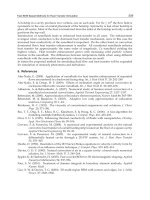
between the isotropic and anisotropic porous media. Greenkorn [29] showed experimentally
that the ratio
||
/DD
⊥
varies approximately from lower value of 3 to the higher value of 60.
He showed that this ration is a function of the flow velocity.
Experimental results by Patel and Greenkorn [29] show that the ratio
||
/DD
⊥
varies from a
lower value of about 3 to a high value of about 60. This ratio of longitudinal to transverse
dispersion coefficients is shown to be actually a function of the velocity of flow. Although

the Whitaker’s method is at variance with Greenkorn experimental results, it still do give the
correct lower limit result for a homogeneous, uniform, isotropic medium.
4. References
[1] Rudd CD, Long AC, Kendall KN, Mangin CGE. Liquid molding technologies. Woodhead
Publishing Ltd; 1997.
[2] Chan, A.W. and S T. Hwang, Modeling Nonisothermal Impregnation of Fibrous Media
with Reactive Polymer Resin, Polymer Engineering & Science, 1992. 32(5):p. 310-
318.
[3] Chiu, H T., B. Yu, S.C. Chen, et al., Heat Transfer During Flow and Resin Reaction
through Fiber Reinforcement. Chemical Engineering Science, 2000. 55(17): p. 3365-
3376.
[4] Lee, L.J., W.B. Young, and R.J. Lin, Mold Filling and Cure Modeling of RTM and Srim
Processes. Composite Structures, 1994. 27(1-2): p. 109-120.
[5] Lin, R.J., L.J. Lee, and M.J. Liou, Mold Filling and Curing Analysis Liquid Composite
Molding. Polymer Composites, 1993. 14(1): p. 71-81.
[6] Tucker, C.L. and R.B. Dessenberger, Governing Equations for Flow through Stationary
Fiber Beds, in Flow and Rheology in Polymer Composites Manufacturing, S.G.
Advani, Editor. 1994, Elsevier.
[7] Lam, Y.C., S.C. Joshi, and X.L. Liu, Numerical Simulation of the Mould-Filling Process in
Resin-Transfer Moulding. Composites Science and Technology, 2000. 60(6): p. 845-
855.
[8] Wu, C.H., H T. Chiu, L.J. Lee, et al., Simulation of Reactive Liquid Composite Molding
Using an Eulerian–Lagrangian Approach. International Polymer Processing,
1998(4): p. 398-397.
[9] Bruschke, M.V. and S.G. Advani, Numerical Approach to Model Non-Isothermal Viscous
Flow through Fibrous Media with Free Surfaces. International Journal for
Numerical Methods in Fluids, 1994. 19(7): p. 575-603.
[10] Dessenberger, R.B. and C.L. Tucker, Thermal Dispersion in Resin Transfer Molding.
Polymer Composites, 1995. 16(6): p. 495-506.
Heat Transfer - Mathematical Modelling, Numerical Methods and Information Technology

642
[11] Kang, M.K., W. Lee, II, J.Y. Yoo, et al., Simulation of Mold Filling Process During Resin
Transfer Molding. Journal of Materials Processing and Manufacturing Science,
1995. 3(3): p. 297-313.
[12] Liu, B. and S.G. Advani, Operator Splitting Scheme for 3-D Temperature Solution Based
on 2-D Flow Approximation. Computational Mechanics, 1995. 16(2): p. 74-82.
[13] Mal, O., A. Couniot, and F. Dupret, Non-Isothermal Simulation of the Resin Transfer
Moulding Process. Composites - Part A: Applied Science and Manufacturing, 1998.
29(1-2): p. 189-198.
[14] Ngo, N.D. and K.K. Tamma, Non-Isothermal '2-D Flow/3-D Thermal' Developments
Encompassing Process Modeling of Composites: Flow/Thermal/Cure
Formulations and Validations. American Society of Mechanical Engineers, Applied
Mechanics Division, AMD, 1999. 233: p. 83-102
[15] Shojaei, A., S.R. Ghaffarian, and S.M.H. Karimian, Simulation of the Three- Dimensional
Non-Isothermal Mold Filling Process in Resin Transfer Molding. Composites
Science and Technology, 2003. 63(13): p. 1931-1948.
[16] Shojaei, A., S.R. Ghaffarian, and S.M.H. Karimian, Three-Dimensional Process Cycle
Simulation of Composite Parts Manufactured by Resin Transfer Molding.
Composite Structures, 2004. 65(3-4): p. 381-390.
[17] Young, W B., Three-Dimensional Nonisothermal Mold Filling Simulations in Resin
Transfer Molding. Polymer Composites, 1994. 15(2): p. 118-127.
[18] Young, W B., Thermal Behaviors of the Resin and Mold in the Process of Resin Transfer
Molding. Journal of Reinforced Plastics and Composites, 1995. 14(4): p. 310.
[19] Pillai, K.M. and M.S. Munagavalasa, Governing Equations for Unsaturated Flow
through Woven Fiber Mats. Part 2. Non-Isothermal Reactive Flows. Composites
Part A: Applied Science and Manufacturing, 2004. 35(4): p. 403-415.
[20] Phelan, F.R., Jr. Modeling of Microscale Flow in Fibrous Porous Media. 1991. Detroit,
MI, USA: Publ by Springer-Verlag New York Inc., New York, NY, USA.
[21] Donald A. Nield and Adrinan Bejan, Convection in Porous Media, Springer, 3rd edition.

[22] Robert A. Greenkorn, Flow phenomena in porous media, Marcel Dekker, INC., New
York and Besel, 1983.
[23] Rubin, H., Heat dispersion effect on thermal convection in a porous medium layer. J.
Hydrol. 21, 1074,P: 173–184.
[24] Nikolaevskii, V.N., Convective diffusion in porous media, Journal of applied
mathematics and mechanics, 23, 6, 1492-1503, 1959.
[25] Bear, J., On the Tensor Form of Dispersion in Porous Media. Journal of Geophysical
Research, 1961. 66: p. 1185-1197.
[26] Scheidegger, A.E., General Theory of Dispersion in Porous Media. Journal of
Geophysical Research, 1961. 66(10): p. 3273-3278.
[27] Poreh, M., The Dispersivity Tensor in Isotropic and Axisymmetric Mediums. Journal of
Geophysical Research, 1965. 70: p. 3909-3913.
[28] Whitaker, S., Diffusion and Dispersion in Porous Media. AIChE Journal, 1967. 13(3): p.
420-427.
[29] Patel, R.D. and R.A. Greenkorn, On Dispersion in Laminar Flow through Porous Media.
AIChE Journal, 1970. 16(2): p. 332-334.
[30] Beavers, G.S. and Joseph D.D., Boundary condition at a naturally permeable wall, J.
Fluid Mech,. Vol. 30, pp. 197-207, 1967.
[31] Sahraoui, M. and Kaviany, M., Slip and no-slip boundary condition at interface of
porous plain media, Int. J. Heat Mass Transfer, Vol. 35, pp. 927-943, 1992.