báo cáo hóa học:" Improving energy efficiency through multimode transmission in the downlink MIMO systems" docx
Bạn đang xem bản rút gọn của tài liệu. Xem và tải ngay bản đầy đủ của tài liệu tại đây (443.47 KB, 28 trang )
This Provisional PDF corresponds to the article as it appeared upon acceptance. Fully formatted
PDF and full text (HTML) versions will be made available soon.
Improving energy efficiency through multimode transmission in the downlink
MIMO systems
EURASIP Journal on Wireless Communications and Networking 2011,
2011:200 doi:10.1186/1687-1499-2011-200
Jie Xu ()
Ling Qiu ()
Chengwen Yu ()
ISSN 1687-1499
Article type Research
Submission date 22 February 2011
Acceptance date 9 December 2011
Publication date 9 December 2011
Article URL />This peer-reviewed article was published immediately upon acceptance. It can be downloaded,
printed and distributed freely for any purposes (see copyright notice below).
For information about publishing your research in EURASIP WCN go to
/>For information about other SpringerOpen publications go to
EURASIP Journal on Wireless
Communications and
Networking
© 2011 Xu et al. ; licensee Springer.
This is an open access article distributed under the terms of the Creative Commons Attribution License ( />which permits unrestricted use, distribution, and reproduction in any medium, provided the original work is properly cited.
1
Improving energy efficiency through
multimode transmission in the downlink
MIMO systems
Jie Xu
1
, Ling Qiu
∗1
and Chengwen Yu
2
1
Personal Communication Network & Spread Spectrum Laboratory (PCN&SS), University of Science
and Technology of China (USTC), Hefei, 230027 Anhui, China
2
Wireless research, Huawei Technologies Co. Ltd., Shanghai, China
∗
Corresponding author:
Email addresses:
JX:
CY:
Abstract
Adaptively adjusting system parameters including bandwidth, transmit power and mode to maximize the “Bits
per-Joule” energy efficiency (BPJ-EE) in the downlink MIMO systems with imperfect channel state information at
the transmitter (CSIT) is considered in this article. By mode, we refer to choice of transmission schemes i.e., singular
value decomposition (SVD) or block diagonalization (BD), active transmit/receive antenna number and active user
number. We derive optimal bandwidth and transmit power for each dedicated mode at first, in which accurate capacity
estimation strategies are proposed to cope with the imperfect CSIT caused capacity prediction problem. Then, an
ergodic capacity-based mode switching strategy is proposed to further improve the BPJ-EE, which provides insights
into the preferred mode under given scenarios. Mode switching compromises different power parts, exploits the trade-
off between the multiplexing gain and the imperfect CSIT caused inter-user interference and improves the BPJ-EE
2
significantly.
Keywords: Bits per-Joule energy efficiency (BPJ-EE); downlink MIMO systems; singular value decomposition (SVD);
block diagonalization (BD); imperfect CSIT.
1. Introduction
Energy efficiency is becoming increasingly important for the future radio access networks due to the climate
change and the operator’s increasing operational cost. As base stations (BSs) take the main parts of the energy
consumption [1, 2], improving the energy efficiency of BS is significant. Additionally, multiple-input multiple-output
(MIMO) has become the key technology in the next generation broadband wireless networks such as WiMAX and
3GPP-LTE. Therefore, we will focus on the maximizing energy efficiency problem in the downlink MIMO systems
in this article.
Previous works mainly focused on maximizing energy efficiency in the single-input single-output (SISO) systems
[3–7] and point to point single user (SU) MIMO systems [8–10]. In the uplink TDMA SISO channels, the optimal
transmission rate was derived for energy saving in the non-real time sessions [3]. Miao et al. [4–6] considered
the optimal rate and resource allocation problem in OFDMA SISO channels. The basic idea of [3–6] is finding an
optimal transmission rate to compromise the power amplifier (PA) power, which is proportional to the transmit power,
and the circuit power which is independent of the transmit power. Zhang et al. [7] extended the energy efficiency
problem to a bandwidth variable system and the bandwidth–power–energy efficiency relations were investigated. As
the MIMO systems can improve the data rates compared with SISO/SIMO, the transmit power can be reduced under
the same rate. Meanwhile, MIMO systems consume higher circuit power than SISO/SIMO due to the multiplicity of
associated circuits such as mixers, synthesizers, digital-to-analog converters (DAC), filters, etc. [8] is the pioneering
work in this area that compares the energy efficiency of Alamouti MIMO systems with two antennas and SIMO
systems in the sensor networks. Kim et al. [9] presented the energy-efficient mode switching between SIMO and two
antenna MIMO systems. A more general link adaptation strategy was proposed in [10] and the system parameters
including the number of data streams, number of transmit/receive antennas, use of spatial multiplexing or space
time block coding (STBC), bandwidth, etc. were controlled to maximize the energy efficiency. However, to the
best of our knowledge, there are few works considering energy efficiency of the downlink multiuser (MU) MIMO
systems.
3
The number of transmit antennas at BS is always larger than the number of receive antennas at the mobile
station (MS) side because of the MS’s size limitation. MU-MIMO systems can provide higher data rates than SU-
MIMO by transmitting to multiple MSs simultaneously over the same spectrum. Previous studies mainly focused
on maximizing the spectral efficiency of MU-MIMO systems, some examples of which are [11–18]. Although not
capacity achieving, block diagonalization (BD) is a popular linear precoding scheme in the MU-MIMO systems
[11–14]. Performing precoding requires the channel state information at the transmitter (CSIT) and the accuracy
of CSIT impacts the performance significantly. The imperfect CSIT will cause inter-user interference and the
spectral efficiency will decrease seriously. In order to compromise the spatial multiplexing gain and the inter-user
interference, spectral efficient mode switching between SU-MIMO and MU-MIMO was presented in [15–18].
Maximizing the ”Bits per-Joule” energy efficiency (BPJ-EE) in the downlink MIMO systems with imperfect CSIT
is addressed in this article. A three part power consumption model is considered. By power conversion (PC) power,
we refer to power consumption proportional to the transmit power, which captures the effect of PA, feeder loss, and
extra loss in transmission related cooling. By static power, we refer to the power consumption which is assumed
to be constant irrespective of the transmit power, number of transmit antennas and bandwidth. By dynamic power,
we refer to the power consumption including the circuit power, signal processing power, etc., and it is assumed to
be irrespective of the transmit power but dependent on the number of transmit antennas and bandwidth. We divide
the dynamic power into three parts. The first part ”Dyn-I” is proportional to the transmit antenna number only,
which can be viewed as the circuit power. The second part ”Dyn-II” is proportional to the bandwidth only, and the
third part ”Dyn-III” is proportional to the multiplication of the bandwidth and transmit antenna number. ”Dyn-II”
and ”Dyn-III” can be viewed as the signal processing power, etc. Interestingly, there are two main trade-offs here.
For one thing, more transmit antennas would increase the spatial multiplexing and diversity gain that leads to
transmit power saving, while more transmit antennas would increase ”Dyn-I” and ”Dyn-III” leading to dynamic
power wasting. For another, multiplexing more active users with higher multiplexing gain would increase the inter-
user interference, in which the multiplexing gain makes transmit power saving, but inter-user interference induces
transmit power wasting. In order to maximize BPJ-EE, the trade-off among PC, static and dynamic power needs
to be resolved and the trade-off between the multiplexing gain and imperfect CSIT caused inter-user interference
also needs to be carefully studied. The optimal adaptation which adaptively adjusts system parameters such as
4
bandwidth, transmit power, use of singular value decomposition (SVD) or BD, number of active transmit/receive
antennas, number of active users is considered in this article to meet the challenge.
The contributions of this paper are listed as follows. By mode, we refer to the choice of transmission schemes
i.e., SVD or BD, active transmit/receive antenna number and active user number. For each dedicated mode, we
prove that the BPJ-EE is monotonically increasing as a function of bandwidth under the optimal transmit power
without maximum power constraint. Meanwhile, we derive the unique globally optimal transmit power with a
constant bandwidth. Therefore, the optimal bandwidth is chosen to use the whole available bandwidth and the
optimal transmit power can be correspondingly obtained. However, due to imperfect CSIT, it is emphasized that the
capacity prediction is a big challenge during the above derivation. To cope with this problem, a capacity estimation
mechanism is presented and accurate capacity estimation strategies are proposed.
The derivation of the optimal transmit power and bandwidth reveals the relationship between the BPJ-EE and the
mode. Applying the derived optimal transmit power and bandwidth, mode switching is addressed then to choose the
optimal mode. An ergodic capacity-based mode switching algorithm is proposed. We derive the accurate close-form
capacity approximation for each mode under imperfect CSIT at first and calculate the optimal BPJ-EE of each
mode based on the approximation. Then, the preferred mode can be decided after comparison. The proposed mode
switching scheme provides guidance on the preferred mode under given scenarios and can be applied off-line.
Simulation results show that the mode switching improves the BPJ-EE significantly and it is promising for the
energy-efficient transmission.
The rest of the article is organized as follows. Section 2 introduces the system model, power model and two
transmission schemes and then Section 3 gives the problem definition. Optimal bandwidth, transmit power derivation
for each dedicated mode and capacity estimation under imperfect CSIT are presented in Section 4. The ergodic
capacity-based mode switching is proposed in Section 5. The simulation results are shown in Section 6 and, finally,
section 7 concludes this article.
Regarding the notation, boldface letters refer to vectors (lower case) or matrices (upper case). Notation E(A)
and Tr(A) denote the expectation and trace operation of matrix A, respectively. The superscript H and T represent
the conjugate transpose and transpose operation, respectively.
5
2. Preliminaries
A. System model
The downlink MIMO systems consist of a single BS with M antennas and K users each with N antennas.
M ≥ K × N is assumed. We assume that the channel matrix from the BS to the kth user at time n is H
k
[n] ∈
C
N×M
, k = 1, . . . , K, which can be denoted as
H
k
[n] = ζ
k
ˆ
H
k
[n] = Φd
−λ
k
Ψ
ˆ
H
k
[n].
(1)
ζ
k
= Φd
−λ
k
Ψ is the large-scale fading including path loss and shadowing fading, in which d
k
, λ denote the distance
from the BS to the user k and the path loss exponent, respectively. The random variable Ψ accounts for the
shadowing process. The term Φ denotes the path loss parameter to further adapt the model, which accounts for the
BS and MS antenna heights, carrier frequency, propagation conditions and reference distance.
ˆ
H
k
[n] denotes the
small-scale fading channel. We assume that the channel experiences flat fading and
ˆ
H
k
[n] is well modeled as a
spatially white Gaussian channel, with each entry CN(0, 1).
For the kth user, the received signal can be denoted as
y
k
[n] = H
k
[n] x [n] + n
k
[n],
(2)
in which x[n] ∈ C
M×1
is the BS’s transmitted signal, n
k
[n] is the Gaussian noise vector with entries distributed
according to CN(0, N
0
W ), where N
0
is the noise power density and W is the carrier bandwidth. The design of
x[n] depends on the transmission schemes which would be introduced in Subsection 2-C.
As one objective of this article is to study the impact of imperfect CSIT, we will assume perfect channel state
information at the receive (CSIR) and imperfect CSIT here. CSIT is always got through feedback from the MSs in
the FDD systems and through uplink channel estimation based on uplink–downlink reciprocity in the TDD systems,
so the main sources of CSIT imperfection come from channel estimation error, delay and feedback error [15–17].
Only the delayed CSIT imperfection is considered in this paper, but note that the delayed CSIT model can be
simply extended to other imperfect CSIT case such as estimation error and analog feedback [15,16]. The channels
will stay constant for a symbol duration and change from symbol to symbol according to a stationary correlation
model. Assume that there is D symbols delay between the estimated channel and the downlink channel. The current
6
channel H
k
[n] = ζ
k
ˆ
H
k
[n] and its delayed version H
k
[n −D] = ζ
k
ˆ
H
k
[n −D] are jointly Gaussian with zero mean
and are related in the following manner [16].
ˆ
H
k
[n] = ρ
k
ˆ
H
k
[n − D] +
ˆ
E
k
[n],
(3)
where ρ
k
denotes the correlation coefficient of each user,
ˆ
E
k
[n] is the channel error matrix, with i.i.d. entries
CN(0,
2
e,k
) and it is uncorrelated with
ˆ
H
k
[n −D]. Meanwhile, we denote E
k
[n] = ζ
k
ˆ
E
k
[n]. The amount of delay
is τ = DT
s
, where T
s
is the symbol duration. ρ
k
= J
0
(2πf
d,k
τ) with Doppler spread f
d,k
, where J
0
(·) is the
zeroth order Bessel function of the first kind, and
2
e,k
= 1 − ρ
2
k
[16]. Therefore, both ρ
k
and
e,k
are determined
by the normalized Doppler frequency f
d,k
τ.
B. Power model
Apart from PA power and the circuit power, the signal processing, power supply and air-condition power should
also be taken into account at the BS [19]. Before introduction, assume the number of active transmit antennas is
M
a
and the total transmit power is P
t
. Motivated by the power model in [19,7,10], the three part power model is
introduced as follows. The total power consumption at BS is divided into three parts. The first part is the PC power
P
PC
=
P
t
η
,
(4)
in which η is the PC efficiency, accounting for the PA efficiency, feeder loss and extra loss in transmission related
cooling. Although the total transmit power should be varied as M
a
and W changes, we study the total transmit
power as a whole and the PC power includes all the total transmit power. The effect of M
a
and W on the transmit
power independent power is expressed by the second part: the dynamic power P
Dyn
. P
Dyn
captures the effect of
signal processing, circuit power, etc., which is dependent on M
a
and W , but independent of P
t
. P
Dyn
is separated
into three classes. The first class ”Dyn-I” P
Dyn−I
is proportional to the transmit antenna number only, which can
be viewed as the circuit power of the RF. The second part ”Dyn-II” P
Dyn−II
is proportional to the bandwidth only,
and the third part ”Dyn-III” P
Dyn−III
is proportional to the multiplication of the bandwidth and transmit antenna
number. P
Dyn−II
and P
Dyn−III
can be viewed as the signal processing related power. Thus, the dynamic power can
7
be denoted as follows.
P
Dyn
= P
Dyn−I
+ P
Dyn−II
+ P
Dyn−III
,
P
Dyn−I
= M
a
P
cir
,
P
Dyn−II
= p
ac,bw
W,
P
Dyn−III
= M
a
p
sp,bw
W,
(5)
The third part is the static power P
Sta
, which is independent of P
t
, M
a
, and W , including the power consumption
of cooling systems, power supply and so on. Combining the three parts, we have the total power consumption as
follows:
P
total
= P
PC
+ P
Dyn
+ P
Sta
.
(6)
Although the above power model is simple and abstract, it captures the effect of the key parameters such as P
t
, M
a
,s
and W and coincides with the previous literature [19, 7,10]. Measuring the accurate power model for a dedicated
BS is very important for the research of energy efficiency, and the measuring may need careful field test; however,
it is out of scope here.
Note that here we omit the power consumption at the user side, as the users’ power consumption is negligible
compared with the power consumption of BS. Although any BS power saving design should consider the impact
to the users’ power consumption, it is beyond the scope of this article.
C. Transmission schemes
Single user (SU)-MIMO with SVD and MU-MIMO with BD are considered in this article as the transmission
schemes. We will introduce them in this subsection.
1) SU-MIMO with SVD: Before discussion, we assume that M
a
transmit antennas are active in the SU-MIMO.
As more active receive antennas result in transmit power saving due to higher spatial multiplexing and diversity
gain, N antennas should be all active at the MS side.
a
The number of data streams is limited by the minimum
number of transmit and receive antennas, which is denoted as N
s
= min(M
a
, N).
In the SU-MIMO mode, SVD with equal power allocation is applied. Although SVD with waterfilling is the
capacity optimal scheme [20], considering equal power allocation here helps in the comparison between SU-MIMO
8
and MU-MIMO fairly [16]. The SVD of H[n] is denoted as
H[n] = U[n]Λ[n]V[n]
H
,
(7)
in which Λ[n] is a diagonal matrix, U[n] and V[n] are unitary. The precoding matrix is designed as V[n] at the
transmitter in the perfect CSIT scenario. However, when only the delayed CSIT is available at the BS, the precoding
matrix is based on the delayed version, which should be V[n −D]. After the MS preforms MIMO detection, the
achievable capacity can be denoted as
R
s
(M
a
, P
t
, W) = W
N
s
i=1
log
1 +
P
t
N
s
N
0
W
λ
2
i
,
(8)
where λ
i
is the ith singular value of H[n]V[n − D].
2) MU-MIMO with BD: We assume that K
a
users each with N
a,i
, i = 1, . , K
a
antennas are active at the same
time. Denote the total receive antenna number as N
a
=
K
a
i=1
N
a,i
. As linear precoding is preformed, we have that
M
a
≥ N
a
[11], and then the number of data streams is N
s
= N
a
. The BD precoding scheme with equal power
allocation is applied in the MU-MIMO mode. Assume that the precoding matrix for the kth user is T
k
[n] and the
desired data for the kth user is s
k
[n], then x[n] =
K
a
i=1
T
i
[n]s
i
[n]. The transmission model is
y
k
[n] = H
k
[n]
K
a
i=1
T
i
[n]s
i
[n] + n
k
[n].
(9)
In the perfect CSIT case, the precoding matrix is based on H
k
[n]
K
a
i=1,i=k
T
i
[n] = 0. The detail of the design can
be found in [11]. Define the effective channel as H
eff,k
[n] = H
k
[n]T
k
[n]. Then the capacity can be denoted as
R
P
b
(M
a
, K
a
, N
a,1
, . . . , N
a,K
a
, P
t
, W) =
W
K
a
k=1
log det
I +
P
t
N
s
N
0
W
H
eff,k
[n]H
H
eff,k
[n]
.
(10)
In the delayed CSIT case, the precoding matrix design is based on the delayed version, i.e., H
k
[n−D]
K
a
i=1,i=k
T
(D)
i
[n] =
0. Then define the effective channel in the delayed CSIT case as
ˆ
H
eff,k
[n] = H
k
[n]T
(D)
k
[n]. The capacity can be
denoted as [16]
R
D
b
(M
a
, K
a
, N
a,1
, . . . , N
a,K
a
, P
t
, W) =
W
K
a
k=1
log det
I +
P
t
N
s
ˆ
H
eff,k
[n]
ˆ
H
H
eff,k
[n]R
−1
k
[n]
,
(11)
in which
R
k
[n] =
P
t
Ns
E
k
[n]
i=k
T
(D)
i
[n]T
(D)H
i
[n]
E
H
k
[n] + N
0
W I (12)
is the inter-user interference plus noise part.
9
3. Problem definition
The objective of this article is to maximize the BPJ-EE in the downlink MIMO systems. The BPJ-EE is defined
as the achievable capacity divided by the total power consumption, which is also the transmitted bits per unit energy
(Bits/Joule). Denote the BPJ-EE as ξ and then the optimization problem can be denoted as
max ξ =
R
m
(M
a
,K
a
,N
a,1
, ,N
a,K
a
,P
t
,W )
P
total
s.t. P
TX
≥ 0,
0 ≤ W ≤ W
max
.
(13)
According to the above problem, bandwidth limitation is considered. In order to make the transmission most energy
efficient, we should adaptively adjust the following system parameters: transmission scheme m ∈ {s, b}, i.e., use
of SVD or BD, number of active transmit antennas M
a
, number of active users K
a
, number of receive antennas
N
a,i
, i = 1, . , K
a
, transmit power P
t
and bandwidth W .
The optimization of problem (13) is divided into two steps. At first, determine the optimal P
t
and W for each
dedicated mode. After that, apply mode switching to determine the optimal mode, i.e., optimal transmission scheme
m, optimal transmit antenna number M
a
, optimal user number K
a
and optimal receive antenna number N
a,i
,
according to the derivations of the first step. The next two sections will describe the details.
4. Maximizing energy efficiency with optimal bandwidth and transmit power
The optimal bandwidth and transmit power are derived in this section under a dedicated mode. Unless otherwise
specified, the mode, i.e., transmission scheme m, active transmit antenna number M
a
, active receive antenna number
N
a,i
, i = 1, . . . , K
a
and active user number K
a
, is constant in this section. The following lemma is introduced at
first to help in the derivation.
Lemma 1: For optimization problem
max
f(x)
ax+b
,
s.t. x ≥ 0
(14)
in which a > 0 and b > 0. f(x) ≥ 0 (x ≥ 0) and f(x) is strictly concave and monotonically increasing. There
exists a unique globally optimal x
∗
given by
x
∗
=
f(x
∗
)
f
(x
∗
)
−
b
a
,
(15)
10
where f
(x) is the first derivative of function f(x).
Proof: See Appendix A.
A. Optimal energy-efficient bandwidth
To illustrate the effect of bandwidth on the BPJ-EE, the following theorem is derived.
Theorem 1: Under constant P
t
, there exists a unique globally optimal W
∗
given by
W
∗
=
(P
PC
+ P
Sta
+ M
a
P
cir
) + (M
a
p
sp,bw
+ P
ac,bw
)R(W
∗
)
(M
a
p
sp,bw
+ P
ac,bw
)R
(W
∗
)
(16)
to maximize ξ, in which R(W ) denotes the achievable capacity with a dedicated mode. If the transmit power scales
as P
t
= p
t
W , ξ is monotonically increasing as a function of W .
Proof: See Appendix B.
This theorem provides helpful insights into the system configuration. When the transmit power of BS is fixed,
configuring the optimal bandwidth helps improve the energy efficiency. Meanwhile, if the transmit power can
increase proportionally as a function of bandwidth based on P
t
= p
t
W , transmitting over the whole available
spectrum is thus the optimal energy-efficient transmission strategy. As P
t
can be adjusted in problem (13) and no
maximum transmit power constraint is considered there, and choosing W
∗
= W
max
as the optimal bandwidth can
maximize ξ. Therefore, W
∗
= W
max
is applied in the rest of this article.
One may argue that the transmit power is limited by the BS’s maximum power in the real systems. In that case,
W and P
t
should be jointly optimized. We consider this problem in our another work [21].
B. Optimal energy-efficient transmit power
After determining the optimal bandwidth, we should derive the optimal P
∗
t
under W
∗
= W
max
. In this case, we
denote the capacity as R(P
t
) with the dedicated mode. Then the optimal transmit power is derived according to
the following theorem.
Theorem 2: There exists a unique globally optimal transmit power P
∗
t
of the BPJ-EE optimization problem given
by
P
∗
t
=
R(P
∗
t
)
R
(P
∗
t
)
− η(P
Sta
+ P
Dyn
).
(17)
Proof: See Appendix C.
11
Therefore, the optimal bandwidth and transmit power are derived based on Theorems 1 and 2. That is to say, the
optimal bandwidth is chosen as W
∗
= W
max
and the optimal transmit power is derived according to (17).
However, note that during the optimal transmit power derivation (17), the BS needs to know the achievable
capacity-based on the CSIT prior to the transmission. If perfect CSIT is available at BS, the capacity formula can
be calculated at the BS directly according to (8) for SU-MIMO with SVD and (10) for MU-MIMO with BD.
But if the CSIT is imperfect, the BS needs to predict the capacity then. In order to meet the challenge, a capacity
estimation mechanism with delayed version of CSIT is developed, which is the main concern of the next subsection.
C. Capacity estimation under imperfect CSIT
1) SU-MIMO: SU-MIMO with SVD is relatively robust to the imperfect CSIT [16], and using the delayed
version of CSIT directly is a simple and direct way. The following proposition shows the capacity estimation of
SVD mode.
Proposition 1: The capacity estimation of SU-MIMO with SVD is directly estimated by:
R
est
s
= W
N
s
i=1
log
1 +
P
t
N
s
N
0
W
˜
λ
2
i
,
(18)
where
˜
λ
i
is the singular value of H[n − D].
Proposition 1 is motivated by [16]. In Proposition 1, when the receive antenna number is equal to or larger than
the transmit antenna number, the degree of freedom can be fully utilized after the receiver’s detection, and then the
ergodic capacity of (18) would be the same as the delayed CSIT case in (8). When the receive antenna number
is smaller than the transmit antenna number, although delayed CSIT would cause degree of freedom loss and (18)
cannot express the loss, the simulation will show that Proposition 1 is accurate enough to obtain the optimal ξ in
that case.
2) MU-MIMO: Since the imperfect CSIT leads to inter-user interference in the MU-MIMO systems, simply
using the delayed CSIT cannot accurately estimate the capacity any longer. We should take the impact of inter-user
interference into account. Zhang et al. [16] first considered the performance gap between the perfect CSIT case
and the imperfect CSIT case, which is described as the following lemma.
12
Lemma 2: The rate loss of BD with the delayed CSIT is upper bounded by [16]:
R
b
= R
P
b
− R
D
b
≤ R
upp
b
=
W
K
a
k=1
N
a,k
log
2
K
a
i=1,i=k
N
a,i
P
t
ζ
k
N
0
W N
s
2
e,k
+ 1
.
(19)
As the BS can get the statistic variance of the channel error
2
e,k
due to the Doppler frequency estimation, the
BS can obtain the upper bound gap R
upp
b
through some simple calculation. According to Proposition 1, we can
use the delayed CSIT to estimate the capacity with perfect CSIT R
P
b
and we denote the estimated capacity with
perfect CSIT as
R
est,P
b
=
W
K
a
k=1
log det
I +
P
t
N
s
N
0
W
H
eff,k
[n − D]H
H
eff,k
[n − D]
,
(20)
in which H
eff,k
[n −D] = H
k
[n −D]T
k
[n −D]. Combining (20) and Lemma 2, a lower bound capacity estimation
is denoted as the perfect case capacity R
est,P
b
minus the capacity upper bound gap R
upp
b
, which can be denoted
as [18]
R
est−Zhang
b
= R
est,P
b
− R
upp
b
.
(21)
However, this lower bound is not tight enough; a novel lower bound estimation and a novel upper bound estimation
are proposed to estimate the capacity of MU-MIMO with BD.
Proposition 2: The lower bound of the capacity estimation of MU-MIMO with BD is given by (22), while the
upper bound of the capacity estimation of MU-MIMO with BD is given by (23). The lower bound in (22) is tighter
than R
est,Zhang
b
in (21).
R
est,low
b
= W
K
a
k=1
log det
I +
P
t
/N
s
N
0
W +
K
a
i=1,i=k
N
a,i
P
t
ζ
k
N
s
2
e,k
H
eff,k
[n − D]H
H
eff,k
[n − D]
(22)
R
est,upp
b
= W
K
a
k=1
log det
I +
P
t
/N
s
N
0
W +
K
a
i=1,i=k
N
a,i
P
t
ζ
k
N
s
2
e,k
H
eff,k
[n − D]H
H
eff,k
[n − D]
+ (N
a,k
/M
a
) log
2
(e)
(23)
Proposition 2 is motivated by [22]. It is illustrated as follows. Rewrite the transmission mode of user k of (9) as
y
k
[n] = H
k
[n]T
k
[n]s
k
[n] + H
k
[n]
i=k
T
i
[n]s
i
[n] + n
k
[n].
(24)
13
With delayed CSIT ,denote
B
k
[n] = H
k
[n]
i=k
T
(D)
i
[n]s
i
[n] = E
k
[n]
i=k
T
(D)
i
[n]s
i
[n],
then A
k
[n] = B
k
[n]B
H
k
[n] and the covariance matrix of the interference plus noise is then
R
k
[n] =
P
t
N
s
A
k
[n] + N
0
W I[n].
(25)
The expectation of R
k
[n] is [16]
E (R
k
[n]) =
K
a
i=1,i=k
N
a,i
P
t
ζ
k
N
s
2
e,k
I + N
0
W I
(26)
Based on Proposition 1, we use H
eff,k
[n − D] with the delayed CSIT to replace the
ˆ
H
eff,k
[n] in (11). Then the
capacity expression of each user is similar to the SU-MIMO channel with inter-stream interference. The capacity
lower bound and upper bound with a point to point MIMO channel with channel estimation errors in [22] is applied
here. Therefore, the lower bound estimation (22) and upper bound estimation (23) can be verified according to the
lower and upper bounds in [22] and (26).
We can get R
est,low
b
− R
est,Zhang
b
> 0 after some simple calculation, so R
est,low
b
is tighter than R
est,Zhang
b
.
According to Propositions 1 and 2, the capacity estimation for both SVD and BD can be performed. In order
to apply Propositions 1 and 2 to derive the optimal bandwidth and transmit power, it is necessary to prove that
the capacity estimation (18) for SU-MIMO and (22, 23) for MU-MIMO are all strictly concave and monotonically
increasing. At first, as R
est
s
in (18) is similar to R
s
(M
a
, P
t
, W) in (8), the same property of strictly concave and
monotonically increasing of (18) is fulfilled. About (22) and (23), the proof of strictly concave and monotonically
increasing is similar with the proof procedure in Theorem 2. If we denote g
k,i
> 0, i = 1, . . . , N
a,k
as the eigenvalues
of H
eff,k
[n − D]H
H
eff,k
[n − D], (22) and (23) can be rewritten as
R
est,low
b
= W
K
a
k=1
N
a,k
i=1
log
1 +
P
t
/N
s
N
0
W +
K
a
i=1,i=k
N
a,i
P
t
ζ
k
N
s
2
e,k
g
k,i
and
R
est,upp
b
= W
K
a
k=1
N
a,k
i=1
log
1 +
P
t
/N
s
N
0
W +
K
a
i=1,i=k
N
a,i
P
t
ζ
k
N
s
2
e,k
g
k,i
+ (N
a,k
/M
a
)log
2
(e)
,
respectively. Calculating the first and second derivation of the above two equations, it can be proved that (22) and
(23) are both strictly concave and monotonically increasing in P
t
and W . Therefore, based on the estimations of
Propositions 1 and 2, the optimal bandwidth and transmit power can be derived at the BS.
14
5. Energy-efficient mode switching
A. Mode switching based on instant CSIT
After getting the optimal bandwidth and transmit power for each dedicated mode, choosing the optimal mode
with optimal transmission mode m
∗
, optimal transmit antenna number M
∗
a
, optimal user number K
∗
a
each with
optimal receive antenna number N
∗
a,i
is important to improve the energy efficiency. The mode switching procedure
can be described as follows.
Energy-efficient mode switching procedure
Step 1. For each transmission mode m with dedicated active transmit antenna number M
a
, active user number
K
a
and active receive antenna number N
a,i
, calculate the optimal transmit power P
∗
t
and the corresponding BPJ-EE
according to the bandwidth W
∗
= W
max
and capacity estimation based on Propositions 1 and 2.
Step 2. Choose the optimal transmission mode m
∗
with optimal M
∗
a
, K
∗
a
and N
∗
a,i
with the maximum BPJ-EE.
The above procedure is based on the instant CSIT. As we know, there are two main schemes to choose the
optimal mode in the spectral efficient multimode transmission systems. The one is based on the instant CSIT [12–
14], while the other is based on the ergodic capacity [15–17]. The ergodic capacity-based mode switching can
be performed off-line and can provide more guidance on the preferred mode under given scenarios. If applying
the ergodic capacity of each mode in the energy-efficient mode switching, similar benefits can be exploited. The
next subsection will present the approximation of ergodic capacity and propose the ergodic capacity-based mode
switching.
B. Mode switching based on the ergodic capacity
Firstly, the ergodic capacity of each mode need to be developed. The following lemma gives the asymptotic result
of the point to point MIMO channel with full CSIT when M
a
≥ N
a
.
Lemma 3: For a point to point channel when M
a
≥ N
a
, denote β =
M
a
N
a
and γ =
P
t
ζ
k
N
0
W
[16,23]. The capacity
is approximated as
R
appro
s
≈ W C
iso
(β, βγ)
(27)
15
in which C
iso
is the asymptotic spectral efficiency of the point to point channel, and C
iso
can be denoted as
C
iso
(β,γ)
N
a
= log
2
1 + γ −F(β,
γ
β
)
+β log
2
1 +
γ
β
− F(β,
γ
β
)
− β
log
2
(e)
γ
F(β,
γ
β
)
(28)
with
F(x, y) =
1
4
1 + y(1 +
√
x)
2
−
1 + y(1 −
√
x)
2
2
.
As SVD is applied in the SU-MIMO systems, and the transmission is aligned with the maximum N
s
singular
vectors. When M
a
< N
a
, the achievable capacity approximation is modified as
R
appro
s
≈ W C
iso
(
ˆ
β,
ˆ
βγ),
(29)
where
ˆ
β =
1
β
=
N
a
M
a
.
Therefore, according to Proposition 1, the following proposition can be get directly.
Proposition 3: The ergodic capacity of SU-MIMO with SVD is estimated by:
R
Ergodic
s
= R
appro
s
.
(30)
Although Zhang et al. [16] give another accurate approximation for the MU-MIMO systems with BD, it is only
applicable in the scenario in which
K
a
i=1
N
a,i
= M
a
. We develope the ergodic capacity estimation with BD based
on Proposition 2.
As T
k
[n − D] is designed to null the inter-user interference, it is a unitary matrix independent of H
k
[n − D].
So H
k
[n − D]T
k
[n − D] is also a zero-mean complex Gaussian matrix with dimension N
a,k
× M
a,k
, where
M
a,k
= M
a
−
K
a
i=1,i=k
N
a,i
. The effective channel matrix of user k can be treated as a SU-MIMO channel with
transmit antenna number M
a,k
and receive antenna number N
a,k
. Combining Propositions 1, 2, and 3, we have the
following Proposition.
Proposition 4: The lower bound of the ergodic capacity estimation of MU-MIMO with BD is given by
R
Ergodic−low
b
≈ W
K
a
k=1
C
iso
(
ˆ
β
k
,
ˆ
β
k
ˆγ
k
),
(31)
while the upper bound of the ergodic capacity estimation of MU-MIMO with BD is given by
R
Ergodic−upp
b
≈ W
K
a
k=1
C
iso
(
ˆ
β
k
,
ˆ
β
k
ˆγ
k
) +
1
ˆ
β
k
log
2
(e)
,
(32)
16
where
ˆ
β
k
= M
a,k
/N
a,k
,
ˆγ
k
=
P
t
ζ
k
N
0
W +
K
a
i=1,i=k
N
a,i
P
t
ζ
k
N
s
2
e,k
.
For comparison, the ergodic capacity lower bound based on (21) is also considered. As shown in (19), the
expectation can be denoted as
E(R
P
b
− R
D
b
) ≤ E(R
upp
b
).
As R
upp
b
is a constant, we have E(R
upp
b
) = R
upp
b
, and then
E(R
P
b
) − E(R
D
b
) ≤ R
upp
b
.
(33)
Therefore, the lower bound estimation in (21) can also be applied to the ergodic capacity case. As the expectation
of (20) can be denoted as [16]
E(R
est,P
b
) = W
K
a
k=1
C
iso
(
ˆ
β
k
,
ˆ
β
k
γ),
(34)
the low bound ergodic capacity estimation can be denoted as
R
Ergodic−Zhang
b
≈ W
K
a
k=1
C
iso
(
ˆ
β
k
,
ˆ
β
k
γ) − R
upp
b
.
(35)
After getting the ergodic capacity of each mode, the ergodic capacity-based mode switching algorithm can be
summarized as follows.
Ergodic Capacity-Based Energy-Efficient Mode Switching
Step 1. For each transmission mode m with dedicated M
a
, K
a
and N
a,i
, calculate the optimal transmit power
P
∗
t
and the corresponding BPJ-EE according to the bandwidth W
∗
= W
max
and ergodic capacity estimation based
on Propositions 3 and 4.
Step 2. Choose the optimal m
∗
with optimal M
∗
a
, K
∗
a
and N
∗
a,i
with the maximum BPJ-EE.
According to the ergodic capacity-based mode switching scheme, the operation mode under dedicated scenarios
can be determined in advance. Saving a lookup table at the BS according to the ergodic capacity-based mode
switching, the optimal mode can be chosen simply according to the application scenarios. The performance and the
preferred mode in a given scenario will be shown in the next section.
17
6. Simulation results
This section provides the simulation results. In the simulation, M = 6, N = 2, and K = 3. All users are assumed
to be homogeneous with the same distance and moving speed. Only path loss is considered for the large-scale fading
model and the path loss model is set as 128.1+37.6 log
10
d
k
dB (d
k
in kilometers). Carrier frequency is set as 2 GHz
and D = 1 ms. Noise density is N
0
= −174 dBm/Hz. The power model is modified according to [19], which is set
as η = 0.38, P
cir
= 66.4 W, P
Sta
= 36.4 W, p
sp,bw
= 3.32 µW/Hz, and p
ac,bw
= 1.82 µW/Hz. W
max
= 5 MHz.
For simplification, “SU-MIMO (M
a
,N
a
)” denotes SU-MIMO mode with M
a
active transmit antennas and N
a
active
receive antennas, “SIMO” denotes SU-MIMO mode with one active transmit antennas and N active receive antennas
and “MU-MIMO (M
a
,N
a
,K
a
)” denotes MU-MIMO mode with M
a
active transmit antennas and K
a
users each N
a
active receive antennas. Seven transmission modes are considered in the simulation, i.e., SIMO, SU-MIMO (2,2),
SU-MIMO (4,2), SU-MIMO (6,2), MU-MIMO (4,2,2), MU-MIMO (6,2,2), MU-MIMO (6,2,3). In the simulation,
the solution of (15)–(17) is derived by the Newton’s method, as the close-form solution is difficult to obtain.
Figure 1 depicts the effect of capacity estimation on the optimal BPJ-EE under different moving speed. The
optimal estimation means that the BS knows the channel error during calculating P
∗
t
and the precoding is still
based on the delayed CSIT. In the left figure, SU-MIMO is plotted. The performance of capacity estimation and
the optimal estimation are almost the same, which indicates that the capacity estimation of the SU-MIMO systems
is robust to the delayed CSIT. Another observation is that the BPJ-EE is nearly constant as the moving speed is
increasing for SIMO and SU-MIMO (2,2), while it is decreasing for SU-MIMO (4,2) and SU-MIMO (6,2). The
reason can be illustrated as follows. The precoding at the BS cannot completely align with the singular vectors of
the channel matrix under the imperfect CSIT. But when the transmit antenna number is equal to or greater than the
receive antenna number, the receiver can perform detection to get the whole channel matrix’s degree of freedom.
However, when the transmit antennas are less than the receive antenna, the receiver cannot get the whole degree of
freedom only through detection, so the degree of freedom loss occurs. The center and right figures show us the effect
of capacity estimation with MU-MIMO modes. The three estimation schemes all track the effect of imperfect CSIT.
From the amplified sub-figures, the upper bound capacity estimation is the closest one to the optimal estimation.
It indicates that the upper bound capacity estimation is the best one in the BD scheme. Moreover, we can see that
BPJ-EE of the BD scheme decreases seriously due to the imperfect CSIT caused inter-user interference.
Figure 4 demonstrates the preferred transmission mode under the given scenarios. The optimal mode under
According to Figures 1 and 2, the upper bound estimation is the best estimation scheme for the MU-MIMO mode.
18
Figure 2 compares the BPJ-EE derived by ergodic capacity estimation schemes and the one by simulations. The
left figure demonstrates the SU-MIMO modes. The estimation of SIMO, SU-MIMO (4,2) and SU-MIMO (6,2)
is accurate when the moving speed is low. But when the speed is increasing, the ergodic capacity estimation of
SU-MIMO (4,2) and SU-MIMO (6,2) cannot track the decrease of BPJ-EE. There also exists a gap between the
ergodic capacity estimation and the simulation in the SIMO mode. Although the mismatching exists, the ergodic
capacity-based mode switching can always match the optimal mode, which will be shown in the next figure. For the
MU-MIMO modes, the two lower bound ergodic capacity estimation schemes mismatch the simulation more than
the upper bound estimation scheme. That is because the lower bound estimations cause BPJ-EE decreasing twice.
Firstly, the derived transmit power would mismatch with the exactly accurate transmit power because the derivation
is based on a bound and this transmit power mismatch will make the BPJ-EE decrease compared with the simulation.
Secondly, the lower bound estimation uses a lower bound formula to calculate the estimated BPJ-EE under the
derived transmit power, which will make the BPJ-EE decrease again. Nevertheless, the upper bound estimation has
the opposite impact on the BPJ-EE estimation during the above two steps, so it matches the simulation much better.
Therefore, during the ergodic capacity-based mode switching, the upper bound estimation is applied.
Figure 3 depicts the BPJ-EE performance of mode switching. For comparison, the optimal mode with instant
CSIT (‘Optimal’) is also plotted. The mode switching can improve the energy efficiency significantly and the
ergodic capacity-based mode switching can always track the optimal mode. The performance of ergodic capacity-
based switching is nearly the same as the optimal one. Through the simulation, the ergodic capacity-based mode
switching is a promising way to choose the most energy-efficient transmission mode.
different moving speed and distance is depicted. This figure provides insights into the PC power/dynamic power/static
power trade-off and the multiplexing gain/inter-user interference compromise. When the moving speed is low, MU-
MIMO modes are preferred and vice versa. This result is similar to the spectral efficient mode switching in [15–18].
Inter-user interference is small when the moving speed is low, so there is higher multiplexing gain of MU-MIMO
benefits. When the moving speed is high, the inter-user interference with MU-MIMO becomes significant, so SU-
MIMO which can totally avoid the interference is preferred. Let us focus on the effect of distance on the mode
trade-off between the two parts should be met. Above all, the above mode switching trends of Figure 4 externalize
19
under high moving speed case then. When distance is less than 1.7 km, SU-MIMO (2,2) is the optimal one, while
the distance is equal to 2.1 and 2.5 km, the SIMO mode is suggested. When the distance is larger than 2.5 km, the
active transmit antenna number increases as the distance increases. The reason of the preferred mode variation can
be explained as follows. The total power can be divided into PC power, transmit antenna number related power
”Dyn-I” and ”Dyn-III” and transmit antenna number independent power ”Dyn-II” and static power. The first and
third part divided by capacity would increase as the active number increases, while the second part is opposite. In
the long distance scenario, the first part will dominate the total power and then a more active antenna number is
preferred. In the short and medium distance scenario, the second and third part dominate the total power and the
the two trade-offs.
7. Conclusion
This article discusses the energy efficiency maximizing problem in the downlink MIMO systems. The optimal
bandwidth and transmit power are derived for each dedicated mode with constant system parameters, i.e., fixed trans-
mission scheme, fixed active transmit/receive antenna number and fixed active user number. During the derivation,
the capacity estimation mechanism is presented and several accurate capacity estimation strategies are proposed to
predict the capacity with imperfect CSIT. Based on the optimal derivation, ergodic capacity-based mode switching
is proposed to choose the most energy-efficient system parameters. This method is promising according to the
simulation results and provides guidance on the preferred mode over given scenarios.
Appendix A
Proof of Lemma 1
Proof: The proof of the above lemma is motivated by [4]. Denote the inverse function of y = f(x) as x = g(y),
then x
∗
= arg max
x
f(x)
ax + b
= arg max
g (y)
y
ag(y) + b
. Denote y
∗
= f (x
∗
). Since f(x) is monotonically increasing,
y
∗
= arg max
y
y
ag( y) + b
. According to [4], there exists a unique globally optimal y
∗
given by
y
∗
=
b + ag(y
∗
)
ag
(y
∗
)
(36)
if g(y) is strictly convex and monotonically increasing. (36) is fulfilled since the inverse function of g(y), i.e., f (x)
is strictly concave and monotonically increasing. Taking g
(y) =
1
f
(x)
and f(x) = y into (36), we can get (15).
20
Appendix B
Proof of Theorem 1
Proof: The first part can be proved according to Lemma 1. Calculating the first and second derivation of R(W )
based on (8), (10) and (11), we can see that R(W) of both SVD and BD mode is strictly concave and monotonically
increasing as a function of W . The optimal W
∗
can be got through (15), which is given by (16).
Look at the second part. Taking P
t
= p
t
W into (8), (10) and (11), the capacity is R(P
t
, W) = W
ˆ
R
m
(p
t
), where
ˆ
R(p
t
) is independent of W. We have that
ξ =
W
ˆ
R(p
t
)
(M
a
p
sp,bw
+ p
ac,bw
)W + M
a
P
cir
+ P
PC
+ P
Sta
.
(37)
The second part is verified.
Appendix C
Proof of Theorem 2
Proof: According to Lemma 1, the above theorem can be verified if we prove that R
m
(P
t
) is strictly concave
and monotonically increasing for both SVD and BD. It is obvious that the capacity of SVD and BD with perfect
CSIT is strictly concave and monotonically increasing based on (8) and (10). If the capacity of BD with imperfect
CSIT can also be proved to be strictly concave and monotonically increasing, Theorem 2 can be proved.
Denoting A
k
= E
k
[n]
i=k
T
(D)
i
[n]T
(D)H
i
[n]
E
H
k
[n], then rewrite (11) as follows:
R
D
b
(P
t
) = W
K
a
k=1
log det
R
k
[n] +
P
t
N
s
ˆ
H
eff,k
[n]
ˆ
H
H
eff,k
[n]
− log det R
k
[n]
= W
K
a
k=1
log det
I +
P
t
N
0
W Ns
A
k
+
ˆ
H
eff,k
[n]
ˆ
H
H
eff,k
[n]
− log det
I +
P
t
N
0
W Ns
A
k
= W
K
a
k=1
N
a,k
i=1
log
1 +
P
t
N
0
W Ns
c
k,i
− log
1 +
P
t
N
0
W Ns
g
k,i
.
(38)
c
k,i
and g
k,i
are the eigenvalue of A
k
+
ˆ
H
eff,k
[n]
ˆ
H
H
eff,k
[n] and A
k
, respectively. Sorting c
k,i
and g
k,i
as c
k,1
≥
. . . ≥ c
k,N
a,k
and g
k,1
≥ . . . ≥ g
k,N
a,k
. Since A
k
and
ˆ
H
eff,k
[n]
ˆ
H
H
eff,k
[n] are both positive definite, c
k,i
> g
k,i
, i =
1, . . . , N
a,k
. Calculating the first and second derivation of (38), (11) is strictly concave and monotonically increasing.
Then Theorem 2 is verified.
Competing interests
The authors declare that they have no competing interests.
Acknowledgments
on Communications, Control and Signal Processing, ISCCSP 2010, Limassol, Cyprus, 3–5 March 2010
Vehicular Technology Conference Fall
21
This work is supported in part by Huawei Technologies Co. Ltd., Shanghai, China, Chinese Important National
Science and Technology Specific Project (2010ZX03002-003) and National Basic Research Program of China (973
Program) 2007CB310602. The authors would like to thank the anonymous reviewers for their insightful comments
and suggestions.
Endnotes
a
Here, more receive antenna at MS will cause higher MS power consumption. However, note that the power
consumption of MS is omitted.
References
[1] G Fettweis, Ernesto Zimmermann, ICT Energy Consumption - Trends And Challenges, in proc. of WPMC, 2008
[2] O Blume, D Zeller, U Barth, Approaches to Energy Efficient Wireless Access Networks, in Proceedings of the 4th International Symposium
[3] H Kim, G de Veciana, Leveraging Dynamic Spare Capacity in Wireless System to Conserve Mobile Terminals’ Energy. IEEE/ACM Trans.
Netw. 18(3), 802–815 (2010)
[4] GW Miao, N Himayat, GY Li, D Bormann, Energy-efficient design in wireless OFDMA. Proc. IEEE 2008 International Conference on
Communications, Beijing , China , May 2008, pp. 3307–3312
[5] GW Miao, N Himayat, GY Li, A Swami, Cross-layer optimization for energy-efficient wireless communications: a survey, (invited). Wiley
J Wirel Commun. Mobile Comput 9(4), 529–542 (2009)
[6] GW Miao, N Himayat, GY Li, Energy-efficient link adaptation in frequency-selective channels. IEEE Trans. Commun. 58(2), 545–554
(2010)
[7] S Zhang, Y Chen, S Xu, Improving Energy Efficiency through Bandwidth, Power, and Adaptive Modulation. IEEE Proceeding of 2010
[8] S Cui, AJ Goldsmith, A Bahai, Energy-efficiency of MIMO and cooperative MIMO techniques in sensor networks. IEEE J. Sel. Areas
Commun. 22(6), 1089–1098 (2004)
[9] H Kim, C-B Chae, G Veciana, RW Heath, A cross-layer approach to energy efficiency for adaptive MIMO systems exploiting spare
capacity. IEEE Trans. Wirel. Commun. 8(8) (2009)
[10] HS Kim, B Daneshrad, Energy-constrained link adaptation for MIMO OFDM wireless communication systems. IEEE Trans. Wirel.
Commun. 9(9), 2820–2832 (2010)
[11] QH Spencer, AL Swindlehurst, M Haardt, Zero-forcing methods for downlink spatial multiplexing in multi-user MIMO channels. IEEE
Trans. Signal Process 52(2), 461–471 (2004)
22
[12] Z Shen, R Chen, JG Andrews, RW Heath Jr., BL Evans, Low complexity user selection algorithms for multiuser MIMO systems with
block diagonalization. IEEE Trans. Signal Process. 54(9), 3658–3663 (2006)
[13] Z Shen, R Chen, JG Andrews, RW Heath Jr., BL Evans, Sum capacity of multiuser MIMO broadcast channels with block diagonalization.
IEEE Trans. Wirel. Commun. 6(6), 2040–2045 (2007)
[14] R Chen, Z Shen, JG Andrews, RW Heath Jr., Multimode transmission for multiuser MIMO systems with block diagonalization. IEEE
Trans. Signal Process. 56(7), 3294–3302 (2008)
[15] J Zhang, RW Heath Jr., M Kountouris, JG Andrews, Mode switching for the multi-antenna broadcast channel based on delay and channel
quantization. EURASIP J Adv Signal Process. 2009 15, Article ID 802548 (2009)
[16] J Zhang, JG Andrews, RW Heath Jr., Block Diagonalization in the MIMO Broadcast Channel with Delayed CSIT, in IEEE proc. of
Globecom 2009, Nov 2009, pp. 1–6
[17] J Zhang, M Kountouris, JG Andrews, RW Heath Jr., Multi-mode transmission for the MIMO broadcast channel with imperfect channel
state information. IEEE Trans. Commun. 59(3), 803–814 (2011)
[18] J Xu, L Qiu, Robust Multimode Selection in the Downlink Multiuser MIMO Channels with Delayed CSIT, in IEEE proc. of ICC 2011,
June 2011,pp. 1–5
[19] O Arnold, F Richter, G Fettweis, O Blume, Power Consumption Modeling of Different Base Station Types in Heterogeneous Cellular
Networks, in Proceedings of the ICT MobileSummit (ICT Summit’10), Florence, Italy, 16. - 18. June 2010
[20] IE Telatar, Capacity of multi-antenna Gaussian channels. Europ. Trans. Telecommun. 10, 585–595 (1999)
[21] J Xu, L Qiu, C Yu, Link Adaptation and Mode Switching for the Energy Efficient Multiuser MIMO Systems, submitted to IEICE Trans.
Commun. Available online at />∼
suming/
[22] T Yoo, AJ Goldsmith, Capacity and power allocation for fading MIMO channels with channel estimation error. IEEE Trans. Inf. Theory
52(5), 2203–2214 (2006)
[23] P Rapajic, D Popescu, Information capacity of a random signature multiple-input multiple-output channel. IEEE Trans. Commun. 48,
1245–1248 (2000)
23
Fig. 1. The effect of capacity estimation on the energy efficiency of SU-MIMO and MU-MIMO under different speed.
Fig. 2. Comparison of energy efficiency based on ergodic capacity and instant capacity with SU-MIMO and MU-MIMO.
Fig. 3. Performance of mode switching.
Fig. 4. Optimal mode under different scenario. ◦: SIMO, ×: SU-MIMO (2,2), +: SU-MIMO (4,2),: SU-MIMO (6,2),♦: MU-MIMO
(4,2,2),∇: MU-MIMO (6,2,2),: MU-MIMO (6,2,3).
Energy Efficiency(distance:1km,BW:5MHz)
Energy Efficiency(Bits/Joule)
speed(km/h)
speed(km/h)
speed(km/h)
Energy Efficiency(Bits/Joule)
Per−Joule Bits(Mbps/Joule)
Energy Efficiency(distance:1km,BW:5MHz,(6,2,3))
Energy Efficiency(distance:1km,BW:5MHz,(6,2,2))
0 10 20 30 40 50 60 70 80 90 100
1.2
1.4
1.6
1.8
2
2.2
2.4
x 10
5
Est
Opt
SIMO
SU−MIMO(2,2)
SU−MIMO(4,2)
SU−MIMO(6,2)
0 10 20 30 40 50 60 70 80 90 100
0.6
0.8
1
1.2
1.4
1.6
1.8
2
2.2
2.4
2.6
x 10
5
30 32
1.6
1.62
1.64
1.66
x 10
5
Opt
Est−Zhang
Est−Low
Est−Upp
0 10 20 30 40 50 60 70 80 90 100
0.5
1
1.5
2
2.5
3
x 10
5
19 20 21 22
1.68
1.7
1.72
1.74
x 10
5
Opt
Est−Zhang
Est−Low
Est−Upp
Figure 1