New Tribological Ways Part 8 doc
Bạn đang xem bản rút gọn của tài liệu. Xem và tải ngay bản đầy đủ của tài liệu tại đây (2.39 MB, 35 trang )
A Comparison of the Direct Compression Characteristics of Andrographis paniculata,
Eurycoma longifolia Jack, and Orthosiphon stamineus Extracts for Tablet Development
229
Fig. 5. (b) Walker plots of tablets prepared from
Eurycoma longifolia Jack, Andrographis
paniculata
and Orthosiphon stamineus for 1.0 g of feed powders.
lastly the
Andrographis paniculata extract powder. The high density gave the high value of
the tensile strength, which was related to the reduction in the void space between particles
in the powders during tablet formation with respect to the values of the slopes, which
decreased as the tensile strength increased.
Constants
Material
Feed powder (g)
W B
R
2
value
Andrographis paniculata
-0.16±0.001 2.00±0.006 0.971
Eurycoma longifolia Jack -0.24±0.001 2.33±0.056 0.984
Orthosiphon stamineus
0.5
-0.14±0.056 2.24±0.243 0.957
Andrographis paniculata
-0.14±0.002 1.99±0.000 0.948
Eurycoma longifolia Jack -0.31±0.001 2.66±0.053 0.992
Orthosiphon stamineus
1.0
-0.27±0.105 2.67±0.421 0.928
Table 4. The Walker model
4. Conclusion
This study on direct compression characteristics of selected Malaysian herb extract powders
helped to deduce and understand some of the important principles of tablet development.
The
Eurycoma longifolia Jack extract powder was the easiest of the three herb powders to
compress, and it underwent significant particle rearrangement at low compression
pressures, resulting in low values of yield pressure. The compression characteristics of the
Eurycoma longifolia
Jack powder were consistent when validated with all of the models used.
Another significant finding showed that the characteristics of 0.5 g of feed powder are better
than for 1.0 g of feed powder, as proven from the tensile strength test; hence a more
coherent tablet can be obtained. Thus, herbal parameters are superior when screening
extract powders with the desired properties, such as plastic deformation. This study also
validated the use of Heckel, Kawakita and Lüdde, and Walker model parameters as
acceptable predictors for evaluating extract powder compression characteristics.
New Tribological Ways
230
5. Acknowledgements
This work was supported by a research grant from the Ministry of Higher Education
Malaysia, Fundamental Research Grant Scheme with project number: 5523035 and
Universiti Putra Malaysia (UPM) Research University Grant Scheme with project number:
91838. Some of the authors were sponsored by a Graduate Research Fellowship from the
UPM.
6. References
Abdul Aziz, R., Kumaresan, S., Mat Taher, Z. & Chwan Yee, F.D. (2004). Phytochemical
Processing: The Next Emerging Field In Chemical Engineering: Aspects and
Opportunities (available from
http%3a//kolmetz.com/pdf/Foo/IJKM_Phytochemical.pdf
- Accessed 20/10/2008).
Adapa, P.K., Tabil, L.G., Schoenau, G.J., Crerar, B., Sokhansanj, S. & Canada (2005).
Compression characteristics of fractionated alfafa grinds.
International Journal of
Powder Handling and Processing
14(4), 252-259, ISSN: 09347348.
Ahmad, S. (2007). Mechanical Granulation by tabletting of Eurycoma longifolia jack, B. Eng.
Hons. (Process and Food) Thesis, Universiti Putra Malaysia.
Ahmad, M., and Asmawi, M.Z. (1993). Int. Conf. on the use of Traditional Med. & Other
Natural Products in Health Care, USM. (available from
- Accessed 11/11/2008).
Carr, R.L. (1965).Evaluating flow properties of powders,
Chemical Engineering. 72, 163-167
ISSN 1385-8947.
Eggelkraut-Gottanka, A.G., Abu Abed, S., Müller, W. & Schmidt, P.C. (2002). Roller
compaction and tabletting of St. John’s Wort plant dry extract using a gap width
and force controlled roller compactor I. Study of roller compaction variables on
granule and tablet properties by a 33 factorial design.
Pharmaceutical Development
Technology,
7, 447-45, ISSN: 1083-7450.
Fell, J.T. & Newton J.M. (1970). Determination of Tablet Strength by Diametrical-
Compression Test
. International Journal of Pharmaceutics, 59, 688-691, ISSN: 0378-
5173.
Fichtnera, F., Rasmuson, A. & Alderborn. G. (2005). Particle size distribution and evolution
in tablet structure during and after compaction.
International Journal of Pharmaceutics
292, 211–225, ISSN: 0378-5173.
Hausner H.H. (1967). Friction conditions in a mass of metal powder,
International Journal of
Powder Metallurgy,
3 (4), 7-13, ISSN: 0888-7462.
Heckel, R.W. (1961). An analysis of powder compaction phenomena
. Transaction of
Metallurgy Society, AIME
, 221, 671-675, ISSN 0543-5722. 221.
Jaganath, I.B. & Ng, L.T. (2000). Herbs. In The green pharmacy of Malaysia, Jaganath, I.B.,
Vinpress Sdn. Bhd and Malaysian Agricultural Research and Development Institute, ISBN
No.967-81-0281-1, Kuala Lumpur, Malaysia.
Kawakita, K. & Lüdde, K.H. (1970/71). Some considerations on powder compression
Equations.
Powder Technology, 4, 61-68, ISSN 0032-5910.
Korhonen, O., Pohja, S., Peltonen, S., Suihko, E., Vidgren, M., Paronen, P. & Ketolainen, J.
(2002). Effects of Physical Properties for Starch Acetate Powders on Tableting.
A Comparison of the Direct Compression Characteristics of Andrographis paniculata,
Eurycoma longifolia Jack, and Orthosiphon stamineus Extracts for Tablet Development
231
Pharmaceutics Science Technology AAPS., 34, ISSN 1530-9932. (available from
http://www .apppspharmscitech. org - Accessed 21/6/2008).
Mohammed, H., Briscoe, B.J. & Pitt, K.G. (2006). The intrinsic nature and coherence of
compacted pure pharmaceutical tablets.
Powder Technology, 165, 11-21, ISSN 0032-
5910.
Nokhodchi, A. (2000). An overview of the effect of moisture on compaction and
compression.
Pharmaceutical Technology. (available www.pharmtech.com - Accessed
3/7/2007).
Nokhodchi A. (2005). An Overview of The Effect of Moisture on Compaction and
Compression.
Pharmaceutical Technology (available from www.pharmatech.com -
Accessed 20/6/2009).
Nordström, J., Welch, K., Frenning, G. & Alderborn, G. (2008). On the physical
interpretation of the Kawakita and Adams parameters derived from confined
compression of granular solids.
Powder Technology 182, 424–435 , ISSN 0032-5910.
Odeku, O. A., Awe, O.O., Popoola, B., Odeniyi, M. A. & Itiola, O. A. (2005). Compression
and Mechanical Properties of Tablet Formulations Containing Corn, Sweet Potato,
and Cocoyam Starches as Binders.
Pharmaceutical Technology, 29 (4): 82-90, ISSN:
1543-2521.
Ramakrishnan, K.N., Nagarajan, R., RamaRao, G.V. & Venkadesan, S., 1997. A
Compaction Study on Ceramic Powders
. Elsevier Material Letters, 33, 191-194,
ISSN 0167-577X.
Sambandan, T., G., Rha, C. K., Abdul Kadir, A., Aminudin, N & Mohammed Saad,
J. (2006). Bioactive Fraction of
Eurycoma Longifolia. United States Patent 0087493
A1.
Schiller, M., von der Heydt, H., März, F. & Schmidt, P.C. (2003). Enhanced processing
properties and stability of film-coated tablets prepared from roller –compacted and
ion-exchanged Eschscholtzia Californica Cham. Dry Extract,
STP Pharmaceutical
Science
, 13, 111-117, ISSN 1157-1489.
Sebhatu, T., Ahlneck, C. & Alderborn, G. (1997). The effect of moisture content on the
compression and bond-formation properties of amorphous lactose particles.
International Journal of Pharmaceutics 146, 101-114, ISSN: 0378-5173.
Shivanand, P. & Sprockel, O.L. (1992). Compaction behavior of cellulose polymers. Powder
Technology,
69, 177-184, ISSN 0032-5910.
Takeuchi, H., Nagira, S., Hiromitsu Y. & Kawashima, Y. (2004). Die wall pressure
measurement for evaluation of compaction property of pharmaceutical materials,
International Journal of Pharmaceutics, 274, 131–138, ISSN: 0378-5173.
Varthalis, S. & Pilpel, N. (1976). Anomalies in some properties of powder mixtures. Journal of
Pharmacy and Pharmacology
, 28, 415-419, ISSN: 0022-3573.
Walker, E.E. (1923). The Properties of powders- Part VI: The compressibility of powders;
Transactions of the Faraday Society, 19, 73-82, ISSN: 0014-7672.
Yamamoto, Y., Fujii, M., Watanabe, K., Tsukamoto, M., Shibata, Y., Kondoh, M. &
Watanabe, Y. (2009). Effect of powder characteristics on oral tablet disintegration.
International Journal of Pharmaceutics 365, 116–120, ISSN: 0378-5173.
Yusof, Y. A., Smith, A. C., & Briscoe, B. J. (2005). Roll compaction of maize powder. Chemical
Engineering Science
, 60 (14), 3919-3931, ISSN 0009-2509.
New Tribological Ways
232
Zhang Y., Law Y. & Chakrabarti, S. (2003). Physical Properties and Compact Analysis of
commonly Used Direct Compression.
Pharmaceutical Science Technology, 4(4), 62,
ISSN 1530-9932. (available from http://www .apppspharmscitech. org - Accessed
21/6/2008).
Part 3
Tribology and Low Friction
12
Frictional Property of Flexible Element
Keiji Imado
Oita University
Japan
1. Introduction
In the calculation of frictional force of a flexible element such as a belt, rope or cable
wrapped around the cylinder, the famous Euler's belt formula (Hashimoto, 2006) or simply
known as the belt friction equation (Joseph F. Shelley, 1990) is used. The formula is useful
for designing a belt drive or band brake (J. A. Williams, 1994). On the other hand, a belt or
rope is conveniently used to tighten a luggage to a carrier or lift up the luggage from the
carrier. In that case, for the sake of adjusting the belt length and keeping an appropriate
tension during transportation, various kinds of belt buckles are used. These belt buckles
have been devised empirically and there was no theory about why it can fix the belt. The
first purpose of this chapter is to present the theory of belt buckle clearly by considering the
self-locking mechanism generated by wrapping the belt on the belt. Making use of the belt
tension for a locking mechanism, a belt buckle with no locking mechanism can be made. The
principle and some basic property of this new belt buckle are also shown.
The self-locking of belt may occur even in the case where a belt is wrapped on an axis two or
more times. The second purpose of this chapter is to present the frictional property of belt
wrapped on an axis two and three times through deriving the formulas corresponding to an
each condition. Making use of this self-locking property of belt, a belt-type one-way clutch
can be made (Imado, 2010). The principle and fundamental property of this new clutch are
described.
As the last part of this chapter, the frictional property of flexible element wrapped on a hard
body with any contour is discussed. The frictional force can be calculated by the curvilinear
integral of the curvature with respect to line element along the contact curve.
2. Theory of belt buckle
Notation
C Magnification factor of belt tension
F Frictional force, N
F
ij
= F
ji
Frictional force between point P
i
and P
j
, N
L Distance between two cylinder centers, m
N Normal force of belt to surface, N
N
ij
= N
ji
Normal force of belt between point P
i
and P
j
, N
P
i
Boundary of contact angle
R Radius of main cylinder, m
New Tribological Ways
236
T
i
Tension of belt in i’th interval, N
r Radius of accompanied cylinder, m
μ Coefficient of friction for belt-cylinder contact
μ
b
Coefficient of friction for belt-belt contact
θ Angle
θ
i
Angle of point P
i
θ
ij
=θ
ji
Contact angle between P
i
and P
j
2.1 Friction of belt in belt buckle
Figure 1 (a) shows a cross sectional view of a belt buckle and a belt wrapped around the two
cylindrical surfaces. T
1
and T
4
(T
1
>T
4
) are tensions of the belt at both ends. There is a
double-layered part where the belt is wrapped over the belt. Figure 1 (b) shows the enlarged
view around the main axis. For simplicity, the thickness of the belt was neglected.
According to the theory of belt friction, following equations are known for belt tensions of
T
1
, T
2
and T
3
(Joseph F. Shelley, 1990).
12 34
1223
,
b
Te T TeT
μθ μθ
== (1)
T
4
’ and T
4
” are of inner belt tension at P
1
and P
2
respectively. The normal force to a small
element of the inner belt at angle θ is denoted as dN
b
, which can be written as
2
()
2
b
b
dN e T d
μθθ
θ
−
= (2)
Making use of
T
4
’ and T
4
”, the normal forces of inner belt for an each section are expressed as
(a) Belt buckle (b) Enlarged view
Fig. 1. Mechanical model of belt buckle and enlarged veiw around main axis
Frictional Property of Flexible Element
237
2
1
6
()
25 4
()
12 4
()
16 4
"
'
dN e T d
dN e T d
dN e T d
μθ θ
μθ θ
μθ θ
θ
θ
θ
−
−
−
⎫
=
⎪
⎪
=
⎬
⎪
=
⎪
⎭
(3)
The frictional force between
P
1
and P
6
is
6
16
1
16 16 4
(1)FdNeT
θ
μθ
θ
μ
==−
∫
(4)
The inner belt tension
T
4
’ is the sum of the frictional force F
16
and the belt tension T
4
.
16
4416 4
'TTFeT
μθ
=+ = (5)
The frictional force F
12
acting on the inner belt is composed of two forces denoted as F
12in
and F
12out
. The frictional force F
12in
is acting on the cylindrical surface, which is generated by
the normal forces dN
b
and
dN
12
. The normal force dN
b
is exerted from the outer belt. The
other normal force dN
12
is generated by the inner belt tension. So, F
12in
is given by
11
12 12
22
2
12 12 4
(1)(1)'
b
in b
b
T
FdNdNe eT
θθ
μθ μθ
θθ
μ
μμ
μ
=+ =−+−
∫∫
(6)
Making use of Eq. (2), the frictional force F
12out
acting on the belt-belt boundary can be
written as
1
12
2
12 2
(1)
b
out b b
FdNeT
θ
μθ
θ
μ
==−
∫
(7)
The frictional force F
12
is the sum of Eqs. (6) and (7).
12 12
12 2 4
(1)1 (1)'
b
b
Fe Te T
μθ μθ
μ
μ
⎛⎞
=−++−
⎜⎟
⎝⎠
(8)
As the belt tension T
4
” is the sum of F
12
and T
4
’ , making use of Eq. (5) and (8), T
4
” can be
written as
26 12
4124 4 2
"' (1)1
b
b
TFTeTe T
μθ μ θ
μ
μ
⎛⎞
=+= + − +
⎜⎟
⎝⎠
(9)
Making use of Eq. (3), the frictional force F
25
can be written as
2
25
5
25 25 4
(1)"FdNeT
θ
μθ
θ
μ
==−
∫
(10)
As the belt tension T
3
is the sum of F
25
and T
4
”, making use of Eqs. (9) and (10), T
3
can be
expressed as
25 26 12
3254 4 2
"(1)1
b
b
TF T e eT e T
μθ μθ μ θ
μ
μ
⎧
⎫
⎛⎞
⎪
⎪
=+= + − +
⎜⎟
⎨
⎬
⎪
⎪
⎝⎠
⎩⎭
(11)
New Tribological Ways
238
Substituting Eq. (1) into Eq. (11) to eliminate T
2
gives
()
56
12
34 25
34
()
1(1)1/
b
b
e
TT
ee
μ
θ
μθ
μθ θ
μμ
+
=
−−+
(12)
Substituting Eq. (1) into Eq. (12) to get the relation between T
1
and T
4
gives
()
12 34 56
12
34 25
()
14
()
1(1)1/
b
b
b
ee
TT
ee
μ
θμθθ
μθ
μθ θ
μμ
+
+
=
−−+
(13)
In the same manner from Eq. (1) to Eq. (13), in the case of T
1
<T
4
, corresponding relation of
Eq. (13) yields as
34 56 12 16 12
()
41
(1)1
bb
b
Te e ee T
μθ θ μθ μθ μθ
μ
μ
+
⎧
⎫
⎛⎞
⎪
⎪
=+−+
⎜⎟
⎨
⎬
⎪
⎪
⎝⎠
⎩⎭
(14)
2.2 Property of formulas of belt buckle
The validity of Eqs. (13) and (14) might be checked by supposing an extreme case of either
μ=0 or μ
b
=0. Substituting μ=0 into Eq. (13) gives
12
12
14
2
b
b
e
TT
e
μ
θ
μθ
=
−
(15)
Next, substituting μ
b
=0 into Eq. (13) gives
34 56
34 56
34 25
()
()
144
()
12
1
e
TTCeT
e
μθ θ
μθ θ
μθ θ
θμ
+
+
+
==
−
(16)
Substituting μ
b
=0 into Eq. (15) or substituting μ=0 into Eq. (16) gives T
1
=T
4
. Substituting
12
0
θ
=
into Eq. (13) to remove the double-layered segment on the ratio of belt tension yields
the conventional equation of belt friction.
34 56
()
14
Te T
μθ θ
+
= (17)
Equation (17) is also obtained by substituting
12
0
θ
=
into Eq. (16). This means that the ratio
of belt tension is magnified by the factor C
34 25
()
12
1
1
C
e
μθ θ
θμ
+
=
−
(18)
due to the double-layered segment even in the case of μ
b
=0. As far as these inspections are
concerned, there is no contradiction in Eq. (13). As Eqs. (13), (15) and (16) are of fractions,
the factor of T
4
might become infinity meaning T
4
/T
1
=0. This fact virtually implies the
occurrence of self-locking. Figure 2 shows the relation of μ
b
and θ
12
satisfying
b12
2e
μθ
= in
Eq. (15). Self-locking occurs in the region above this curve where
b12
2e
μθ
> . On the other
hand, in the region below this curve, self-locking does not occur. In the case of μ=0, the
equilibrium of moment of belt tension about O in Fig. 1 gives
Frictional Property of Flexible Element
239
0.20 0.25 0.30 0.35 0.40 0.45 0.50
60
90
120
150
180
210
b12
e2
μθ
=
Sliding condition
Overlapping angle of belt
θ
12, deg
Coefficient of belt-belt friction μb
Locking condition
Fig. 2. Boundary curve between self-locking condition and sliding condition
421
2TTT
=
− (19)
In the locking state with μ=0, T
4
=0 so that T
1
=2T
2
=2T
3
. It means that belt tension T
1
is halved
to T
2
by the belt-belt friction.
As the angle of double-layered segment θ
12
is determined by the geometry of the buckle,
some calculations were carried out to know the properties of Eq. (13) and Eq. (15) providing
r/L=R/L=1/4. The direction of belt tension T
1
and T
4
were assumed to be the same direction
for simplicity. Results are shown in Figs. 3 and 4. Figure 3 corresponds to the Eq. (15) where
20 40 60 80 100 120 140 160
1
10
100
μ
b =0.1
μ
b =0.2
μ
b =0.25
x
y
ζ
T 4
T
1
Ratio of belt tension T1/T4
Unfolding angle of buckle ζ, deg
μ
b =0.3
μ
=0
μ
b =0.15
Fig. 3. Change of belt tension ratio with unfolding angle ζ in the case of μ=0. Belt tension
ratio increases greatly with an increment of the coefficient of friction μ
b
especially in the
vicinity of locking condition. It is very sensitive to angle ζ.
New Tribological Ways
240
20 40 60 80 100 120 140 160
1
10
100
x
y
ζ
T
4
T
1
μ=μb=0.1
μ=μb=0.15
μ=μb=0.2
Ratio of belt tension T1/T4
Unfolding angle of buckle ζ, deg
Fig. 4. Change of belt tension ratio with unfolding angle ζ in the case of μ=μ
b
. Belt tension
ratio increases greatly with an increment of the coefficient of friction.
10 20 30 40 50 60
1
10
T1= 66 N
T1=115 N
ζ
T
4
T
1
Theoretical curve
with μb=0.5
Ratio of belt tension T1/ T4
Unfolding angle of buckle ζ, deg
Theoretical curve
with μb=0.25
μ=0
R/L=1/5
Fig. 5. Change of belt tension ratio with unfolding angle ζ in the case of μ=0. The ratio of belt
tension changes according to Eqs. (13) or (15).
the coefficient of friction is μ=0. The ratio of belt tension increases with an increment of the
coefficient of friction μ
b
. It increases greatly when it approaches the locking condition.
Figure 4 shows some results obtained by Eq. (13) providing μ=μ
b
. The ratio of belt tension
becomes far bigger than the that of Fig. 3.
Some experiments were carried out to verify the validity of Eq. (15) by wrapping a belt
around the outer rings of rolling bearings to realize the condition of μ=0. Belt tension T
1
was
applied by the weight. Belt tension T
4
was measured by the force gauge. Figure 5 shows the
results. Experimental data are almost on the theoretical curves. As predicted by the Eq. (15),
self-locking was confirmed for the belt with μ
b
=0.5 in the region of ζ<10˚ where
12
2
b
e
μθ
> .
Frictional Property of Flexible Element
241
2.3 Calculation of arm torque
Figure 6 (a) shows the mechanical model of belt buckle (Imado, 2008 a). Figure 6 (b) shows a
three-dimensional model of the buckle. The arm of the buckle rotates around the point O
2
.
The angle of arm is denoted by
α
. The intersection angle of the line O-O
2
and O
2
-O
1
is
denoted by β. From geometrical consideration, the angle β is given by
β
παφ
=
+− (20)
Applying the cosine theorem to the triangle OO
1
O
2
,
length L is given by
2
2
12cos()LL
κ
καφ
=
++ −
, where
12
/LL
κ
= (21)
The symbol
ζ
denotes the angle of line O-O
1
.
1
ζ
φβ
=
− (22)
Applying the cosine theorem and sine theorem to the triangle OO
1
O
2
gives
222
12 2
11
1
cos , sin sin( )
2
LLL L
LL L
β
βφα
+−
=
=− (23)
Substituting Eq. (21) into Eq. (23) and substituting Eq. (23) into Eq. (22) gives
1
1
tan sin( )
cos( )
ζ
φφα
καφ
−
⎧
⎫
⎪
⎪
=− −
⎨
⎬
+−
⎪
⎪
⎩⎭
(24)
ζ
, the angle of center line O-O
1
, can be calculated from the arm angle
α
by Eq. (24). Note
the angle
ζ
is equal to
α
when L
1
becomes 0.
The moment of the arm about point O
2
due to belt tensions T
2
and T
3
is expressed by
22 33
M
cT cT
=
+ (25)
where c
2
and c
3
are geometrical variables that can be calculated from the position of contact
boundaries P
2
, P
3
, P
4
and P
5
. Dividing the arm torque M with RT
1
, torque due to belt tension
T
1
about point O, gives non-dimensional moment N.
3
2
23
11
1
T
T
Ncc
RT T
⎛⎞
=+
⎜⎟
⎝⎠
(26)
Making use of Eq. (1), the fractions of belt tension in Eq. (26) can be calculated by
12 12 34
3
2
11
11
,
bb
T
T
TT
eee
μ
θμθμθ
== (27)
Figure 7 shows some examples of non-dimensional torque N. For simplicity, the coefficients
of friction were taken to be μ=μ
b
. The non-dimensional torque N decreases to be negative
value with decrement of arm angle
α
. It means an occurrence of directional change in arm
New Tribological Ways
242
torque. This negative torque acts so as to hold the arm angle in a locking state without any
locking mechanism. The angle where arm torque N becomes 0 is denoted by
C
α
. It depends
on the geometry of buckle and the coefficients of friction μ and μ
b
. Making use of Eqs. (13)
and (24), the fraction of belt tension can be calculated. Figure 8 shows some results. The
fraction of belt tension, T
4
/T
1
, decreases with arm angle
α
. It becomes 0 at
L
α
α
= .
According to Eq. (13), the fraction of belt tension T
4
/T
1
becomes negative when arm angle
α
becomes less than
L
α
,
L
α
α
<
. The physical meaning of negative value in the fraction of belt
tension is that the belt tension T
4
should be compressive so as to satisfy the equilibrium
condition of the force. But a belt cannot bear compressive force so that negative value in the
fraction of belt tension is actually unrealistic. It means the belt was locked with the buckle.
The angle
L
α
becomes larger with an increment of the coefficients of friction. As the
coefficient of friction is generally greater than 0.15, the locking condition is easily satisfied.
Once the locking condition is satisfied, the belt is dragged into the buckle with a decrement
of arm angle
α
. Then the belt tension becomes greater.
Fig. 6. Mechanical model of belt buckle to calculate arm torque and 3D model
3. Theory of belt friction in over-wrapped condition
3.1 Friction of belt wrapped two times around an axis
Figure 9 shows a mechanical model (Imado, 2008 b). The point P
i
(i=1, 2, 3) is a boundary of
contact and T
i
(i=1, 2, 3, 4) is tension of the belt. Symbol θ
i
denotes the angle of point P
i
. The
belt is over-wrapped around the belt in the range from P
1
to P
2
denoted by θ
1
. The axis x is
taken so as to pass through the point P
2
, which is an end of the belt. T
1
is bigger than T
4
. T
4
is
an imaginary belt tension. There is no contact from P
2
to P
3
due to the thickness of the belt-
end. According to the theory of belt friction (Joseph F. Shelley, 1990), analysis starts with the
conventional equation.
11
123
bb
TeTeT
μθ μθ
== (28)
Frictional Property of Flexible Element
243
Fig. 7. Non-dimensional arm toruque N decreases with arm angle
α
Fig. 8. Fraction of belt tension T
4
/T
1
decreases with arm angle
α
New Tribological Ways
244
Fig. 9. Mechanical model of belt wrapped two times around an axis
The belt tension T
2
or T
3
can be expressed by the belt tension T
3
’, where T
3
’ is inner belt
tension at the point P
1
as shown in Fig. 9.
31
()
23 3
'TTe T
μθ θ
−
== (29)
Making use of Eqs. (28) and (29), T
1
can be expressed as
131
{()}
13
'
b
Te T
μθ μθ θ
+−
= (30)
The inner belt is normally pressed onto the cylinder by the outer belt. The normal force to a
small segment of the inner belt at angle θ denoted by dN
b
is
2
b
b
dN e T d
μθ
θ
= (31)
On the other hand, the normal force is also generated by inner belt tension itself. The normal
force exerted on the cylinder between P
i
and P
j
is denoted by N
ij
. Normal force acting to a
small segment of the cylinder at angle θ is given by
21 4
dN e T d
μθ
θ
=
(32)
Then, making use of Eqs. (31) and (32), the frictional force between the inner belt and
cylinder denoted by F
12in
is given by
11
1
1
2
12 21 4
00
(1)(1)
b
in b
b
T
FdNdNe eT
θθ
μθ
μθ
μ
μμ
μ
=+ =−+−
∫∫
(33)
Denoting the radius of cylinder by r and neglecting the thickness of the belt, the equilibrium
equation of moment of the cylinder is
(
)
112134in
Tr F F T r=++
(34)
Frictional Property of Flexible Element
245
Here, the frictional force F
13
exerted on the surface between P
1
and P
3
is given by
3
311
1
()()
13 3 3
'{ 1}'FeTde T
θ
μθ θμθ θ
θ
μθ
−−
==−
∫
(35)
Substituting Eqs. (33) and (35) into Eq. (34) gives
131
1
()
2
134
(1){ 1}'
b
b
T
Te e TeT
μθ μθ θ
μθ
μ
μ
−
=− + −+ (36)
Substituting T
2
and T
3
’ in Eq. (36) as functions of T
1
by making use of Eqs. (28) and (30) gives
1
131
()
14
()
(1 ) 1
b
b
b
e
TT
ee
θμμ
μθ μθ θ
μ
μ
+
−−
=
⎛⎞
−−+
⎜⎟
⎝⎠
(37)
This is the targeted equation that expresses the relation between T
1
and T
4
.
Equation (37) can be checked by supposing an extreme case of either μ=0 or μ
b
=0.
Substituting μ=0 into Eq. (37) gives T
1
=T
4
as a matter of course. Substituting of μ
b
=0 into Eq.
(37) requires limiting operation.
1
1
0
lim (1 )
b
b
b
e
μθ
μ
μ
μ
θ
μ
→
−=− (38)
Making use of Eq. (38), Eq. (37) becomes Eq. (39) for the case of μ
b
=0.
1
31
14
()
1
e
TT
e
μθ
μθ θ
μθ
−−
=
−+
(39)
Equation (39) implies the belt may be locked firmly around an axis when the denominator
of the fraction in Eq. (39) becomes 0. Substituting μ=0 into Eq. (39) gives T
1
=T
4
again as a
matter of course.
Substituting μ=μ
b
into Eq. (37) gives
13
()
14
Te T
μθ θ
+
= (40)
Equation (40) is exactly the same form as the Euler’s belt formula though was derived from
the expression that took an effect of over-wrapping of belt into account. Equation (40)
implies that the belt cannot be locked on the cylinder as far as the wrapping angle is finite.
Letting θ
1
=0 in Eq. (37) to eliminate the over-wrapping part gives
3
14
TeT
μθ
= (41)
This is the well-known Euler’s belt formula. So the Euler’s belt formula was proved to be
included as a special case in Eq. (37). Equation (41) can also be obtained from Eqs. (39) and
(40).
Next, let’s consider some locking conditions. According to Eq. (37), the belt tension ratio
T
4
/T
1
can be expressed as
New Tribological Ways
246
131
11
()
4
() ()
1
(1 ) 1
b
bb
b
ee
T
T
e
e
μθ μθ θ
θμμ θμμ
μ
μ
−−
++
⎛⎞
−−+
⎜⎟
Γ
⎝⎠
== (42)
The locking condition is satisfied when the numerator of Eq. (42) becomes 0 meaning T
4
=0.
So, the discriminant of locking condition can be expressed as
131
()
1
(1 ) 1ee
κ
μθ μ θ θ
κ
−−
⎛⎞
Γ= − − +
⎜⎟
⎝⎠
(43)
Locking condition is satisfied in the case of Γ≤0. Critical point is Γ=0. Here, κ denotes a ratio
of the coefficient of friction.
/
b
κ
μμ
=
(44)
As
1
1e
κμθ
≥ and
31
()
0e
μθ θ
−−
> , κ should be less than unity to make the value of locking
discriminant of Eq. (43) be Γ<0. As can be seen in Fig. 9, the angle θ
3
is smaller than 2π due to
the thickness of the belt. From geometrical consideration in Fig. 9, following equation is
obtained.
cos 1
rt
rt r
α
=
≈−
+
(45)
Here, t is thickness of the belt and r is a radius of the cylinder. When angle
α
is small, the
angle
α
can be roughly estimated by
2/tr
α
≈ (46)
Supposing the angle of non-contact is
α
=15˚, the corresponding critical locking condition
can be evaluated by solving Eq. (43). Figure 10 shows some solutions. The critical angle of
belt locking θ
1
decreases with an increment of the coefficient of friction μ. Provided the
coefficient of friction is constant, the critical angle of belt locking θ
1
increases with an
increment of κ. This fact means that the belt is likely to lock with a decrement of κ. So the
smaller coefficient of friction μ
b
is preferable for self-locking. The limiting condition for the
belt locking is κ
=0 or μ
b
=0.
Figure 11 illustrates the effect of κ on the fraction of belt tension T
4
/T
1
for the case of μ=0.3
and θ
3
=345°. Making use of Eq. (41), the convergence point is calculated. It is T
4
/T
1
=exp(-
μθ
3
)≈0.164. It is clear that the fraction of belt tension T
4
/T
1
is greatly influenced by the
magnitude of κ, μ
b
/μ. The belt tension ratio T
4
/T
1
decreases with an increment of over-
wrapping angle θ
1
except for the case of κ=1.4. When
1
κ
≥
, the fraction of belt tension is
always positive, so that the self-locking never occurs. Provided θ
1
=360°, θ
3
=345° and μ=0.3,
the critical ratio of the coefficient of friction κ
c
for the self-locking with two times over-
wrapping condition was calculated by using the discriminant Eq. (43). It was κ
c
=0.735. The
corresponding line was plotted with a dashed line in Fig. 11. The magnitude of κ should be
smaller than κ
c
to cause the self-locking.
Figure 12 shows a method by which the coefficient of friction between the belt and belt can
be reduced so as to satisfy the self-locking condition. When a polyethylene film was
Frictional Property of Flexible Element
247
wrapped together with belt, an occurrence of self-locking was confirmed. But self-locking
never occurred without polyethylene film.
Fig. 10. Change of critical over-wrapping angle θ
1
for self-locking with ratio of the
coefficients of friction κ.
Fig. 11. Fraction of belt tension T
4
/T
1
decreases rapidly with increment of over-wrapping
angle θ
1
for the case of smaller κ.
New Tribological Ways
248
Fig. 12. Polyethylene film was wrapped together with belt to reduce the coefficient of
friction μ
b
. Self-locking was recognized in experiment with polyethylene film. But it never
occurred without polyethylene film.
3.2 Friction of belt wrapped three times around axis
A belt can be wrapped more than two times around an axis. Let us consider the case where a
belt is wrapped three times around an axis as shown in Fig. 13. The point P
i
(i=1, 2, 3) is a
boundary of contact. Tension of belt is denoted by T
i
(i=1, 2, 3, 4) or T
i
’ and T
1
>T
4
. There are
two kinds of the coefficients of friction μ and μ
b
. μ
b
is the coefficient of friction between belt
and belt. The belt does not in contact with the axis from the point P
2
to P
3
due to the
thickness of belt-end. In order to consider the equation of belt friction, the belt is divided
into 5 sections from outside to inside as a, b, c, d and e in terms of frictional force as shown
in Fig. 14. The frictional force working on an each section is expressed by either F
si
or F
so
,
where the first subscript s means the name of section and the second subscript i means
inside and o means outside respectively. Note that F
si
works clockwisely and F
so
works in a
counter-clockwise direction. Considering the equilibrium of the force in an each section,
following equations are obtained.
12ai
TFT
=
+ (47)
32 1
'
bi
TTFT==+ (48)
12
''
ci co
TFFT
=
−+ (49)
32 1
'' "
di do
TTFFT==−+ (50)
14
"
ei eo
TFFT
=
−+ (51)
Denothing the normal force from the section a to c by N
ac
, the normal force acting to a small
segment at angle θ is given by
2
b
ac
dN e T d
μθ
θ
= (52)
Frictional force F
ai
is calculated by integrating Eq. (52).
(
)
1
1
2
0
1
b
ai b ac
FdNeT
θ
μθ
θ
μ
=
==−
∫
(53)
Frictional Property of Flexible Element
249
Fig. 13. Mechanical model of belt wrapped three times around an axis
Fig. 14. Mechanical model with frictional force direction and the coefficients of friction
corresponding to an each section.
In the same manner, infinitesimal normal force from the section b belt to d belt is given by
(
)
1
1
'
μθθ
θ
−
=
b
bd
dN e T d (54)
Frictional force F
bi
is calculated by integrating Eq. (54).
New Tribological Ways
250
(
)
(
)
(
)
33
131
11
11
'1'
θθ
μθθ μθ θ
θθ
μμθ
−−
== =−
∫∫
bb
bi b bd b
FdN eTde T
(55)
Making use of Eq. (52), infinitesimal normal force from section c belt to e belt is given by
222
''
bbb
ce ac
dN eTd dN eTd eTd
μθ μθ μθ
θ
θθ
=+=+ (56)
Frictional force F
ci
is calculated by integrating Eq. (56).
()
(
)
()
11
1
22 22
00
'1'
bb
ci b ce b
FdN eTTdeTT
θ
θ
μθ μθ
μμ θ
== +=−+
∫∫
(57)
Making use of Eq. (54), infinitesimal normal force from section d belt to the axis is given by
(
)
(
)
(
)
111
111
""'
μθ θ μθ θ μ θ θ
θ
θθ
−−−
=+=+
b
dbd
dN e T d dN e T d e T d (58)
Frictional force F
di
is calculated by integrating Eq. (58).
() ()
(
)
()
(
)
()
(
)
33
11 31 31
11
11 1 1
"' 1" 1'
θθ
μθ θ μ θ θ μθ θ μ θ θ
θθ
μ
μμ θ
μ
−− − −
== + =−+−
∫∫
b b
di d
b
FdN eTeTde Te T
(59)
Making use of Eq. (56), infinitesimal normal force from section e belt to the axis is given by
4422
'
bb
ece
dN e T d dN e T d e T d e T d
μθ μθ
μθ μθ
θ
θθθ
=+=+ + (60)
Then, the frictional force F
ei
is given by
(
)
(
)
(
)
()
11
1
1
422 4 22
00
'11'
bb b
ei e
b
FdN eTeTeTdeTeTT
θθ
μθ μθ μθ
μθ
μθ
μ
μμ θ
μ
== ++ =−+−+
∫∫
(61)
Neglecting the thickness of the belt, the equilibrium requirement of the moment gives
14di ei
TF FT
=
++ (62)
Substituting Eqs. (59) and (61) into Eq. (62) gives
()
(
)
()
(
)
(
)
()
31 31
11
11 1224
1" 1 ' 1 '
μθ θ μ θ θ
μθ μθ
μ
μ
μμ
−−
=−+ −+−++
b
b
bb
Te T e Te TT eT
(63)
The belt tensions T
1
’, T
1
”, T
2
and T
2
’ in Eq. (63) should be expressed by the function of T
4
.
From the law of action and reaction,
,,
=
==
co ai eo ci do bi
FFFFFF (64)
Substituting Eqs. (53), (55), (57), (59) and (61) into Eqs. (47) to (51) give
1
122
b
ai
TFTeT
μθ
=+= (65)
(
)
31
23 1 1
''
μθ θ
−
== +=
b
bi
TTFT e T
(66)
(
)
(
)
(
)
111
12 22 222
''1' 1''
bbb
ci co
TFFT e TT e TTeT
μθ μθ μθ
=−+= − +− − +=
(67)
Frictional Property of Flexible Element
251
() ()
(
)
31 31
32 1 1 1 1
'' " " " 1 1'
μθ θ μ θ θ
μ
μ
−−
⎛⎞
==−+=−+= + − −
⎜⎟
⎝⎠
b
di do di bi
b
TT FFT FFT e T e T
(68)
()
()
1
1
14 224
"11'
b
ei eo
b
TFFTe TT eT
μθ
μθ
μ
μ
⎛⎞
=−+= − − + +
⎜⎟
⎝⎠
(69)
Making use of Eqs. (65), (66) and (67) gives,
(
)
(
)
13 13
12 3
''
μθ θ μθ θ
++
==
bb
Te T e T (70)
Substituting Eq. (68) into Eq. (70) and making use of Eq. (67) gives
()() ()
(
)
13 31 31
1
11 2
"11'
μθ θ μθ θ μθ θ
μθ
μ
μ
+− −
⎧
⎫
⎛⎞
⎪
⎪
=+−−
⎨
⎜⎟ ⎬
⎪
⎪
⎝⎠
⎩⎭
bb
b
b
Te e T e eT (71)
Making use of Eqs. (65), (66) and (67) gives
()
13
1
2
'
μθ θ
+
=
b
T
T
e
(72)
Substituting Eq. (72) into Eq. (71) gives
()() ()
(
)
13 31 31
1
11 1
"11
μθ θ μθ θ μθ θ
μθ
μ
μ
++ − −
⎛⎞
=+−−
⎜⎟
⎝⎠
bb
b
b
Te T e e T (73)
Rearranging Eq. (73) gives,
()
()()
31
13 31
111
11
"
μθ μθ
μθ θ μθ θ
μ
μ
++ −
⎛⎞
−− −
⎜⎟
⎝⎠
==
bb
b
b
ee
TTAT
e
(74)
Making use of Eqs. (65) and (72) gives
()
3
13
22 1
1
'
μθ
μθ θ
+
+
+=
b
b
e
TT T
e
(75)
Substituting Eq. (75) into Eq. (69) gives
(
)
(
)
()
31
1
1
13
11414
11
"1
μθ μθ
μθ
μθ
μθ θ
μ
μ
+
+−
⎛⎞
=− + =+
⎜⎟
⎝⎠
bb
b
b
ee
TTeTBTeT
e
(76)
Substituting Eq. (76) into the left hand side of Eq. (74) gives,
New Tribological Ways
252
(
)
(
)
()
()
()()
"
μθ μθ
μθ
μθ
μθ θ
μθ μθ
μθ θ μθ θ
μ
μ
μ
μ
+
++ −
+−
⎛⎞
=− + =+
⎜⎟
⎝⎠
⎛⎞
−− −
⎜⎟
⎝⎠
==
b3 b1
1
1
b1 3
b3 b1
b1 3 3 1
11414
b
b
11
e1e1
T1 TeTBTeT
e
1e e 1
TAT
e
(77)
Equation (77) can be written in the form of
1
14
e
TT
AB
μθ
=
−
(78)
where
()
()()
()()
()
31
31
13 31 13
11
11
,1
μθ μθ
μθ μθ
μθ θ μθ θ μθ θ
μ
μ
μ
μ
++ − +
⎛⎞
−− −
⎜⎟
+
−
⎛⎞
⎝⎠
==−
⎜⎟
⎝⎠
bb
bb
b b
b
b
ee
ee
AB
ee
(79)
Eqs. (78) and (79) are the targeted equations that express the relation between T
1
and T
4
in
the case of a belt wrapped three times around an axis
.
3.3 Characteristics of belt friction equation with three times wrapping around axis
The equation derived in the previous section seems complex. It can be checked by assuming
some extreme cases such as μ=0, μ
b
=0 and μ=μ
b
. In the case of μ=0, Eq. (79) becomes,
(
)
()
(
)
(
)
()
31 3 1
13 13
111
,
μθ μθ μθ μθ
μθ θ μθ θ
++
+
−+−
==−
bb b b
bb
ee e e
AB
ee
(80)
then
(
)
()
13
13
1
μθ θ
μθ θ
+
+
−
==
b
b
e
AB
e
(81)
Substituting Eq. (81) and μ=0 into Eq. (78) gives T
1
=T
4
.
In the case of μ
b
=0, limiting operations are required. For the term A in Eq. (79),
(
)
()
31
31
0
lim
μθ μθ
μ
μ
μ
θθ
μ
→
−=−
bb
b
b
ee
(82)
For the term B in Eq. (79),
(
)
(
)
31
1
0
lim 1 1 2
μθ μθ
μ
μ
μ
θ
μ
→
+−=
bb
b
b
ee
(83)
Then Eq. (79) becomes,
(
)
()
31
31
1
1
,2
μθ θ
μθ θ
μ
θ
−
−−
==AB
e
(84)