New Tribological Ways Part 11 pptx
Bạn đang xem bản rút gọn của tài liệu. Xem và tải ngay bản đầy đủ của tài liệu tại đây (1.56 MB, 35 trang )
17
No Conventional Fluid Film
Bearings with Waved Surface
Florin Dimofte, Nicoleta M. Ene and Abdollah A. Afjeh
The University of Toledo
USA
1. Introduction
A new type of fluid film bearings called “wave bearing” has been developed since 1990’s by
Dimofte (Dimofte, 1995 a; Dimofte, 1995 b). The main characteristic of the wave bearings is
that they have a continuous wave profile on the stationary part of the bearing.
The wave bearings can be designed as journal bearings to support radial loads or as thrust
bearings for axial loads. One of the main advantages of the wave bearings is that they are very
simple and easy to manufacture. In most cases they have only two parts. A journal bearing
consists of a shaft and a sleeve while a thrust bearing consists of a stationary and a rotating disk.
One of the bearing parts is sometimes incorporated into the machine part that is supported by
the bearing. For example, the wave bearing can be used to support the gear of a planetary
transmission, the bearing sleeve being incorporated into the gear (Dimofte et al., 2000).
Compressible (gases) or incompressible (liquids) fluids can be used as lubricants for both
the journal and thrust wave bearings. Tests were conducted with liquid lubricants (synthetic
turbine oil, perfluoropolyethers –PFPE-K) and air on dedicated test rigs installed in NASA
Glenn Research Centre in Cleveland, OH USA (Dimofte et al., 2000; Dimofte et al., 2005). In
this chapter, the wave bearings lubricated with incompressible fluids, commonly known as
fluid film wave bearings, are analysed. The performance of both journal and thrust bearings
is examined. Because one of the most important properties of the wave journal bearings
compared to other types of journal bearings is their improved stability, the first part of the
chapter is dedicated to the study of the dynamic behaviour of the journal wave bearings.
The wave thrust bearings can be used for axially positioning the rotor or to carry a thrust
load. For this reason, the steady-state performance of the thrust wave bearings is analysed in
the second part of the chapter.
2. The journal wave bearing concept
For a journal bearing, if the shaft rotates and the sleeve is stationary, then the wave profile is
superimposed on the inner diameter of the sleeve. To exemplify the concept, a comparison
between a wave bearing having circumscribed a three-wave profile on the inner diameter of
the sleeve and a plain journal bearing is presented in Fig. 1. In Fig. 1, the wave amplitude
and the clearance between the shaft and the sleeve are greatly exaggerated to better
visualize the geometry. Actually, the clearance is around a thousandth of the diameter and
the wave amplitude is less than one half of the clearance.
New Tribological Ways
336
ω
Load
Shaft
Sleeve
Lubricant
ω
Load
Shaft
Sleeve
Lubricant
Load
ω
Shaft
Sleeve
Lubricant
Load
ω
Shaft
Sleeve
Lubricant
Plain journal bearing Three-wave journal bearing
Fig. 1. Comparison between the wave journal bearing and the plain journal bearing
Because the geometry of the wave bearing is very close to the geometry of the plain circular
bearing, the load capacity of the wave bearing is close to that of the plain journal bearing
and superior to the load capacity of other types of journal fluid bearings. In fact, due to their
improved thermal stability, the wave journal bearings can actually carry more load than the
plain bearings. The wave bearing concept solves two problems encountered by plain fluid
film bearings by stabilizing the shaft (Ene et al., 2008, a) and by giving enhanced stiffness to
the bearing (Dimofte, 1995, a). The wave bearings have also important damping properties.
They attenuate the vibration of the rotor. Consequently, the additional fluid damping
system, usually required when other types of bearings are used to support the shaft, can be
eliminated. Due to their damping properties, the wave bearings can be also used to
attenuate the noise generated by the gear mesh in a geared transmission (Dimofte & Ene,
2009). The geometrical parameters of a journal wave bearing can be seen in Fig. 2.
Load
O
s
x
y
ω
Starting point of the wave
Sleeve
Mean circle of the waves
θ
e
w
O
r
Rotor
γ
R
R
+
C
Load
O
s
x
y
ω
Starting point of the wave
Sleeve
Mean circle of the waves
θ
e
w
O
r
Rotor
γ
R
R
+
C
Fig. 2. The geometry of a wave journal bearing
The radial clearance C of the wave bearing is defined as the difference between the radius of
the mean circle of the waves, R
med
, and the radius, R, of the shaft:
med
C=R -R (1)
No Conventional Fluid Film Bearings with Waved Surface
337
The radial clearance is usually around one thousandth of the journal radius. For
computational purposes, the wave amplitude is usually non-dimensionalised by dividing it
by the radial clearance:
w
w
e
ε =
C
(2)
The ratio ε
w
is generally called the wave amplitude ratio. The wave amplitude ratio is one of
the most important geometrical characteristics of a wave bearing because the performance
of the wave bearing is strongly influenced by this ratio (Ene et all., 2008 a). The value of the
wave amplitude ratio is usually smaller than 0.5.
The performance of a wave journal bearing also depends on the number of the waves, n
w
,
and on the wave position angle, γ. The wave position angle is defined as the angle between
the starting point of the waves (one of the points where the wave has maximum value) and
the load, W (see Fig. 2). Theoretical and experimental studies indicate that the best
performance is obtained for a bearing with three waves and a zero wave position angle.
(Dimofte, 1995 a; Dimofte, 1995 b).
The load capacity of a wave bearing is due to the rotation of the shaft and to the variation of
film thickness along the circumference. In a system of reference O
S
xy fixed with respect to
the sleeve (Fig. 2), the film thickness is given by:
ww
h=C+xcosθ+
y
sinθ+e cos[n (θ+
γ
)]
(3)
where θ is the angular coordinate starting from the negative Ox axis and (x,y) are the
coordinates of the rotor centre.
3. Methods for analysing the dynamic behaviour of wave journal bearings
The analysis of the dynamic behaviour of the journal bearings that support a rotor is of
practical importance because under small loads the journal bearings can become unstable. In
most of the practical cases, the sleeve is rigid and the rotor rotates freely inside the bearing
clearance. When the motion becomes unstable the rotor can touch the sleeve, a phenomenon
that can destroy the bearing. There are also other situations when the bearing sleeve is
mobile while the shaft is rigid. In this case, when the fluid film becomes unstable, the sleeve
can come into contact with the rotor, damaging the bearing. The dynamic behaviour of the
wave journal bearing for both types of motions is analysed in the next sections.
3.1 Analyse of the wave bearing dynamic behaviour when the sleeve is rigid and the
rotor rotates freely inside the bearing clearance
For this type of motion, the bearing sleeve is considered rigid and the rotor rotates freely
inside the bearing clearance. Two different approaches can be used to analyze the dynamic
stability of the wave journal bearing in this case:
- the identification of the bearing stability threshold based on the critical mass values
(Lund, 1987);
- transient approach based on nonlinear theory (Kirk & Gunter, 1976; Vijayaraghavan &
Brewe, 1992; Ene et al., 2008 b).
The critical mass method is very popular because of its simplicity and limited computational
time requirements. The main disadvantage of this method is that no bearing information can
New Tribological Ways
338
be obtained after the appearance of the unstable whirl motion. The post-whirl motion can be
simulated only with a transient method. The major inconvenience of the transient approach
is that it requires large computational time.
Transient analysis
In absence of any external load, the equations of motion of the rotor centre can be written in
a fixed system reference O
s
xy (Fig. 2) as:
2
x
2
y
mx=F +mρω cosωt
my=F +mρω sinωt
(4)
where F
x
, F
y
are the components of the fluid film force, ρ - the shaft run-out, 2m- the rotor
mass, ω - the rotational velocity, and (x, y) – the coordinates of the shaft centre.
The components of the fluid force F
x
and F
y
are obtained by integrating the pressure - p over
the entire film:
L2π
x
y
00
F
cosθ
=R p dθdz
F
sinθ
⎡⎤
⎡⎤
∫∫
⎢⎥
⎢⎥
⎣⎦
⎣⎦
(5)
where R is the shaft radius, L is the bearing length, and θ and z are the angular and axial
coordinates, respectively. At a particular moment of time, the pressure distribution is
described by the transient Reynolds equation:
33
2
θ z
1hp hp h
+=6μω +12μxcosθ+12μ
y
sinθ
θ k θ zk z θ
R
⎛⎞⎛⎞
∂∂∂∂ ∂
⎜⎟⎜⎟
⎜⎟⎜⎟
∂∂∂∂ ∂
⎝⎠⎝⎠
(6)
where μ is the oil viscosity, and k
θ
and k
z
are correction coefficients for turbulent flow. The
correction coefficients can be calculated by using Constantinescu’s model of turbulence
(Constantinescu et. al, 1985; Frêne & Constantinescu, 1975). According to this model, the
correction coefficients are function of an effective Reynolds number:
0.9
θ eff
0.9
zeff
k =12+0.0136Re
k =12+0.0044Re
(7)
The first signs of turbulence appear when the local mean Reynolds number Re
m
is greater
than local critical Reynolds number Re
cr
. The flow becomes dominantly turbulent when the
mean Reynolds number Re
m
is greater than 2Re
cr
. With these assumptions, the effective
Reynolds number is:
mcr
m
eff l cr m cr
cr
lmcr
0Re<Re
Re
Re = -1 Re Re £Re £2Re
Re
Re Re >2Re
⎧
⎪
⎛⎞
⎪
⎜⎟
⎨
⎝⎠
⎪
⎪
⎩
(8)
where:
No Conventional Fluid Film Bearings with Waved Surface
339
cr
l
m
R
Re =min 41.2 ,2000
h
ρRωh
Re =
μ
2ρq
Re =
μ
⎛⎞
⎜⎟
⎜⎟
⎝⎠
(9)
and q is the total flow.
The numerical and experimental studies show that, due to the pumping effect of the wave
profile, the oil flow for the wave bearings is greater than the flow for plain journal bearings.
Moreover, the greater the amplitude ratio is, the greater the flow is. Consequently, it can be
assumed that the total heat generated in the fluid film is removed exclusively through the
fluid transport (convection). The heat removed from the fluid through conduction to the
bearing walls can be neglected. Also, the conduction within the fluid itself is neglected. In
order to minimize the computation time, a constant mean temperature is assumed to occur
over entire film. With these assumptions, the increase of the lubricant temperature (the
difference between the temperature of the lubricant entering the film and the constant mean
temperature of the film) is given by:
f
vlat
FRω
ΔT=
ρcq
(10)
where c
v
is the lubricant specific heat, q
lat
is the rate of lateral flow and F
f
is the friction force.
The bearing trajectory is obtained by integrating the non-linear differential equations of the
motion, Eqs. (4). A fourth order Runge–Kutta algorithm is used to integrate the motion
equations. At each time step, an initial pressure distribution corresponding to the motion
parameters, mean film temperature, and correction coefficients for turbulent flow from the
previous moment of time is first obtained by integrating the Reynolds equation, Eq. 6. The
Reynolds equation is solved by using a central difference scheme combined with a Gauss –
Seidel method. The Reynolds boundary conditions are assumed for the cavitation region.
Next, an energy balance is performed and a new mean film temperature is obtained, Eq. 10.
The lubricant properties (viscosity, density and specific heat) are then updated for the new
mean film temperature. A new set of correction coefficients corresponding to the new
pressure distribution is then calculated, Eqs. 8-9. The Reynolds equation is integrated again
for the new values of the correction coefficients and lubricant viscosity. The iterative process
is repeated until the relative errors for the correction coefficients are smaller than prescribed
values. Furthermore, the fluid film forces are calculated by integrating the final pressure
distribution over the entire film, Eqs. 5. Then the equations of motion, Eqs. 4, are integrated
to determine the parameters of the motion for the next time step. The algorithm is repeated
until the orbit of the journal centre is completed.
The critical mass approach
The bearing stability can be also analysed by evaluating the critical mass. The critical mass
represents the upper limit for stability. If the rotor mass is smaller than the critical mass, the
system is stable and the rotor centre returns to its equilibrium position. Particularly, in
absence of any external load, the rotor centre rotates with a small radius around the bearing
centre. The size of the radius depends on the shaft run-out. If the rotor mass is greater than
New Tribological Ways
340
the critical mass then the rotor centre leaves its static equilibrium position and the system is
unstable.
The critical mass is function of the dynamic coefficients of the bearing:
s
cr
2
s
K
m=
γ
(11)
where K
s
is the effective bearing stiffness:
xx
yy yy
xx x
yy
x
y
xx
y
s
xx yy
BK +BK-BK -BK
K=
B+B
(12)
and
s
γ
is the instability whirl frequency:
xx s
yy
sx
yy
x
s
xx yy xy yx
(K -K )(K -K )-K K
γ =
BB -BB
(13)
The dynamic coefficients can be obtained by integrating the pressure gradients:
L
2π
2
xx xy x y
L
0
yx yy x y
-
2
L
2π
2
xx xy x y
L
0
yx yy x y
-
2
KK pcosθ pcosθ
=R dθdz
KK psinθ psinθ
BB pcosθ pcosθ
=R dθdz
BB psinθ psinθ
⎡⎤⎡ ⎤
⎢⎥⎢ ⎥
∫∫
⎢⎥⎢ ⎥
⎣⎦⎣ ⎦
⎡⎤⎡ ⎤
⎢⎥⎢ ⎥
∫∫
⎢⎥⎢ ⎥
⎣⎦⎣ ⎦
(14)
The pressure gradient distributions are obtained by solving the following partial differential
equations:
33 3
xx 0
2 2
θ z
33 3
yy
0
2 2
θ z
2
pp p
1h h ω cosθ hh cosθ
+=-sinθ+3 -
θ k μθ zkμ z2 hθθθh
R4μR
pp
p
1h h ω sinθ hh sinθ
+=cosθ-3 -
θ k μθ zkμ z2 hθθθh
R4μR
1h
θ
R
⎛⎞⎛⎞
∂∂ ∂
∂∂ ∂ ∂
⎛⎞⎛⎞
⎜⎟⎜⎟
⎜⎟⎜⎟
⎜⎟⎜⎟
∂∂∂∂ ∂ ∂∂
⎝⎠⎝⎠
⎝⎠⎝⎠
∂∂
⎛⎞⎛⎞
∂
∂∂ ∂ ∂
⎛⎞⎛⎞
⎜⎟⎜⎟
⎜⎟⎜⎟
⎜⎟⎜⎟
∂∂∂∂ ∂ ∂∂
⎝⎠⎝⎠
⎝⎠⎝⎠
∂
∂
33
xx
θ z
33
yy
2
θ z
pp
h
+=cosθ
k μθ zkμ z
pp
1h h
+=sinθ
θ k μθ zkμ z
R
⎛⎞⎛⎞
∂∂
∂
⎜⎟⎜⎟
⎜⎟⎜⎟
∂∂ ∂
⎝⎠⎝⎠
∂∂
⎛⎞⎛⎞
∂∂
⎜⎟⎜⎟
⎜⎟⎜⎟
∂∂∂∂
⎝⎠⎝⎠
(15)
where the steady-state pressure p
0
is given by the steady-state Reynolds equation:
33
00
2
θ z
pp
1h h ω h
+=
θ k μθ zkμ z2θ
R
⎛⎞⎛⎞
∂∂
∂
∂∂
⎜⎟⎜⎟
⎜⎟⎜⎟
∂
∂∂ ∂ ∂
⎝⎠⎝⎠
(16)
No Conventional Fluid Film Bearings with Waved Surface
341
The first problem that must be solved when using the critical mass approach is to determine
the equilibrium position of the rotor centre. At the equilibrium, in absence of any external
force, the static component of the fluid film force must be vertical and equal to the rotor
weight. The equilibrium position is determined by integrating the steady-state Reynolds
equation, Eq. 16, for different positions of the rotor centre until the resultant reaction load is
vertical and equal to the external load. An iterative algorithm based on the bisection method
was developed for this purpose. For each position of the shaft, the turbulence correction
coefficients are determined by successive iterations using an algorithm similar to that used
for the transient approach. The steady-state Reynolds equation, Eq. 16, is discretized with a
finite difference scheme. The resultant system of equations is solved with a successive over-
relaxation method. The Reynolds boundary conditions are assumed in the cavitation
regions. The two ends of the bearing are considered at atmospheric pressure. In the oil
supply pockets, the pressure is assumed to be equal to the supply pressure.
Having the equilibrium position of the shaft and the turbulence correction coefficients
corresponding to this position, the pressure gradients can now be determined by integrating
Eqs. 15 with a finite difference scheme. The pressure gradients are assumed to be zero at the
two ends of the bearing, in the pocket regions and in the cavitation regions. The dynamic
coefficients are evaluated by integrating the pressure gradients distribution along the fluid
film, Eqs. 14, and the critical mass is then determined with Eqs. 11-13.
Numerical simulations
The two methods are used to predict the dynamic behaviour of a three-wave bearing having
a length of 27.5 mm, a radius of the mean circle of waves of 15 mm, and a clearance of 35
microns. The rotor mass corresponding to one bearing is 0.825 kg. A 2 micron rotor run-out
is considered for the numerical simulations. Synthetic turbine oil Mil-L-23699 is used as a
lubricant. The bearing has also three supply pockets situated at 120
° one from each other.
The theoretical methods are validated by comparing the numerical results obtained with the
two methods one to each other and also to experimental data (Dimofte et al., 2004).
The numerical simulations and the experiments show that for wave amplitudes greater than
0.3, the fluid film of the analyzed wave bearing is stable even at speeds of 60000 rpm,
supply pressures of 0.152 MPa, and oil inlet temperatures of 190˚ C. For example the rotor
centre trajectory predicted with the transient method for a wave amplitude ratio of 0.305
and a speed of 60000 rpm is presented in Fig. 3. The rotor centre rotates on a closed orbit
with a radius almost equal to the run-out. The FFT analysis of the motion is presented in Fig.
4. For comparison, the FFT analysis of the experimental signal is shown in Fig. 5. It can be
seen that both FFT diagrams contains only the synchronous frequency. The presence of only
the synchronous frequency indicates a stable fluid film. The same conclusion can be drawn
from the critical mass approach. The variation of the critical mass with the speed is shown in
Fig. 6. Because the critical mass is greater than the rotor mass, it can be concluded that the
fluid film is stable for speeds up to 60000 rpm.
For wave amplitudes smaller than 0.3, a stability threshold can be found. The experiments
and the numerical simulations show that the threshold of stability depends on the wave
amplitude, oil supply pressure and inlet temperature. For instance, for a wave amplitude of
0.075, a supply pressure of 0.276 MPa, and an oil temperature inlet of 126˚ C, the threshold
of stability is around 39000 rpm. The variation of the critical mass with the rotational speed
is presented in Fig. 7. The diagram shows that the critical mass is greater than the mass of
the shaft related to one bearing for speeds smaller than 39000 rpm. The critical mass is very
New Tribological Ways
342
close to the rotor mass around 39000 rpm and then it becomes smaller than the rotor mass.
Consequently, it may be concluded that the fluid film of the wave bearing is unstable for
rotational speeds greater than 39000 rpm.
5
μ
m
10
μ
m
15
μ
m
30
210
60
240
90
270
120
300
150
330
180
0
Fig. 3. Trajectory of the rotor centre for a wave amplitude of 0.305, a rotational speed of
60000 rpm, and a supply pressure of 0.152 MPa
0 500 1000 1500
0
0.5
1
1.5
2
Hz
microns
Synchronous frequency
Fig. 4. FFT diagram of the motion for a wave amplitude of 0.305, a rotational speed of 60000
rpm, and a supply pressure of 0.152 MPa
Synchronous
frequency
Synchronous
frequency
Synchronous
frequency
Synchronous
frequency
Fig. 5. FFT diagram of the experimental signal for a wave amplitude of 0.305, a rotational
speed of 60000 rpm, and a supply pressure of 0.152 MPa
No Conventional Fluid Film Bearings with Waved Surface
343
0
2
4
6
8
10
12
14
16
10000 20000 30000 40000 50000 60000
n (rpm)
m
cr
(kg)
rotor mass
0
2
4
6
8
10
12
14
16
10000 20000 30000 40000 50000 60000
n (rpm)
m
cr
(kg)
rotor mass
Fig. 6. Critical mass as function of the rotational speed for a wave amplitude of 0.305 and a
supply pressure of 0.152 MPa
0
0.5
1
1.5
2
2.5
3
3.5
4
4.5
5
10000 20000 30000 40000 50000 60000
n (rpm)
m
cr
(kg)
rotor mass
0
0.5
1
1.5
2
2.5
3
3.5
4
4.5
5
10000 20000 30000 40000 50000 60000
n (rpm)
m
cr
(kg)
rotor mass
Fig. 7. Critical mass as function of running speed for a wave amplitude of 0.075 and a
supply pressure of 0.276 MPa
The trajectories of the journal centre are very different for stable and unstable conditions.
For example, the trajectory of the journal centre for a rotational speed of 36000 rpm, which
corresponds to a stable condition, is presented in Fig. 8. In this case, the journal centre
rotates with one frequency around the sleeve centre on a closed orbit having the radius
almost equal to the rotor run-out. The FFT analyses of the numerically simulated motion
(Fig. 9) and of the motion recorded from experiments (Fig. 10) reveal that the motion
frequency is equal to the synchronous frequency.
0.5
μ
m
1
μ
m
1.5
μ
m
2
μ
m
30
210
60
240
90
270
120
300
150
330
180
0
Fig. 8. Trajectory of the rotor centre for a wave amplitude of 0.075, a rotational speed of
36000 rpm and a supply pressure of 0.276 MPa
New Tribological Ways
344
0 500 1000 1500
0
0.2
0.4
0.6
0.8
1
1.2
1.4
1.6
1.8
2
H
z
microns
Synchronous frequency
Fig. 9. FFT diagram of the motion for a wave amplitude of 0.075, a rotational speed of 36000
rpm and a supply pressure of 0.276 MPa
Synchronous
frequency
Synchronous
frequency
Synchronous
frequency
Synchronous
frequency
Fig. 10. FFT diagram of the experimental signal for a wave amplitude of 0.075, a rotational
speed of 36000 rpm and a supply pressure of 0.276 MPa
If the rotational speed is increased to the stability threshold (39000 rpm), an incipient sub-
synchronous frequency can be detected (Figs. 11 and 12). The journal centre rotates in this
case on a limit cycle with two frequencies - the synchronous and the sub-synchronous
frequency (Fig. 13).
0 500 1000 1500
0
0.5
1
1.5
2
Hz
microns
Synchronous frequency
Sub-synchronous frequency
Fig. 11. FFT diagram of the motion for a wave amplitude of 0.075, a rotational speed of 39000
rpm and a supply pressure of 0.276 MPa
No Conventional Fluid Film Bearings with Waved Surface
345
Synchronous
frequency
Sub synchronous
frequency
Synchronous
frequency
Sub synchronous
frequency
Fig. 12. FFT diagram of the experimental signal for a wave amplitude of 0.075, a rotational
speed of 39000 rpm and a supply pressure of 0.276 MPa
0.5
1
1.5
2
30
210
60
240
90
270
120
300
150
330
180
0
μm
μm
μm
0.5
1
1.5
2
30
210
60
240
90
270
120
300
150
330
180
0
μm
μm
μm
Fig. 13. Trajectory of the rotor centre for a wave amplitude of 0.075, a rotational speed of
39000 rpm and a supply pressure of 0.276 MPa
For speeds greater than 39000 rpm, the sub-synchronous frequency becomes dominant. As
an exemplification, the FFT diagrams of the numerically simulated motion and of the
experimental signal for a rotating speed of 44000 rpm are shown in Figs. 14 and 15. The
trajectory of the rotor centre is presented in Fig. 16. The journal centre rotates on a limit cycle
with a radius greater than the rotor run-out. However, due to the particular geometry of the
wave bearing, the rotor centre maintains its trajectory inside the bearing clearance.
0 500 1000 1500
0
0.5
1
1.5
2
2.5
3
Hz
microns
Sub-synchronous frequency
Synchronous frequency
Fig. 14. FFT diagram of the motion for a wave amplitude of 0.075, a rotational speed of 44000
rpm and a supply pressure of 0.276 MPa
New Tribological Ways
346
Synchronous
frequency
Sub synchronous
frequency
Synchronous
frequency
Sub synchronous
frequency
Fig. 15. FFT analysis of the experimental signal for a wave amplitude of 0.075, a rotational
speed of 44000 rpm and a supply pressure of 0.276 MPa
1
2
3
4
μ
m
5
μ
m
30
210
60
240
90
270
120
300
150
330
180
0
Fig. 16. Trajectory of the rotor centre for a wave amplitude of 0.075, a rotational speed of
44000 rpm and a supply pressure of 0.276 MPa
An increase of the supply pressure to 0.414 MPa makes the fluid film stable for speeds up to
60000 rpm. The critical mass becomes greater than the rotor mass (Fig. 17), the sub-
synchronous frequency disappears and the rotor centre rotates with the synchronous
frequency on a closed orbit with the radius almost equal to the rotor run-out. As an
illustration, the FFT diagrams of the experimental signal, theoretical motion and the
trajectory of the rotor centre for a rotating speed of 60000 rpm are shown in Figs. 18, 19 and
20, respectively.
0
1
2
3
4
5
6
7
8
9
10000 20000 30000 40000 50000 60000
n (rpm)
m
cr
(kg)
rotor mass
0
1
2
3
4
5
6
7
8
9
10000 20000 30000 40000 50000 60000
n (rpm)
m
cr
(kg)
rotor mass
Fig. 17. Critical mass as function of running speed for a wave amplitude of 0.075 and a
supply pressure of 0.414 MPa
No Conventional Fluid Film Bearings with Waved Surface
347
It can be noticed from the above simulations that both the wave amplitude and the oil
supply pressure strongly influence the bearing stability. The bearing stability also depends
on the oil inlet temperature (Lambrulescu et al., 2003).
Synchronous
frequency
Synchronous
frequency
Synchronous
frequency
Synchronous
frequency
Fig. 18. FFT analysis of the experimental signal for a wave amplitude of 0.075, a rotational
speed of 60000 rpm and a supply pressure of 0.414 MPa
0 500 1000 1500
0
0.5
1
1.5
2
Hz
microns
Synchronous frequency
Fig. 19. FFT a diagram of the motion for a wave amplitude of 0.075, a rotational speed of
60000 rpm and a supply pressure of 0.414 MPa
0.5
μ
m
1
μ
m
1.5
μ
m
2
μ
m
30
210
60
240
90
270
120
300
150
330
180
0
Fig. 20. Trajectory of the rotor centre for a wave amplitude of 0.075, a rotational speed of
60000 rpm and a supply pressure of 0.414 MPa
New Tribological Ways
348
3.2 Analyse of the wave bearing dynamic behaviour when the bearing sleeve is
mobile
For this type of motion, the bearing sleeve is mobile and the rotor rotates around a fixed axis
with an angular velocity ω. The rotor has an inherent unbalance characterized by a small
run-out ρ. The bearing sleeve is connected with the machine housing by an elastic element
(Fig. 21) having the stiffness and damping coefficients in x and y directions k
x
, k
y
and b
x
, b
y
,
respectively. The geometry of the motion can be seen in Fig. 22. Two systems of reference
are used to study the motion: a fixed system Ox’y’ with the origin O situated on the fixed
axis around which the rotor rotates, and a mobile system of reference O
s
xy with the origin
O
s
in the sleeve centre (Fig. 22).
k
x
b
x
k
x
b
x
k
y
k
x
b
x
b
y
k
y
k
x
b
x
b
y
Fig. 21. Wave bearing with the sleeve supported by an elastic element
Because of its run-out ρ, the trajectory of the rotor centre in the Ox’y’ system of reference is a
circle with radius ρ. Therefore the coordinates of the rotor centre in the Ox’y’ system are:
RR0
RR0
x=x +ρcosωt
y=y +ρcosωt
(17)
where x
R0
and y
R0
are the coordinates of the rotor centre at the initial moment of time.
In the fixed system of reference Ox’y’, the equations of motion for the sleeve centre are:
s x xs xs
s
yy
s
y
s
mx =-F -k x -b x
m
y
=-F -k
y
-b
y
′
′
(18)
where Fx, F
y
are the components of the fluid film force, x
s
, y
s
– the coordinates of the sleeve
centre, and m’ - the mass of the sleeve. The fluid film forces are calculated by integrating the
pressure distribution over the entire fluid film. The pressure distribution can be obtained by
solving the Reynolds equation which in the mobile system of reference O
s
xy has the
following form:
()
()
33
rs rs
2
θ z
1hp hp h
+=6μω +12μ x-x cosθ+12μ
y
-
y
sinθ
θ k θ zk z θ
R
⎛⎞⎛⎞
∂∂∂∂ ∂
⎜⎟⎜⎟
⎜⎟⎜⎟
∂∂∂∂ ∂
⎝⎠⎝⎠
(19)
where the fluid film thickness is given by:
rs rs w w
h=c+(x -x )cosθ+(
y
-
y
)sinθ+e cos[n (θ+
γ
)] (20)
No Conventional Fluid Film Bearings with Waved Surface
349
Rotor
θ
O
x’
y’
ρ
O
r
(x
r
,y
r
)
O
s
(x
s
,y
s
)
y
x
ω
Sleeve
Rotor
Trajectory of the
rotor centre
Rotor
θ
O
x’
y’
ρ
O
r
(x
r
,y
r
)
O
s
(x
s
,y
s
)
y
x
ω
Sleeve
Rotor
Trajectory of the
rotor centre
Fig. 22. The geometry of the motion when the bearing sleeve is free to rotate
A numerical algorithm similar to that presented for the previous type of motion was
developed to obtain the absolute motion of the sleeve centre and the motion of the sleeve
centre relative to the rotor centre. Because the relative motion between the sleeve and the
rotor is of practical importance, the numerical simulations will be focused only on this
motion.
Numerical simulations
The above model is used to study the influence of the wave amplitude on the dynamic
behaviour of the sleeve of a three - wave bearing having the same geometrical characteristics
as the bearing analysed in the previous section (length - 27.5 mm, radius of the mean circle of
the waves - 15 mm, clearance - 35 microns, rotor run-out – 2 microns). The mass of the sleeve is
0.5 kg. One of the axial ends of the bearing is exposed at a pressure of 0.14 MPa. At the other
axial end the pressure is 0.5 MPa. The stiffness and damping coefficients of the sleeve elastic
support are 10000 N/m and 10 Ns/m, respectively. To have a better understanding of the
influence of the wave profile on the dynamic behaviour of the wave bearing sleeve, a plain
-40 -20 0 20 40
-40
-30
-20
-10
0
10
20
30
40
y [microns]
x [microns]
Fig. 23. The trajectory of the sleeve centre of a plain journal bearing with respect to the rotor
centre
New Tribological Ways
350
journal bearing having the same characteristics as the analysed wave bearing was initially
considered. The motion of the sleeve centre of the plain journal bearing with respect to the
rotor centre for a rotational speed of 60000 rpm is presented in Fig. 23. The sleeve centre
rotates around the rotor centre on a large orbit with a radius very close to the bearing
clearance. Therefore the sleeve can come into contact with the rotor and the bearing can be
destroyed. The FFT analysis of the motion (Fig. 24) indicates the presence of both the half-
whirl frequency and the synchronous frequency, the half-whirl frequency being dominant.
0 500 1000 1500 2000
0
5
10
15
20
25
30
35
Hz
microns
Sub-synchronous frequency
Synchronous frequency
0 500 1000 1500 2000
0
5
10
15
20
25
30
35
Hz
microns
Sub-synchronous frequency
Synchronous frequency
Fig. 24. The FFT diagram of the motion of the plain journal bearing sleeve
For a wave bearing with a wave amplitude ratio of 0.1, the half-whirl frequency is also
dominant (Fig. 25) at 60000 rpm. However, the radius of the sleeve centre orbit is much
smaller than the bearing clearance (Fig. 26) and the bearing can run safely. It must be also
remarked that the trajectory of the sleeve centre with respect to the rotor centre has a shape
very similar to shape of the wave bearing profile.
0 500 1000 1500 2000
0
5
10
15
20
Hz
microns
Sub-synchronous frequency
Synchronous frequency
0 500 1000 1500 2000
0
5
10
15
20
Hz
microns
Sub-synchronous frequency
Synchronous frequency
Fig. 25. The FFT diagram of the sleeve centre motion for a wave amplitude ratio of 0.1
No Conventional Fluid Film Bearings with Waved Surface
351
-20 -10 0 10 20
-20
-10
0
10
20
y [microns]
x [microns]
Fig. 26. The trajectory of the sleeve centre with respect to the rotor centre for a wave
amplitude ratio of 0.1
0 500 1000 1500 2000
0
0.5
1
1.5
2
Hz
microns
Sub-synchronous
frequency
Synchronous
frequency
0 500 1000 1500 2000
0
0.5
1
1.5
2
Hz
microns
Sub-synchronous
frequency
Synchronous
frequency
Fig. 27. The FFT diagram of the sleeve centre motion for a wave amplitude ratio of 0.2
For a wave amplitude ratio of 0.2, the motion still contains both the sub-synchronous and
synchronous frequencies. In this case, the synchronous frequency is the main frequency (Fig.
27). The sleeve centre approaches the rotor centre and rotates around it with two frequencies
on a small orbit (Fig. 28).
The sub-synchronous frequency completely disappears when the wave amplitude ratio is
increased to 0.3 (Fig. 29). The sleeve centre rotates around the rotor centre on a closed orbit
with a radius closed to the rotor run-out (Fig. 30).
Therefore it can be concluded that the waves have a stabilising effect on the bearing. Even
when the fluid film of the wave bearing is unstable, the sleeve centre maintains its trajectory
inside the bearing clearance.
New Tribological Ways
352
-5 0 5
-8
-6
-4
-2
0
2
4
6
8
y [microns]
x [microns]
Fig. 28. The trajectory of the sleeve centre with respect to the rotor centre for a wave
amplitude ratio of 0.2
0 500 1000 1500 2000
0
0.5
1
1.5
2
2.5
Hz
microns
Synchronous
frequency
0 500 1000 1500 2000
0
0.5
1
1.5
2
2.5
Hz
microns
Synchronous
frequency
Fig. 29. The FFT diagram of the sleeve centre motion for a wave amplitude ratio of 0.3
-6 -4 -2 0 2 4 6
-6
-4
-2
0
2
4
6
y [microns]
x [microns]
Fig. 30. The trajectory of the sleeve centre with respect to the rotor centre for a wave
amplitude ratio of 0.3
No Conventional Fluid Film Bearings with Waved Surface
353
4. The thrust wave bearing concept
A typical thrust fluid film bearing used to support an axial load is shown in Fig. 31. As can
be seen in Fig. 31, a thrust fluid film bearing consists of a rotating disk (runner) fixed on the
shaft and a stationary thrust plate which faces the rotating disk. The gap between the two
disks is filled with lubricant. If the active surfaces of both of the disks are flat, no
hydrodynamic pressure will be generated in the fluid film and the bearing will not be able
to support an axial load. Rayleigh steps or spiral grooves engraved on the active surface of
one of the disks can be used, for example, to create hydrodynamic pressure.
Axial Load
Shaft
Runner
Stationary Thrust Plate
Thrust Plate Support
d=2r
i
D=2r
o
Axial Load
Shaft
Runner
Stationary Thrust Plate
Thrust Plate Support
d=2r
i
D=2r
o
Fig. 31. Typical thrust fluid film bearing
An alternative novel solution is to make a wave profile on the active surface of the
stationary disk. As an example, a four-wave thrust plate is shown in Fig. 32. The most
important characteristics of a thrust wave bearing are also presented in Fig. 32. The bearing
inner radius is r
i
and the outer radius is r
o
. The wave amplitude e
w
is measured from the
middle plane of the waves. The lubricant is supplied to the bearing through holes and
closed pockets. The pockets are orientated in radial direction.
If the thrust bearing is used for positioning the shaft in the axial direction then two thrust
plates located on both sides of the runner disk can be used. In this case, the thrust bearing
can be lubricated with the oil that comes out from the nearby journal bearing, and the
supply system can be eliminated.
Supply
Supply Hole
Middle Plane
r
o
r
i
e
w
Supply
Supply Hole
Middle Plane
r
o
r
i
e
w
Fig. 32. Wave bearing thrust plate
New Tribological Ways
354
The hydrodynamic pressure generated in the fluid film can be obtained by solving the
Reynolds equation in cylindrical coordinates:
332
pph
h+rhr=6μωr
θθrr θ
∂
∂∂∂ ∂
⎛⎞⎛ ⎞
⎜⎟⎜ ⎟
∂
∂∂ ∂ ∂
⎝⎠⎝ ⎠
(21)
where p is the pressure, h
- the film thickness, μ - the oil viscosity, ω - the angular velocity, θ
- the angular coordinate, and r- the radial coordinate (see Fig. 33).
r
r
i
r
o
θ
r
r
i
r
o
θ
Fig. 33. System of coordinates for the wave thrust bearing
The load W can be then obtained by numerically integrating the pressure over the entire
bearing area:
()
o
i
r
2π
0r
W= rp drdθ
∫∫
(22)
The increase of the oil temperature when the oil passes through the bearing can be
calculated with a method similar to that used for journal bearing.
The influence of the parameters of the wave thrust bearing on its steady-state performance
is analysed below. A thrust wave bearing having an inner diameter of 50 mm, an outer
diameter of 100 mm, and a wave amplitude
of 50 microns was considered. The bearing is
supplied with synthetic turbine oil MIL-L-23699 at 65˚ C. It is well known that at high
temperatures, the “oil viscosity collapse phenomenon” can occur. The direct consequence of
the oil viscosity collapse is the dramatic lost of the bearing load capacity. For this reason, a
maximum limit of 30˚ C is imposed for the oil temperature increase inside the fluid film.
The numerical simulations show that in order to avoid oil temperature increases greater
than 30˚ C, the analysed thrust wave bearing must have the minimum film thickness greater
than 50 microns.
The influence of the number of the waves on the average pressure (the ratio between the
load and the bearing surface) and oil temperature increase is first analysed. For example, the
evolutions of the average pressure and of the oil temperature increase with the rotational
speed for a supply pressure of 0.5 MPa, a minimum film thickness of 50 microns and
different number of waves are presented in Figs. 34 and 35, respectively.
It can be seen from Fig. 34 that the average pressure has a linear variation with the rotational
speed. In addition, the number of the waves has only a small influence on the average
pressure (Fig. 34). Nevertheless, the number of the waves can significantly influence the
temperature of the oil passing through the bearing. When the number of the waves
increases, the number of oil supply holes and pockets increases. An increased number of
No Conventional Fluid Film Bearings with Waved Surface
355
0
0.1
0.2
0.3
0.4
0.5
0.6
0.7
0.8
0.9
1
2000 4000 6000 8000 10000 12000 14000 16000 18000 20000
Speed, rpm
Average pressure, MPa
Three waves
Four waves
Five waves
Fig. 34. Average pressure vs. speed for different number of waves (oil supply pressure -
0.5MPa, minimum film thickness - 50 microns )
0
5
10
15
20
25
30
35
2000 4000 6000 8000 10000 12000 14000 16000 18000 20000
Speed, rpm
ΔT, C
Three waves
Four waves
Five waves
Fig. 35. The increase of the lubricant temperature vs. speed (oil supply pressure - 0.5MPa,
minimum film thickness - 50 microns)
supply holes and pockets allows for a better cooling of the bearing. Consequently, the oil
temperature increase is smaller for a greater number of waves (Fig. 35). However a
significant change of the temperature with the number of the waves can be observed only
when the number of waves is increased from three to four.
Next, the influence of the oil supply pressure on the bearing performance was analysed. For
example, the evolutions with the rotational speed of the average pressure and oil
temperature increase for different supply pressures, a minimum film thickness of 50
microns and a number of five waves are presented in Figs. 36 and 37, respectively.
Fig. 36 shows that the oil supply pressure has only a small influence on the bearing average
pressure. The influence of the oil supply pressure on the increase of the oil temperature
inside the fluid film can be significant (Fig. 37). From Fig. 37, it can be seen that the oil
temperature increase is smaller for higher supply pressures.
Therefore from the numerical simulations it can be concluded that the increase of the oil
temperature inside the fluid film can be reduced by increasing the number of the waves or
the oil supply pressure. A more significant reduction of the increase of oil temperature
New Tribological Ways
356
0
0.1
0.2
0.3
0.4
0.5
0.6
0.7
0.8
0.9
1
2000 4000 6000 8000 10000 12000 14000 16000 18000 20000
Speed, rpm
Average pressure, MPa
0.4 MPa
0.5 MPa
0.6 MPa
Fig. 36. Average pressure vs. speed for different supply pressures (five waves, minimum
film thickness - 50 microns)
0
5
10
15
20
25
30
2000 4000 6000 8000 10000 12000 14000 16000 18000 20000
Speed, rpm
ΔT, C
0.4 MPa
0.5 MPa
0.6 MPa
Fig. 37. The increase of the lubricant temperature vs. speed (five waves, minimum film
thickness - 50 microns)
0
5
10
15
20
25
30
35
2000 4000 6000 8000 10000 12000 14000 16000 18000 20000
Speed, rpm
ΔT, C
Three Waves, 0.4 MPa
Five Waves, 0.6 MPa
Fig. 38. Oil temperature increase vs. speed for different number of waves and supply
pressures (minimum film thickness -50 microns)
No Conventional Fluid Film Bearings with Waved Surface
357
through the bearing can be obtained if the two effects are used together, as can be seen in
Fig. 38. Fig. 38 shows that the increase of the oil temperature can be with up to 33% smaller
for the bearing with five waves supplied with oil at 0.6 MPa than for the bearing with three
waves supplied with oil at 0.4 MPa.
5. Concluding remarks
A wave bearing can be a good alternative to any other type of fluid film bearing.
Journal wave bearings offer increased dynamic and thermal stability compared to other
types of journal fluid film bearings. Their actual load capacity could be even higher than the
load capacity of the plain journal bearings due to the pumping effect of the wave profile that
allows for a better cooling of the wave bearing. Besides the bearing clearance, the wave
amplitude and the running parameters such as oil inlet pressure and temperature can be
used to adjust the bearing performance to the needs of a specific application. The wave
bearings are also simple and easy to manufacture. The wave journal bearing steady-state
and dynamic performance can be precisely predicted with computer codes validated by
experiments on dedicated test rigs.
Thrust wave bearings can be successfully used to carry axial loads or to axially position the
shaft. Thrust wave bearings are also very simple compared to any other fluid film thrust
bearings. They can have an individual oil supply system or can be lubricated with the oil
that leaks laterally from a nearby journal bearing. Their performance can be also precisely
predicted. The number of the waves, the wave amplitude, the minimum film thickness, the
oil supply pressure and temperature can be used to maximize the bearing performance for a
particular application.
6. References
Constantinescu, V. N., Nica, A., Pascovici, M. D., Ceptureanu, G. & Nedelcu S. (1985).
Sliding Bearings, Allerton Press, ISBN 0-89864-011-3, New York
Dimofte, F. (1995). Wave journal bearing with compressible lubricant – Part I : The wave
bearing concept and a comparison to the plain circular bearing,
Tribology
Transactions
, Vol. 38, No. 1, pp. 153-160
Dimofte, F. (1995). Wave journal bearing with compressible lubricant – Part II : A
comparison of the wave bearing with a groove bearing and a lobe bearing,
Tribology
Transactions
, Vol. 38, No. 2, pp. 364-372
Dimofte, F.; Proctor, M. P.; Fleming, D. P. & Keith, T. G. Jr. (2000). Wave fluid film bearing
tests for an aviation gearbox,
Proceedings of the 8
th
International Symposium on
Transport Phenomena and Dynamics of Rotating Machinery, ISROMAC- 8, Honolulu,
Hawaii, March 26-30, 2000, NASA/TM-2000-209766, January 2000
Lambrulescu M. I; Dimofte, F. & Sawicki, J., T.(2003). Stability of a rotor supported by wave
journal bearings as a function of oil temperature,
Proceedings of 2
nd
ISCORMA
Meeting
, Gdansk, Poland, August 4-8, 2003
Dimofte, F., Proctor, M.P., Fleming, D.P. & Keith, T. G. (2004). Experimental investigations
on the influence of oil inlet pressure on the stability of wave journal bearing,
Proceedings of the 10th International Symposium on Transportation Phenomena and
Dynamics of Rotating Machinery
, Honolulu, Hawaii, ISROMAC 10-2004-146