PID Control Implementation and Tuning Part 3 pot

Stable Visual PID Control of Redundant Planar Parallel Robots 33

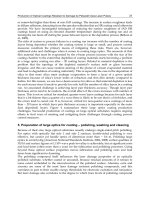
Fig. 4. All the solutions of the Parallel Robot inverse kinematics.

Differential kinematics
The following equations describe the relationship between the velocities at the joints and at
the end effector


(
)
(
)
( ) ( )
( ) ( )
1 1 1 1
1 1
1
2 2 2 2
2
2 2
3
3 3 3 3
3 3
cos sin
sin sin
cos sin
,
sin sin
cos sin
sin sin

L L
x
y
L L
L L
q a q a
a a
q
q a q a
q
a a
q
q a q a
a a
é
ù
+ +
ê ú
ê ú
é ù
ê ú
ê ú
+ +
é ù
ê ú
ê ú
= = =
ê ú
ê ú
ê ú

ë û
ê ú
ê ú
ë û
+ +
ê ú
ê ú
ê
ú
ë
û
a
q SX







(11)

1
1
2 2
1 1
1
2
2
2

2 2
2 2
3
3
3
2 2
3 3
sin sin
.
sin sin
sin sin
y
x
y
x
y
x
d
d
L L
d
d
x
y
L L
d
d
L L
a a
a

a
a a
a
a a
é
ù
ê ú
- -
ê ú
ê ú
é ù
é ù
ê ú
ê ú
= =- - =
ê ú
ê ú
ê ú
ë û
ê ú
ê ú
ë û
ê ú
ê ú
- -
ê ú
ë
û
p
q HX








(12)

(
)
( )
cos cos , 1,2,3.
sin sin , 1,2,3.
x
y
i i i i
i i i i
d L i
d L i
q q a
q q a
é
ù
= + + =
ë û
é ù
= + + =
ë
û

(13)

Concatenating (11) and (12) yields


é
ù
é
ù
= = =
ê ú
ê ú
ê
ú
ê
ú
ë
û
ë
û

 


a
p
q
S
q X WX
q

H
(14)

2.2 Dynamics of redundant planar parallel robot
In accordance with (Cheng et al., 2003), the Lagrange-D’Alembert formulation yields a
simple scheme for computing the dynamics of redundantly actuated parallel manipulators;
this approach uses the equivalent open-chain mechanism of the robot shown in Fig. 5. In
order to apply this scheme, the first step is to obtain a relationship between the joint torques
associated to all the robot joints and the robot active joint torques. The following Proposition
gives a method for obtaining this relationship


Fig. 5. Equivalent open-chain representation for the Parallel Robot.

Proposition 1: Let the joint torque Î 
n
τ of the equivalent open-chain system and the joint
torque
a
τ
of the redundantly actuated closed-chain system required to generate the same
motion; then, both torques are related as follows


.
T T
=
a
S τ W τ (15)

Proof of Proposition 1: We denote by
e
q the vector of independent generalized coordinates of
the mechanism. In the case of redundant actuation, the virtual displacement
¶
a
q of the
actuated joints is constrained. Using the kinematic constrains allows expressing
a
q
and
p
q as


(
)
(
)
= =and .
a a e p p e
q q q q q q (16)


PID Control, Implementation and Tuning34
Differentiating the above equations gives


and .d d d d
ả

ả
= =
ả ả
p
a
a e p e
e e
q
q
q q q q
q q
(17)

Applying the above results to the Lagrange-DAlembert equations yields


T T T
T
d L L d L L d L L
dt dt dt
d L L d L L
dt dt
d d d
ổ ử ổ ử ổ ử
ổ ử ổ ử ổ ử
ả ả ả ả ả ả
ữ ữ ữ
ữ ữ ữ
ỗ ỗ ỗ
ỗ ỗ ỗ

- - = - - + - -
ữ ữ ữ
ữ ữ ữ
ỗ ỗ ỗ
ỗ ỗ ỗ
ữ ữ
ỗ ỗ
ữ ữ
ỗ ỗ
ữ
ỗ
ữ
ỗ
ả ả ả ả ả ả
ố ứ ố ứ
ố ứ ố ứ
ố ứ
ố ứ
ả
ổ ử ổ
ổ ử ổ ử
ả ả ả ả
ữ
ữ ữ
ỗ
ỗ ỗ
= - - + - -
ữ
ữ ữ
ỗ

ỗ ỗ
ữ
ỗ
ữ
ỗ
ữ
ỗ
ả ả ả ả ả
ố ứ
ố ứ
ố ứ
a a p p
a a p p
a
a p
a a e p p
q q q
q q q q q q
q

q q q q q


0.
T
d
ộ ự
ả
ử
ữ

ờ ỳ
ỗ
=
ữ
ỗ
ữ
ờ ỳ
ỗ
ả
ố ứ
ở ỷ
p
e
e
q
q
q
(18)

Variable
p
is the actuating torque on the passive joints. Since d
e
q is now free to vary, the
following expression follows from (18)

, 0.
T
T
T T

d L L d L L
dt dt
ộ ự
ả
ộ ự
ờ ỳ
ổ ử
ộ ự
ả
ổ ử
ả
ổ ử ổ ử
ảả ả ả ả
ờ ỳ
ờ ỳ
ữ
ỗ
ữ
ỗ
ữ ữ
ỗ ỗ
ờ ỳ
- - - + =
ữ
ữ
ỗ
ỗ ữ ữ
ờ ỳ
ờ ỳ
ỗ ỗ ữ

ữ
ả
ỗ
ữ
ỗ
ữ
ỗ
ỗ
ữ
ả ả ả ả ả ả
ố ứ
ờ ỳ
ố ứ
ố ứ
ố ứ
ờ ỳ
ở ỷ
ờ ỳ
ở ỷ
ờ ỳ
ả
ở ỷ
a
p
a
e
a p
p
a a p p e e
e

q
q
q
q

q
q q q q q q
q

(19)

Or equivalently

.
T
T T
d L L
dt
ộ ự
ả
ờ ỳ
ả
ả
ộ ự
ổ ử
ả
ả ả
ờ ỳ
ữ
ỗ

- = +
ờ ỳ
ữ
ờ ỳ
ỗ
ữ
ả
ỗ
ả ả ả ả
ố ứ
ờ ỳ
ở ỷ
ờ ỳ
ờ ỳ
ả
ở ỷ
a
p
a
e
a p
p
e e
e
q
q
q
q

q

q q q q
q

(20)
Ignoring friction at the passive joints allows setting 0=
p
. Note also that
d L L
dt
ổ ử
ả ả
ữ
ỗ
- =
ữ
ỗ
ữ
ỗ
ữ
ỗ
ả ả
ố ứ

q q

.
These facts allow writing (20) as

=
T T

a
W S (21)


ộ ự
ả
ờ ỳ
ờ ỳ
ả
ả
ờ ỳ
= =
ờ ỳ
ả
ả
ờ ỳ
ờ ỳ
ả
ờ ỳ
ở ỷ
e
q
a
q
q
e
W
q
q
p

q
e
(22)


ả
=
ả
.
a
e
q
S
q
(23)

The Euler-Lagrange's well-known formalism (Spong et al., 2005) allows modeling each of
the legs of the open-chain mechanism in Fig. 5. Assuming that the robot moves in the
horizontal plane, the following equations model the equivalent open chain mechanism

, 1,2,3
i
i
i i
i i i
i i
i
t
q q
t

a a
ộ
ự
ộ
ự ộ ự
+ + = =
ờ ỳ
ờ ỳ ờ ỳ
ờ
ỳ ờ ỳ
ờ
ỳ
ở
ỷ ở ỷ
ở
ỷ
a
p
M C N


(24)

where


(
)
b a a b a q a
l b a g b a

g b a g
b a a
ộ
ự
ộ
ự
ộ ự
ộ ự
- - +
+ +
ờ
ỳ
ờ ỳ
ờ ỳ
= = = =
ờ ỳ
+
ờ
ỳ
ờ ỳ
ờ ỳ
ở ỷ
ở ỷ
ở
ỷ
ở
ỷ

11 12 11 12
21 22
21 22
sin sin
2 cos cos
,
cos
sin 0
i i i i
i i i i i i i
i i i i i i
i i
i i i i
i i
i i
i i i
M M C C
M M
C C
M C

(
)
l b g= + + + + = = +
2 2 2 2
1 1 1 2 2 2 2 2 2 2 2
, ,
i i i i i i i i i i i i i i i i
m r I m a r I m a r m r I

Parameters
i
j
I ,
i
j
m and
i
j
r , , :1,2,3i j , correspond to the inertia, mass, and center of mass of
each link. Combining the equations described above gives the dynamics of the open-chain
system in the form

+ + =

Mq Cq N (25)


11 12
11 12
11 12
11 12
11 12 11 12
12 22
21
12 22
21
12 22
21
1 1

1 1
2 2
2 2
1
3 3 3 3
2
1 1
1
3
2 2
2
3 3
3
0 0 0 0
0 0 0 0
0 0 0 0
0 0 0 0
0 0 0 0 0 0 0 0
, ,
0 0 0 0
0 0 0 0 0
0 0 0 0
0 0 0 0 0
0 0 0 0
0 0 0 0 0
C C
M M
C C
M M
M M C C

M M
C
M M
C
M M
C
ộ
ự
ộ ự
ờ ỳ
ờ ỳ
ờ ỳ
ờ ỳ
ộ ự
ờ ỳ
ờ ỳ
ờ
ờ ỳ
ờ ỳ
= = =
ờ
ờ ỳ
ờ ỳ
ờ
ờ ỳ
ờ ỳ
ờ
ở
ờ ỳ
ờ ỳ

ờ ỳ
ờ ỳ
ờ ỳ
ờ ỳ
ở ỷ
ở
ỷ
N
M C N N
N
ỳ
ỳ
ỳ
ỳ
ỷ
,

1 1 2 2 3 3
T






a p a p a p


The term
M is the inertial matrix, C the Coriolis and centrifugal force terms, and N is a

constant disturbance vector. The number of active and passive joints is
,n
[
]
q q q= ẻ
1 2 3
T
m
a
q stands for the active joints and
[ ]
a a a
-
= ẻ
1 2 3
T
n m
p
q for the angles of
the passive joints. In the same way, vectors
[
]
t t t= ẻ
1 2 3
,
T
m
a a a a

[

]
t t t
-
= ẻ
1 2 3
T
n m
p p p p

correspond to the torques in the active and passive joints respectively. It is worth noting
that in most parallel robots the angles of the active joints cannot play the role of generalized
coordinates because their Forward Kinematics do not have a closed form solution.,
Therefore, it is not possible to write down the dynamic equations in terms of the active
joints. For that reason, the development of the parallel robot dynamic model will consider
the robot end-effector coordinates as a set of generalized coordinates, i.e.
=
e
q X .
Substituting
in (25) into(21), we have


(
)
+ + =

.
T T
a
W Mq Cq N S (26)

Taking the time derivative of (14) leads to

= +
q WX WX



(27)

Stable Visual PID Control of Redundant Planar Parallel Robots 35
Differentiating the above equations gives


and .d d d d
ả
ả
= =
ả ả
p
a
a e p e
e e
q
q
q q q q
q q
(17)

Applying the above results to the Lagrange-DAlembert equations yields

T T T
T
d L L d L L d L L
dt dt dt
d L L d L L
dt dt
d d d
ổ ử ổ ử ổ ử
ổ ử ổ ử ổ ử
ả ả ả ả ả ả
ữ ữ ữ
ữ ữ ữ
ỗ ỗ ỗ
ỗ ỗ ỗ
- - = - - + - -
ữ ữ ữ
ữ ữ ữ
ỗ ỗ ỗ
ỗ ỗ ỗ
ữ ữ
ỗ ỗ
ữ ữ
ỗ ỗ
ữ
ỗ
ữ
ỗ
ả ả ả ả ả ả

ố ứ ố ứ
ố ứ ố ứ
ố ứ
ố ứ
ả
ổ ử ổ
ổ ử ổ ử
ả ả ả ả
ữ
ữ ữ
ỗ
ỗ ỗ
= - - + - -
ữ
ữ ữ
ỗ
ỗ ỗ
ữ
ỗ
ữ
ỗ
ữ
ỗ
ả ả ả ả ả
ố ứ
ố ứ
ố ứ
a a p p
a a p p
a

a p
a a e p p
q q q
q q q q q q
q

q q q q q


0.
T
d
ộ ự
ả
ử
ữ
ờ ỳ
ỗ
=
ữ
ỗ
ữ
ờ ỳ
ỗ
ả
ố ứ
ở
ỷ
p
e

e
q
q
q
(18)

Variable
p
is the actuating torque on the passive joints. Since d
e
q is now free to vary, the
following expression follows from (18)

, 0.
T
T
T T
d L L d L L
dt dt
ộ
ự
ả
ộ ự
ờ ỳ
ổ ử
ộ ự
ả
ổ ử
ả
ổ ử ổ ử

ảả ả ả ả
ờ ỳ
ờ ỳ
ữ
ỗ
ữ
ỗ
ữ ữ
ỗ ỗ
ờ ỳ
- - - + =
ữ
ữ
ỗ
ỗ ữ ữ
ờ ỳ
ờ ỳ
ỗ ỗ ữ
ữ
ả
ỗ
ữ
ỗ
ữ
ỗ
ỗ
ữ
ả ả ả ả ả ả
ố ứ
ờ ỳ

ố ứ
ố ứ
ố ứ
ờ ỳ
ở ỷ
ờ ỳ
ở ỷ
ờ ỳ
ả
ở
ỷ
a
p
a
e
a p
p
a a p p e e
e
q
q
q
q

q
q q q q q q
q

(19)

Or equivalently

.
T
T T
d L L
dt
ộ
ự
ả
ờ ỳ
ả
ả
ộ ự
ổ ử
ả
ả ả
ờ ỳ
ữ
ỗ
- = +
ờ ỳ
ữ
ờ ỳ
ỗ
ữ
ả
ỗ
ả ả ả ả
ố ứ

ờ ỳ
ở ỷ
ờ ỳ
ờ ỳ
ả
ở
ỷ
a
p
a
e
a p
p
e e
e
q
q
q
q

q
q q q q
q

(20)
Ignoring friction at the passive joints allows setting 0=
p
. Note also that
d L L
dt

ổ ử
ả ả
ữ
ỗ
- =
ữ
ỗ
ữ
ỗ
ữ
ỗ
ả ả
ố ứ

q q

.
These facts allow writing (20) as

=
T T
a
W S (21)


ộ
ự
ả
ờ ỳ
ờ ỳ

ả
ả
ờ ỳ
= =
ờ ỳ
ả
ả
ờ ỳ
ờ ỳ
ả
ờ ỳ
ở
ỷ
e
q
a
q
q
e
W
q
q
p
q
e
(22)


ả
=

ả
.
a
e
q
S
q
(23)

The Euler-Lagrange's well-known formalism (Spong et al., 2005) allows modeling each of
the legs of the open-chain mechanism in Fig. 5. Assuming that the robot moves in the
horizontal plane, the following equations model the equivalent open chain mechanism

, 1,2,3
i
i
i i
i i i
i i
i
t
q q
t
a a
ộ ự
ộ ự ộ ự
+ + = =
ờ ỳ
ờ ỳ ờ ỳ
ờ ỳ ờ ỳ

ờ ỳ
ở ỷ ở ỷ
ở ỷ
a
p
M C N


(24)

where


(
)
b a a b a q a
l b a g b a
g b a g
b a a
ộ ự
ộ ự
ộ ự
ộ ự
- - +
+ +
ờ ỳ
ờ ỳ
ờ ỳ
= = = =
ờ ỳ

+
ờ ỳ
ờ ỳ
ờ ỳ
ở ỷ
ở ỷ
ở ỷ
ở ỷ



11 12 11 12
21 22
21 22
sin sin
2 cos cos
,
cos
sin 0
i i i i
i i i i i i i
i i i i i i
i i
i i i i
i i
i i
i i i
M M C C
M M
C C

M C

( )
l b g= + + + + = = +
2 2 2 2
1 1 1 2 2 2 2 2 2 2 2
, ,
i i i i i i i i i i i i i i i i
m r I m a r I m a r m r I

Parameters
i
j
I ,
i
j
m and
i
j
r , , :1,2,3i j , correspond to the inertia, mass, and center of mass of
each link. Combining the equations described above gives the dynamics of the open-chain
system in the form


+ + =

Mq Cq N (25)


11 12

11 12
11 12
11 12
11 12 11 12
12 22
21
12 22
21
12 22
21
1 1
1 1
2 2
2 2
1
3 3 3 3
2
1 1
1
3
2 2
2
3 3
3
0 0 0 0
0 0 0 0
0 0 0 0
0 0 0 0
0 0 0 0 0 0 0 0
, ,

0 0 0 0
0 0 0 0 0
0 0 0 0
0 0 0 0 0
0 0 0 0
0 0 0 0 0
C C
M M
C C
M M
M M C C
M M
C
M M
C
M M
C
ộ ự
ộ ự
ờ ỳ
ờ ỳ
ờ ỳ
ờ ỳ
ộ ự
ờ ỳ
ờ ỳ
ờ
ờ ỳ
ờ ỳ
= = =

ờ
ờ ỳ
ờ ỳ
ờ
ờ ỳ
ờ ỳ
ờ
ở
ờ ỳ
ờ ỳ
ờ ỳ
ờ ỳ
ờ ỳ
ờ ỳ
ở ỷ
ở ỷ
N
M C N N
N
ỳ
ỳ
ỳ
ỳ
ỷ
,

1 1 2 2 3 3
T

a p a p a p


The term
M is the inertial matrix, C the Coriolis and centrifugal force terms, and N is a
constant disturbance vector. The number of active and passive joints is
,n
[ ]
q q q= ẻ
1 2 3
T
m
a
q stands for the active joints and
[ ]
a a a
-
= ẻ
1 2 3
T
n m
p
q for the angles of
the passive joints. In the same way, vectors
[
]
t t t= ẻ
1 2 3

,
T
m
a a a a

[ ]
t t t
-
= ẻ
1 2 3
T
n m
p p p p

correspond to the torques in the active and passive joints respectively. It is worth noting
that in most parallel robots the angles of the active joints cannot play the role of generalized
coordinates because their Forward Kinematics do not have a closed form solution.,
Therefore, it is not possible to write down the dynamic equations in terms of the active
joints. For that reason, the development of the parallel robot dynamic model will consider
the robot end-effector coordinates as a set of generalized coordinates, i.e.
=
e
q X .
Substituting
in (25) into(21), we have


(
)
+ + =

.
T T
a
W Mq Cq N S (26)

Taking the time derivative of (14) leads to

= +
q WX WX



(27)

PID Control, Implementation and Tuning36
Substituting q

and q

given in(14) and (27) into (26) produces the following dynamic model

,
T
+ + =
a
MX CX N S τ
 
(28)
where

,
,
.
T
T T
T
=
= +
=
M W MW
C W MW W CW
N W N






Note that the above model relates the active joint torques
a
τ
and the end–effector
coordinates
X . The inertia matrix M and the Coriolis matrix C satisfy the following
structural properties as long as matrix
W
has full rank

Property 1. Matrix M is a symmetric and positive definite.

Property 2. Matrix 2-M C

is skew-symmetric.

Property 3. There exists a positive constant
1C
k such that


£

1
.k
C
C X (29)

3. Model of the vision system
Consider the redundant planar parallel robot described previously together with its
Cartesian coordinate frame
x y-
R R
(see Fig. 6). This coordinate frame defines a plane where
the motion of the robot end-effector takes place. A camera providing an image of the whole
robot workspace, including the robot end-effector, is perpendicular to the plane where the
robot evolves. The optical center is located at a distance
z with respect to the
-x y
R R

plane,
and the intersection
[ ]
T
x y
O OO  between the optical axis and the robot workspace is
located anywhere in the robot workspace. Variable

denotes the orientation of the camera
around the optical axis with respect to the negative side of axis x
R
of the robot coordinate
frame, measured clockwise.
The camera sensor has associated a coordinate frame called the image coordinate frame with
axes
i
x and
i
y ; they are parallel to the robot coordinate frame. The camera sensor captures
the image that is later stored in the computer frame buffer and displayed in the computer
screen. The visual feature of interest is the robot end-effector position
=[ ]
T
i i
x y
i
X
defined in
the image coordinate frame; the units for
i

X are pixels. Image-processing algorithms, allow
the estimation of the coordinate
i
X
. Thus, this estimate feeds the control algorithm without
further processing. This later feature is common to all image-based Visual Servoing
algorithms and permits avoiding camera calibration procedures.


Fig. 6. Fixed-camera robotic system, robot and camera coordinate frames.

Let assume a perspective transformation as an ideal pinhole camera model (Kelly, 1996), the
next relationship describes the position of the end-effector given in the image coordinate
frame in terms of its position in the robot workspace


(
)
h b= - +( )h
i i
X R X O C (30)

Parameter
[
]
=
T
x y
C C
i i i

C is the image center,
h
is a scale factor in pixels/m, which is assumed
negative, h is the magnification factor defined as


l
l
= <
-
0h
z
(31)

where l is the camera focal distance.
( ) (2)SOR


is the rotation matrix generated by
clockwise rotating the camera about its optical axis by

radians


cos sin
( ) .
sin cos
R














(32)

The time derivative of (30) gives the end-effector linear velocity in terms of the image
coordinate frame


h b=
 
( ) .h
i
X R X
(33)

Stable Visual PID Control of Redundant Planar Parallel Robots 37
Substituting q

and q

given in(14) and (27) into (26) produces the following dynamic model

,
T
+ + =
a
MX CX N S τ
 
(28)
where

,
,
.
T
T T
T
=
= +
=
M W MW
C W MW W CW
N W N






Note that the above model relates the active joint torques
a

τ
and the end–effector
coordinates
X . The inertia matrix M and the Coriolis matrix C satisfy the following
structural properties as long as matrix
W
has full rank


Property 1. Matrix M is a symmetric and positive definite.

Property 2. Matrix 2-M C

is skew-symmetric.

Property 3. There exists a positive constant
1C
k such that


£

1
.k
C
C X (29)

3. Model of the vision system
Consider the redundant planar parallel robot described previously together with its
Cartesian coordinate frame

x y-
R R
(see Fig. 6). This coordinate frame defines a plane where
the motion of the robot end-effector takes place. A camera providing an image of the whole
robot workspace, including the robot end-effector, is perpendicular to the plane where the
robot evolves. The optical center is located at a distance
z with respect to the
-x y
R R
plane,
and the intersection
[ ]
T
x y
O OO  between the optical axis and the robot workspace is
located anywhere in the robot workspace. Variable

denotes the orientation of the camera
around the optical axis with respect to the negative side of axis x
R
of the robot coordinate
frame, measured clockwise.
The camera sensor has associated a coordinate frame called the image coordinate frame with
axes
i
x and
i
y ; they are parallel to the robot coordinate frame. The camera sensor captures
the image that is later stored in the computer frame buffer and displayed in the computer
screen. The visual feature of interest is the robot end-effector position

=[ ]
T
i i
x y
i
X
defined in
the image coordinate frame; the units for
i
X are pixels. Image-processing algorithms, allow
the estimation of the coordinate
i
X
. Thus, this estimate feeds the control algorithm without
further processing. This later feature is common to all image-based Visual Servoing
algorithms and permits avoiding camera calibration procedures.


Fig. 6. Fixed-camera robotic system, robot and camera coordinate frames.

Let assume a perspective transformation as an ideal pinhole camera model (Kelly, 1996), the
next relationship describes the position of the end-effector given in the image coordinate
frame in terms of its position in the robot workspace


(
)
h b= - +( )h
i i
X R X O C (30)

Parameter
[ ]
=
T
x y
C C
i i i
C is the image center,
h
is a scale factor in pixels/m, which is assumed
negative, h is the magnification factor defined as


l
l
= <
-
0h
z
(31)

where l is the camera focal distance.
( ) (2)SOR

 is the rotation matrix generated by
clockwise rotating the camera about its optical axis by

radians

cos sin
( ) .
sin cos
R
 




 

 
 
(32)

The time derivative of (30) gives the end-effector linear velocity in terms of the image
coordinate frame


h b=
 
( ) .h
i
X R X
(33)

PID Control, Implementation and Tuning38
The following equation gives the desired end-effector position
[ ]

=
* *
T
x y
*
X expressed in
terms of the image coordinate frame


(
)
h b= - +( )h
* *
i i
X R X O C
(34)

where
[ ]
=
* *
T
x y
*
X denotes the desired end-effector position expressed in the robot
coordinate frame and located strictly inside the robot workspace, so there exists at least one
(unknown) constant joint position vector, say
6
Î
d

q  for which the robot end-effector
reaches the desired position, in other words, there exists a nonempty set
Ì
n
Q such that
( )f
= ÎW
*
da
X q for QÎ
da
q . At this point, it is convenient to introduce the definition of the
image position error

i
X as the visual distance between the measured and desired end-
effector positions, see Fig. 7, i.e.


é ù
é ù
= - = -
ê ú
ê ú
ê ú
ë û
ë û

.
x x

y
y
*
*
i i
*
i i i
i
i
X X X
(35)

Therefore, expressions (30),(34), and (35) allow defining the image error vector

i
X as


[
]
( ) ( ) ( ) .hh b j j= -
i da a
X R q q

(36)

Assuming a fixed desired position, taking the time derivative of the image position error
yields

( ) .
d
h
dt
h b=- =-
i
i
X
X R X

 
(37)

4. Visual PID control algorithm
4.1 Preliminaries
A standard linear PID control law has the following form


0
( )
t
P I D
u K e K e d K es s= + +
ò

(38)

Here, variable e r
y
= - defines the error with r the set point and

y
the output variable;
therefore, the error
e
as well as its time-integral and time-derivative feed this algorithm. In
some cases, the time derivative
y
-

replaces e

leading to the controller


0
( )
t
P I D
u K e K e d K
y
s s= + -
ò

(39)


Fig. 7. Image position error in the image coordinate frame.

This last controller attenuates overshoots in face of abrupt changes in the set point value.
When applied to joint control of robot manipulators, the linear PID controller leads to local

stability or semi-global stability results. Applying a saturating function to the error, the
Authors in references (Kelly, 1998) and (Santibañez & Kelly, 1998) were able to obtain global
stability results. The next expression is an example of a PID controller using saturating
functions

0
( ( )) .
t
P I D
u K e K
f
e d K
y
s s= + -
ò

(40)

In this case, the term
( )
f
⋅ corresponds to a saturation function applied to the error. The
proposed method for the control the redundant parallel robot will resort on a similar
approach. The following definition states some key properties of the saturating functions
used in the control law described in subsequent paragraphs.

Definition 1.  e( , , )m x with 1 0m³ > , 0e> and Î
n
x denotes the set of all continuous
differentiable increasing functions

[
]
= 
1 2
( ) ( ) ( ) ( )
T
n
f f x f x f xx such that


( ) , : ;x f x m x x x e³ ³ " Î <

 ( ) , : ;f x m x xe e e³ ³ " Î ³
 1 ( / ) ( ) 0;d dx f x³ ³

where
⋅ stands for the absolute value.

Stable Visual PID Control of Redundant Planar Parallel Robots 39
The following equation gives the desired end-effector position
[ ]
=
* *
T
x y
*
X expressed in
terms of the image coordinate frame

(
)
h b= - +( )h
* *
i i
X R X O C
(34)

where
[ ]
=
* *
T
x y
*
X denotes the desired end-effector position expressed in the robot
coordinate frame and located strictly inside the robot workspace, so there exists at least one
(unknown) constant joint position vector, say
6
Î
d
q  for which the robot end-effector
reaches the desired position, in other words, there exists a nonempty set
Ì
n
Q such that
( )f
= ÎW
*
da

X q for QÎ
da
q . At this point, it is convenient to introduce the definition of the
image position error

i
X as the visual distance between the measured and desired end-
effector positions, see Fig. 7, i.e.


é
ù
é
ù
= - = -
ê ú
ê
ú
ê
ú
ë
û
ë
û

.
x x
y
y
*

*
i i
*
i i i
i
i
X X X
(35)

Therefore, expressions (30),(34), and (35) allow defining the image error vector

i
X as


[
]
( ) ( ) ( ) .hh b j j= -
i da a
X R q q

(36)

Assuming a fixed desired position, taking the time derivative of the image position error
yields


( ) .
d
h

dt
h b=- =-
i
i
X
X R X

 
(37)

4. Visual PID control algorithm
4.1 Preliminaries
A standard linear PID control law has the following form


0
( )
t
P I D
u K e K e d K es s= + +
ò

(38)

Here, variable e r
y
= - defines the error with r the set point and
y
the output variable;
therefore, the error

e
as well as its time-integral and time-derivative feed this algorithm. In
some cases, the time derivative
y
-

replaces e

leading to the controller


0
( )
t
P I D
u K e K e d K
y
s s= + -
ò

(39)


Fig. 7. Image position error in the image coordinate frame.

This last controller attenuates overshoots in face of abrupt changes in the set point value.
When applied to joint control of robot manipulators, the linear PID controller leads to local
stability or semi-global stability results. Applying a saturating function to the error, the
Authors in references (Kelly, 1998) and (Santibañez & Kelly, 1998) were able to obtain global
stability results. The next expression is an example of a PID controller using saturating

functions

0
( ( )) .
t
P I D
u K e K
f
e d K
y
s s= + -
ò

(40)

In this case, the term
( )
f
⋅ corresponds to a saturation function applied to the error. The
proposed method for the control the redundant parallel robot will resort on a similar
approach. The following definition states some key properties of the saturating functions
used in the control law described in subsequent paragraphs.

Definition 1.  e( , , )m x with 1 0m³ > , 0e> and Î
n
x denotes the set of all continuous
differentiable increasing functions
[ ]
= 
1 2

( ) ( ) ( ) ( )
T
n
f f x f x f xx such that


( ) , : ;x f x m x x x e³ ³ " Î <

 ( ) , : ;f x m x xe e e³ ³ " Î ³
 1 ( / ) ( ) 0;d dx f x³ ³

where
⋅ stands for the absolute value.

PID Control, Implementation and Tuning40
Figure 8 depicts the region allowed for functions belonging to the set  e( , , )m x . Two
important properties of functions
( )
f
x belonging to  e( , , )m x are now stated

Property 4. The Euclidean norm of ( ),
n
f Îx x  satisfies

,
( )
,
m if
f

m if
e
e e
ì
<
ï
ï
³
í
ï
³
ï
î
x x
x
x
,
,
( )
, .
if
f
n if
e
e e
ì
<
ï
ï
£

í
ï
³
ï
î
x x
x
x


Property 5. The function ( ) ,
T n
f Îx x x  satisfies

2
,
( )
, .
T
m if
f
m if
e
e e
ì
ï
<
ï
³
í

ï
³
ï
î
x x
x x
x x



Fig. 8. Saturating functions
 e( , , )m x .

4.2 Control problem formulation
Consider the robotic system described in Fig.6. Assume that the camera together with the
vision system provide the position
[ ]
T
x y=
i i i
X of the robot end-effector expressed in the
image coordinate frame. Suppose that measurements of joint position q and velocity
q

are
available. However, the magnification factor h and the position of the intersection of the
camera axis with the robot workspace
[ ]
T
x y

O O=O expressed in terms of the robot
coordinate frame are assumed unknown. The control problem can be stated as that of
designing a control law for the active joint actuator torques
a
τ such that the robot end-
effector reaches, in the image supplied on the screen, the desired position defined in the
robot workspace, i.e., the control law must ensure that
(
)
¥
- =lim
t
*
i i
X X 0
for
2
ÎWÌ
*
i
X  .
In order to solve the problem stated previously, assume that

.
T
=
a
S τ u (41)

Variable u defines a control signal in terms of the end-effector coordinates, and drives the

robot dynamics (28). Hence, torques
a
τ
are the solutions of the following equation


( )
†
.
T
=
a
τ S u (42)

The symbol
( ) ( )
† 1
T T
-
=S S S S stands for the Moore-Penrose pseudo-inverse of
T
S , satisfying
( )
†
T T
I=S S , and
( )
[
]
†

†
T
T T
I= =S S S S . Solution (42) makes sense only if the pseudo-inverse
( )
†
T
S
is well defined, i.e., if matrix S has full rank. Matrix S loose rank if the parallel robot
reaches a singular configuration; in the sequel, matrix S is assumed full rank. Let us propose
the following PID control law


( )
0
( )
t
f ds s= + -
ò
P I D
u K Y K Y K X

(43)

Using (41) and (42) allows writing the control law (39) as follows


( )
( )
†

0
( )
t
T
f ds s
é
ù
= + -
ê
ú
ë
û
ò
a P I D
τ S K Y K Y K X

(44)

The term b=

( )
T
i
Y R X corresponds to the rotated position error, variables
P
K ,
I
K and
D
K are

diagonal positive definite matrices and correspond to the proportional, integral and
derivative actions. The above control law is composed of a linear Proportional Derivative
(PD) term plus an integral action of the nonlinear function of the position error
( )f Y . Note
that the position error

i
X feeds the proportional and the integral actions, whereas the active
joint velocities
a
q

feed the derivative action using the relationship
†
=
a
X S q


. Note also that in
order to implement control law (44) it is not necessary to know the parameters
h and h ;
hence, camera calibration is not necessary. The Fig. 9 depicts the corresponding block
diagram.
Stable Visual PID Control of Redundant Planar Parallel Robots 41
Figure 8 depicts the region allowed for functions belonging to the set  e( , , )m x . Two
important properties of functions
( )
f
x belonging to  e( , , )m x are now stated

Property 4. The Euclidean norm of ( ),
n
f Îx x  satisfies

,
( )
,
m if
f
m if
e
e e
ì
<
ï
ï
³
í
ï
³
ï
î
x x
x
x
,
,
( )
, .

if
f
n if
e
e e
ì
<
ï
ï
£
í
ï
³
ï
î
x x
x
x


Property 5. The function ( ) ,
T n
f Îx x x  satisfies

2
,
( )
, .
T
m if

f
m if
e
e e
ì
ï
<
ï
³
í
ï
³
ï
î
x x
x x
x x



Fig. 8. Saturating functions
 e( , , )m x .

4.2 Control problem formulation
Consider the robotic system described in Fig.6. Assume that the camera together with the
vision system provide the position
[
]
T
x y=

i i i
X of the robot end-effector expressed in the
image coordinate frame. Suppose that measurements of joint position q and velocity
q

are
available. However, the magnification factor h and the position of the intersection of the
camera axis with the robot workspace
[
]
T
x y
O O=O expressed in terms of the robot
coordinate frame are assumed unknown. The control problem can be stated as that of
designing a control law for the active joint actuator torques
a
τ such that the robot end-
effector reaches, in the image supplied on the screen, the desired position defined in the
robot workspace, i.e., the control law must ensure that
(
)
¥
- =lim
t
*
i i
X X 0
for
2
ÎWÌ

*
i
X  .
In order to solve the problem stated previously, assume that

.
T
=
a
S τ u (41)

Variable u defines a control signal in terms of the end-effector coordinates, and drives the
robot dynamics (28). Hence, torques
a
τ
are the solutions of the following equation


( )
†
.
T
=
a
τ S u (42)

The symbol
( ) ( )
† 1
T T

-
=S S S S stands for the Moore-Penrose pseudo-inverse of
T
S , satisfying
( )
†
T T
I=S S , and
( )
[ ]
†
†
T
T T
I= =S S S S . Solution (42) makes sense only if the pseudo-inverse
( )
†
T
S
is well defined, i.e., if matrix S has full rank. Matrix S loose rank if the parallel robot
reaches a singular configuration; in the sequel, matrix S is assumed full rank. Let us propose
the following PID control law


( )
0
( )
t
f ds s= + -
ò

P I D
u K Y K Y K X

(43)

Using (41) and (42) allows writing the control law (39) as follows


( )
( )
†
0
( )
t
T
f ds s
é ù
= + -
ê ú
ë û
ò
a P I D
τ S K Y K Y K X

(44)

The term b=

( )
T

i
Y R X corresponds to the rotated position error, variables
P
K ,
I
K and
D
K are
diagonal positive definite matrices and correspond to the proportional, integral and
derivative actions. The above control law is composed of a linear Proportional Derivative
(PD) term plus an integral action of the nonlinear function of the position error
( )f Y . Note
that the position error

i
X feeds the proportional and the integral actions, whereas the active
joint velocities
a
q

feed the derivative action using the relationship
†
=
a
X S q


. Note also that in
order to implement control law (44) it is not necessary to know the parameters
h and h ;

hence, camera calibration is not necessary. The Fig. 9 depicts the corresponding block
diagram.
PID Control, Implementation and Tuning42

Fig. 9. Block diagram of the Visual PID control law.

Substituting control law (44) into the robot dynamics (28) and defining an auxiliary variable
Z
as

( )
1
0
( )
t
f ds s
-
= -
ò
I
Z Y K N (45)

yield the closed-loop dynamics


{ }
1
( )
h
d

dt
f
h
-
é ù
-
é ù
ê ú
ê ú
ê ú
ê ú
= + - -
ê ú
ê ú
ê ú
ê ú
ê ú
ê ú
ë û ë û
P I D
X
Y
X M K Y K Z K X CX
Z Y

  
(46)

The following proposition provides conditions on the controller gains
, ,

P D
K K and
I
K guaranteeing the asymptotic stability of the equilibrium of the closed-loop dynamics.

Proposition 2. Consider the robot dynamics (28) together with control law (44) where
Î( )f Y  ( , , )m xe . Assume that the PID controller gains fulfill


{
}
{
}
min max 2 2
, 0k kl l> + >
D C C
K M (47)

{ } { }
{ }
min max max
2
h
l l l
h
> +
P I
K K M (48)

Then, the equilibrium

[ ]
0 0 0
T
T
é ù
=
ë û
Y X Z

of (46) is asymptotically stable.


Proof of Proposition 2: The stability analysis employs the following Lyapunov Function
Candidate


( )
[ ] [ ]
[ ]
2 2
2 2
1 1 1 1 1
, , ( ) ( ) ( )
2 2
1 1
( ) ( ).
2 2
T
T
T

T T
V
f f f
w dw
h h h h
f f
h h
h h h h
h h
é ù é ù
= - - + + + +
ê ú ê ú
ê ú ê ú
ë û ë û
+ - -
ò
Y
I D
0
P I
Y X Z X Y M X Y Z Y K Z Y K
Y K K Y Y M Y
  
(49)

The first term is a nonnegative function of
Y and X

, while the second is a nonnegative
function of variables

Y and Z . Using the fact that
D
K is a diagonal positive definite
matrix,
( )f =0 0
, and the entries of
( )f Y
are increasing functions, it is not difficult to show
that the third term satisfies


2 2
1
( ) 0, 0
T
f w dw
h
h
> " ¹
ò
Y
D
0
K Y (50)

Therefore, this term is positive definite with respect to
Y . For the remaining terms, notice
that using the Rayleigh-Ritz inequality leads to

[ ] { } { }
{ }
2 2
min max max
2 2 2 2
1 1 1 1
( ) ( ) ( ) .
2 2 2 2
T T
f f f
h h h h
l l l
h h h h
é ù
- - ³ - -
ë û
P I P I
Y K K Y Y M Y K K Y M Y

The above result and Property 4 yields

{ } { }
{ }
{ } { }
{ }
{ } { }
{ }
2
min max max
2 2

min max max
2 2
2
min max max
1 1
,
1 1
2
( )
1 2
2 2
, .
2
if
h h
f
h h
if
h h
l l l e
h h
l l l
h h
l l l e e
h h
ì
é
ù
ï
ï

ê ú
- - <
ï
ï
ê ú
ï
ë û
é ù
- - ³
í
ë û
é ù
ï
ï
ê ú
- - ³
ï
ê ú
ï
ë
ûï
î
P I
P I
P I
K K M Y Y
K K Y M Y
K K M Y
(51)

The right-hand side of (51) is a positive definite function with respect to
Y because of
inequality (48); therefore, the Lyapunov function candidate (49) is a positive definite
function. The following equation gives the time derivative of Lyapunov Function Candidate
(49)


( )
2 2 2 2
2 2
2 2
1 1 1 1 1 1
, , ( ) ( ) ( ) ( ) ( ) ( ) ( )
2 2
1 1 1 1 1 1 1
( )
1
(
T T T T T T T
T T T T T T T
d
V f f f f f f f
dt h h h h h
d
f w dw
h h h h dt h h h
f
h
h h h h h
h h h h h h h

h
= - - + + - +
é ù
ê ú
+ + + + + + -
ê ú
ë û
-
ò
Y
I I I I D P I
0
Y X Z X MX X M Y Y MX Y M Y X MX Y MX Y M Y
Z K Z Z K Y Y K Z Y K Y K Y K Y Y K Y
Y
 
       
  
   
 
2 2
1
) ( ) ( ) ( ).
2
T T
f f f
hh
-M Y Y M Y



Applying the Leibnitz rule to the time derivative of the integral term produces


2 2 2 2
1 1
( ) ( ) .
T T
d
f w dw f
dt h h
h h
é
ù
ê ú
=
ê ú
ë
û
ò
Y
D D
0
K Y K Y



From the above, the Lyapunov Functions Candidate time derivative becomes
Stable Visual PID Control of Redundant Planar Parallel Robots 43

Fig. 9. Block diagram of the Visual PID control law.

Substituting control law (44) into the robot dynamics (28) and defining an auxiliary variable
Z
as

( )
1
0
( )
t
f ds s
-
= -
ò
I
Z Y K N (45)

yield the closed-loop dynamics


{ }
1
( )
h
d
dt
f
h

-
é
ù
-
é ù
ê
ú
ê ú
ê
ú
ê ú
= + - -
ê
ú
ê ú
ê
ú
ê ú
ê
ú
ê
ú
ë
û ë û
P I D
X
Y
X M K Y K Z K X CX
Z Y


  
(46)

The following proposition provides conditions on the controller gains
, ,
P D
K K and
I
K guaranteeing the asymptotic stability of the equilibrium of the closed-loop dynamics.

Proposition 2. Consider the robot dynamics (28) together with control law (44) where
Î( )f Y  ( , , )m xe . Assume that the PID controller gains fulfill


{
}
{
}
min max 2 2
, 0k kl l> + >
D C C
K M (47)

{ } { }
{ }
min max max
2
h
l l l
h

> +
P I
K K M (48)

Then, the equilibrium
[ ]
0 0 0
T
T
é ù
=
ë
û
Y X Z

of (46) is asymptotically stable.


Proof of Proposition 2: The stability analysis employs the following Lyapunov Function
Candidate


( )
[ ] [ ]
[ ]
2 2
2 2
1 1 1 1 1
, , ( ) ( ) ( )
2 2

1 1
( ) ( ).
2 2
T
T
T
T T
V
f f f
w dw
h h h h
f f
h h
h h h h
h h
é ù é ù
= - - + + + +
ê ú ê ú
ê ú ê ú
ë û ë û
+ - -
ò
Y
I D
0
P I
Y X Z X Y M X Y Z Y K Z Y K
Y K K Y Y M Y
  
(49)

The first term is a nonnegative function of
Y and X

, while the second is a nonnegative
function of variables
Y and Z . Using the fact that
D
K is a diagonal positive definite
matrix,
( )f =0 0
, and the entries of
( )f Y
are increasing functions, it is not difficult to show
that the third term satisfies


2 2
1
( ) 0, 0
T
f w dw
h
h
> " ¹
ò
Y
D
0
K Y (50)

Therefore, this term is positive definite with respect to
Y . For the remaining terms, notice
that using the Rayleigh-Ritz inequality leads to


[ ] { } { }
{ }
2 2
min max max
2 2 2 2
1 1 1 1
( ) ( ) ( ) .
2 2 2 2
T T
f f f
h h h h
l l l
h h h h
é ù
- - ³ - -
ë û
P I P I
Y K K Y Y M Y K K Y M Y

The above result and Property 4 yields

{ } { }
{ }
{ } { }

{ }
{ } { }
{ }
2
min max max
2 2
min max max
2 2
2
min max max
1 1
,
1 1
2
( )
1 2
2 2
, .
2
if
h h
f
h h
if
h h
l l l e
h h
l l l
h h
l l l e e

h h
ì
é ù
ï
ï
ê ú
- - <
ï
ï
ê ú
ï
ë û
é ù
- - ³
í
ë û
é ù
ï
ï
ê ú
- - ³
ï
ê ú
ï
ë ûï
î
P I
P I
P I
K K M Y Y

K K Y M Y
K K M Y
(51)

The right-hand side of (51) is a positive definite function with respect to
Y because of
inequality (48); therefore, the Lyapunov function candidate (49) is a positive definite
function. The following equation gives the time derivative of Lyapunov Function Candidate
(49)


( )
2 2 2 2
2 2
2 2
1 1 1 1 1 1
, , ( ) ( ) ( ) ( ) ( ) ( ) ( )
2 2
1 1 1 1 1 1 1
( )
1
(
T T T T T T T
T T T T T T T
d
V f f f f f f f
dt h h h h h
d
f w dw
h h h h dt h h h

f
h
h h h h h
h h h h h h h
h
= - - + + - +
é ù
ê ú
+ + + + + + -
ê ú
ë û
-
ò
Y
I I I I D P I
0
Y X Z X MX X M Y Y MX Y M Y X MX Y MX Y M Y
Z K Z Z K Y Y K Z Y K Y K Y K Y Y K Y
Y
 
       
  
   
 
2 2
1
) ( ) ( ) ( ).
2
T T
f f f

hh
-M Y Y M Y




Applying the Leibnitz rule to the time derivative of the integral term produces


2 2 2 2
1 1
( ) ( ) .
T T
d
f w dw f
dt h h
h h
é ù
ê ú
=
ê ú
ë û
ò
Y
D D
0
K Y K Y


From the above, the Lyapunov Functions Candidate time derivative becomes
PID Control, Implementation and Tuning44
( )
2 2
1 1 1 1
, , ( ) ( ) ( )
2
1 1 1 1 1 1 1
( )
T T T T T
T T T T T T T
d
V f f f
dt h h h
f
h h h h h h h
h h h
h h h h h h h
= - - + -
+ + + + + + -
I I I I D P I
Y X Z X MX X M Y Y MX X MX Y MX
Z K Z Z K Y Y K Z Y K Y Y K Y Y K Y Y K Y

       
 
    
 
(52)

Note that the time derivative of the saturating function
( )f Y fulfills ( ) ( )f hFh=-Y Y X


. The
term
( )F Y is a diagonal matrix, and its entries ( )/ ; 1,2
j j
f j¶ ¶ =Y Y are nonnegative and
smaller than or equal to one. Substituting the closed-loop dynamics (46) into (52) yields

( )
, , ( )
1 1 1 1 1 1
( ) ( ) ( ) ( ) ( )
2
1 1 1
( ) ( ) ( ) .
T T T T T
T T T T T T
T T T T T T T
d
V F
dt
f f f f f
h h h h h
f f f
h h h
h h h h h
h h h

= + - - +
- - + + + -
+ - + - - - +
P I D
P I D
I I I I D P I
Y X Z X K Y X K Z X K X X CX X M Y X
Y K Y Y K Z Y K X Y CX X MX Y MX
Z K Y Z K X Y K Y Y K X Y K X Y K X Y K X
        
    
 
    


Some simplifications and the use of
Property 2 lead to the following expression for the time
derivative of the Lyapunov Function Candidate (49) along the trajectories of the closed-loop
system (46)


( )
[ ]
[ ]
h h
=- - - - -
   

1 1
, , ( ) ( ) ( )

T T T T
V F f f
h h
D P I
Y X Z X K M Y X Y K K Y Y C X (53)

By using
Properties 3 and 4 we have


2 2
1 2
1 1
( ) 2 .
T T
f k k
h h
e
h h
- £ =
C C
Y C X X X
  


On the other hand, note that


{ }
2

max
( ) .
T
F l£X M Y X M X
  


Therefore, the time derivative of the Lyapunov Function Candidate (53) satisfies


( )
[ ]
2
1
, , ( )
T
V f
h
g
h
£- - -
P I
Y X Z X Y K K Y
 

(54)

The parameter
{
}

{
}
min max 2
kg l l= - -
D C
K M is positive because of the selection of
D
K in (47).
The fact that
P
K and
I
K are diagonal positive definite matrices and ( ) 0
i i
f ³Y Y allows
establishing the following upper bound for the second term of (54)


[ ] { } { }
[ ]
min max
1 1
( ) ( ) .l l
h h
- - £- -
P I P I
Y K K Y K K Y Y
T T
f f
h h

Taking into account Property 5 leads to


[ ]
2
1
,
( )
,
T
if
f
if
h
m e
me e
h
ì
ï
- <
ï
- - £
í
ï
- ³
ï
î
P I

Y Y
Y K K Y
Y Y
(55)

The choice of
P
K
in (48) ensures
{ } { }
[ ]
min max
0
m
h
m l l
h
= - >
P I
K K .
Therefore, incorporating (55) into(54) produces the following a negative semi-definite
function

( )
2
2
2
,
, ,
,

if
V
if
g m e
g me e
ì
ï
- - <
ï
ï
£
í
ï
- - ³
ï
ï
î
X Y Y
Y X Z
X Y Y




(56)

Using the fact that the Lyapunov Function Candidate (49) is a positive definite function and
its time derivative is a negative semi-definite function, allows concluding that the
equilibrium of the closed-loop system (46) is stable. Finally, by invoking the LaSalle’s
invariance principle permits establishing asymptotical stability as follows. Since

(
)
, , 0V ºY X Z


if and only if X

and Y are zero. This implies that X

, Y

, and ( )
f
Y are also
zero; then, from the closed-loop system (46) , it follows that
{
}
1-
+ - - =
P I D
M K Y K Z K X CX 0
 
.
This result allows concluding
0=
I
K Z
. Therefore, 0=Z because
I
K

is a diagonal positive
definite matrix. Thus,
(
)
, , 0V ºY X Z


in the invariant set
{
}
, ,= = =Y 0 X 0 Z 0

and asymptotic
stability follows.

Some comments regarding the proposed control law are worth making. Firstly, note that the
measurements provided by the vision system feed the integral and proportional actions. The
Derivative action employs velocity measurements from the active joints; then, using the
relationship
†
=
a
X S q


allows obtaining velocity estimates of the robot end effector. In
practice, since in most cases, the robot active joints are endowed only with position sensors,
high-pass filter or backward differences approaches would permit estimating
a
q


from
position measurements. An advantage of using
a
q

for generating the Derivative action is
that position measurements at the active joints, supplied in most cases by optical encoders,
are obtained at higher sampling rates compared with the measurements provided by a
vision system. The reader will note in the next section that the sampling rate for the
incremental optical encoders associated to the active joints is five times faster than that
corresponding to the measurements obtained though the vision system.

5. Experimental Results
Experiments conducted on a laboratory prototype (Fig. 10) display the performance of the
proposed controller. The nominal link lengths of the prototype are
15L cm= . Brushed servomotors
from Moog, model C34L80W40 drive the active joints. Incremental optical encoders attached to the
motors provide position measurements corresponding to the vector
a
q . These motors steer the active
joints through timing belts with a 3.6:1 ratio. Pulse width modulation digital amplifiers from Copley
Stable Visual PID Control of Redundant Planar Parallel Robots 45
( )
2 2
1 1 1 1
, , ( ) ( ) ( )
2
1 1 1 1 1 1 1
( )

T T T T T
T T T T T T T
d
V f f f
dt h h h
f
h h h h h h h
h h h
h h h h h h h
= - - + -
+ + + + + + -
I I I I D P I
Y X Z X MX X M Y Y MX X MX Y MX
Z K Z Z K Y Y K Z Y K Y Y K Y Y K Y Y K Y

       
 
    
 
(52)

Note that the time derivative of the saturating function
( )f Y fulfills ( ) ( )f hFh=-Y Y X


. The
term
( )F Y is a diagonal matrix, and its entries ( )/ ; 1,2
j j
f j¶ ¶ =Y Y are nonnegative and

smaller than or equal to one. Substituting the closed-loop dynamics (46) into (52) yields

( )
, , ( )
1 1 1 1 1 1
( ) ( ) ( ) ( ) ( )
2
1 1 1
( ) ( ) ( ) .
T T T T T
T T T T T T
T T T T T T T
d
V F
dt
f f f f f
h h h h h
f f f
h h h
h h h h h
h h h
= + - - +
- - + + + -
+ - + - - - +
P I D
P I D
I I I I D P I
Y X Z X K Y X K Z X K X X CX X M Y X
Y K Y Y K Z Y K X Y CX X MX Y MX
Z K Y Z K X Y K Y Y K X Y K X Y K X Y K X

        
    
 
    


Some simplifications and the use of
Property 2 lead to the following expression for the time
derivative of the Lyapunov Function Candidate (49) along the trajectories of the closed-loop
system (46)


( )
[ ]
[ ]
h h
=- - - - -
   

1 1
, , ( ) ( ) ( )
T T T T
V F f f
h h
D P I
Y X Z X K M Y X Y K K Y Y C X (53)

By using
Properties 3 and 4 we have

2 2
1 2
1 1
( ) 2 .
T T
f k k
h h
e
h h
- £ =
C C
Y C X X X
  


On the other hand, note that


{ }
2
max
( ) .
T
F l£X M Y X M X
  


Therefore, the time derivative of the Lyapunov Function Candidate (53) satisfies

( )
[ ]
2
1
, , ( )
T
V f
h
g
h
£- - -
P I
Y X Z X Y K K Y
 

(54)

The parameter
{
}
{
}
min max 2
kg l l= - -
D C
K M is positive because of the selection of
D
K in (47).
The fact that

P
K and
I
K are diagonal positive definite matrices and ( ) 0
i i
f ³Y Y allows
establishing the following upper bound for the second term of (54)


[ ] { } { }
[ ]
min max
1 1
( ) ( ) .l l
h h
- - £- -
P I P I
Y K K Y K K Y Y
T T
f f
h h


Taking into account Property 5 leads to


[ ]
2
1
,

( )
,
T
if
f
if
h
m e
me e
h
ì
ï
- <
ï
- - £
í
ï
- ³
ï
î
P I
Y Y
Y K K Y
Y Y
(55)

The choice of
P
K
in (48) ensures

{ } { }
[ ]
min max
0
m
h
m l l
h
= - >
P I
K K .
Therefore, incorporating (55) into(54) produces the following a negative semi-definite
function

( )
2
2
2
,
, ,
,
if
V
if
g m e
g me e
ì
ï
- - <
ï

ï
£
í
ï
- - ³
ï
ï
î
X Y Y
Y X Z
X Y Y




(56)

Using the fact that the Lyapunov Function Candidate (49) is a positive definite function and
its time derivative is a negative semi-definite function, allows concluding that the
equilibrium of the closed-loop system (46) is stable. Finally, by invoking the LaSalle’s
invariance principle permits establishing asymptotical stability as follows. Since
( )
, , 0V ºY X Z


if and only if X

and Y are zero. This implies that X

, Y


, and ( )
f
Y are also
zero; then, from the closed-loop system (46) , it follows that
{ }
1-
+ - - =
P I D
M K Y K Z K X CX 0
 
.
This result allows concluding
0=
I
K Z
. Therefore, 0=Z because
I
K
is a diagonal positive
definite matrix. Thus,
(
)
, , 0V ºY X Z


in the invariant set
{
}
, ,= = =Y 0 X 0 Z 0


and asymptotic
stability follows.

Some comments regarding the proposed control law are worth making. Firstly, note that the
measurements provided by the vision system feed the integral and proportional actions. The
Derivative action employs velocity measurements from the active joints; then, using the
relationship
†
=
a
X S q


allows obtaining velocity estimates of the robot end effector. In
practice, since in most cases, the robot active joints are endowed only with position sensors,
high-pass filter or backward differences approaches would permit estimating
a
q

from
position measurements. An advantage of using
a
q

for generating the Derivative action is
that position measurements at the active joints, supplied in most cases by optical encoders,
are obtained at higher sampling rates compared with the measurements provided by a
vision system. The reader will note in the next section that the sampling rate for the
incremental optical encoders associated to the active joints is five times faster than that

corresponding to the measurements obtained though the vision system.

5. Experimental Results
Experiments conducted on a laboratory prototype (Fig. 10) display the performance of the
proposed controller. The nominal link lengths of the prototype are
15L cm= . Brushed servomotors
from Moog, model C34L80W40 drive the active joints. Incremental optical encoders attached to the
motors provide position measurements corresponding to the vector
a
q . These motors steer the active
joints through timing belts with a 3.6:1 ratio. Pulse width modulation digital amplifiers from Copley
PID Control, Implementation and Tuning46
Controls, model Junus 90 and working in current mode, drive the motors. Absolute optical encoders
from US Digital, model A2, with 4096 pulses per turn, supply measurements of the robot active and
passive joints angles
i
q
and
i
a
that allows computing the Jacobians
†
S and
( )
†
T
S .


Fig. 10. Laboratory prototype.

Two computers compose the control architecture; which is an update of the architecture
presented in (Soria et al. 2006). The first computer, called the vision computer and endowed
with an Intel Core2 processor running at 2.4 GHz, executes image acquisition; a Dalsa
Camera, model CA-1D-128A is connected to this computer by means of a National
Instruments card, model NI-1422. Image processing is performed using Visual C++ and the
DIAS software
1
. The second computer, called the control computer and endowed with an
Intel 4 processor running at 3.0 GHz, executes the control algorithm and performs data
logging. This computer receives data from the vision computer through an RS-232 port at
115 Kbaud. Data acquisition is carried out through a data card from Quanser consulting,
model MultiQ 3. This card reads signals from the optical incremental encoders attached to
the motors and supplies control voltages to the power amplifiers. Optical absolute encoders
connect to the control computer through an RS-232 using an AD2-B adapter from US
Digital.
Algorithms are coded using the Matlab/Simulink 5.2 software under the Wincon 3.02 real-
time environment. A counter in the MultiQ 3 card sets a sampling period of
0.5 ,
ie
T ms= which corresponds to the master clock of the closed-loop system; this sampling
period also sets the sampling time for reading the active joint incremental optical encoders.
The image sampling period is
5 ;
im
T ms= during this time interval, the vision computer
executes data acquisition and processing; it also includes the time required to send the robot
end-effector coordinates to the control computer through the RS-232 link. It is worth
mentioning that
im

T
corresponds to the time delay introduced in the visual measurements.
The absolute encoder measurements are sampled every
15
ab
T ms= . The sampling time for
the visual and absolute encoder, measurements are synchronized with the master clock. The
choice for the numerical method in Simulink was the ODE 45 Dormand-Price algorithm.
Gains for the proposed controller were set to
{
}
0.22 0.22 ,diag=
P
K
{
}
= 0.004 0.004diag
D
K ,
and
{
}
0.176 0.156diag=
I
K . The reference
*
x
i
is square wave of 16 pixels of amplitude, with
a frequency of 0.2 Hz, while the reference

*
y
i
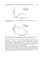
is a square wave with a frequency of 0.4 Hz. Fig
12 depicts the experimental position control results without and with integral action. The
upper part in Fig. 12 corresponds to the
x
i
coordinate whereas the bottom part corresponds
to the
y
i
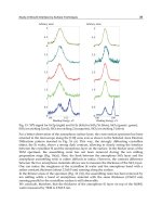
coordinate. Fig.13 depicts the image position errors; note that when the reference
changes, the position error settles around 0.5 pixels using the integral action. These results
indicate that the integral action removes the steady state error without greatly affecting the
transient response.


Fig. 11. Camera with image coordinate frame parallel to the robot coordinate frame.

Stable Visual PID Control of Redundant Planar Parallel Robots 47
Controls, model Junus 90 and working in current mode, drive the motors. Absolute optical encoders
from US Digital, model A2, with 4096 pulses per turn, supply measurements of the robot active and
passive joints angles
i
q
and
i
a
that allows computing the Jacobians

†
S and
( )
†
T
S .


Fig. 10. Laboratory prototype.

Two computers compose the control architecture; which is an update of the architecture
presented in (Soria et al. 2006). The first computer, called the vision computer and endowed
with an Intel Core2 processor running at 2.4 GHz, executes image acquisition; a Dalsa
Camera, model CA-1D-128A is connected to this computer by means of a National
Instruments card, model NI-1422. Image processing is performed using Visual C++ and the
DIAS software
1
. The second computer, called the control computer and endowed with an
Intel 4 processor running at 3.0 GHz, executes the control algorithm and performs data
logging. This computer receives data from the vision computer through an RS-232 port at
115 Kbaud. Data acquisition is carried out through a data card from Quanser consulting,
model MultiQ 3. This card reads signals from the optical incremental encoders attached to
the motors and supplies control voltages to the power amplifiers. Optical absolute encoders
connect to the control computer through an RS-232 using an AD2-B adapter from US
Digital.
Algorithms are coded using the Matlab/Simulink 5.2 software under the Wincon 3.02 real-
time environment. A counter in the MultiQ 3 card sets a sampling period of
0.5 ,
ie
T ms= which corresponds to the master clock of the closed-loop system; this sampling

period also sets the sampling time for reading the active joint incremental optical encoders.
The image sampling period is
5 ;
im
T ms= during this time interval, the vision computer
executes data acquisition and processing; it also includes the time required to send the robot
end-effector coordinates to the control computer through the RS-232 link. It is worth
mentioning that
im
T
corresponds to the time delay introduced in the visual measurements.
The absolute encoder measurements are sampled every
15
ab
T ms= . The sampling time for
the visual and absolute encoder, measurements are synchronized with the master clock. The
choice for the numerical method in Simulink was the ODE 45 Dormand-Price algorithm.
Gains for the proposed controller were set to
{
}
0.22 0.22 ,diag=
P
K
{
}
= 0.004 0.004diag
D
K ,
and
{

}
0.176 0.156diag=
I
K . The reference
*
x
i
is square wave of 16 pixels of amplitude, with
a frequency of 0.2 Hz, while the reference
*
y
i
is a square wave with a frequency of 0.4 Hz. Fig
12 depicts the experimental position control results without and with integral action. The
upper part in Fig. 12 corresponds to the
x
i
coordinate whereas the bottom part corresponds
to the
y
i
coordinate. Fig.13 depicts the image position errors; note that when the reference
changes, the position error settles around 0.5 pixels using the integral action. These results
indicate that the integral action removes the steady state error without greatly affecting the
transient response.



Fig. 11. Camera with image coordinate frame parallel to the robot coordinate frame.

PID Control, Implementation and Tuning48

Fig. 12. Desired and measured end effector positions: Left, without integral
action
{ }
= 0 0diag
I
K ; right, with integral action
{
}
0.176 0.156diag=
I
K .


Fig. 13. Image position errors: Left, without integral action; right, with integral action.

6. Conclusion
This chapter has presented some modeling and control issues related to a class of
overactuated planar parallel robots. After reviewing the kinematic and dynamic modeling
of this kind of robots, the Authors propose a novel imaged-based Proportional-Integral-
Derivative regulator. A key element in this control law is the measurement of the end-
effector position using a vision system. This feature avoids using the robot Forward
Kinematics employed traditionally for controlling planar parallel robots, and which requires
an off-line calibration. Moreover, the proposed control law does not rely on camera
calibration. A theoretical study provides conditions on the PID gains for obtaining
asymptotic closed-loop stability. A practical implementation of the proposed method using
a laboratory prototype shows a good performance of the closed-loop system. The
experiments indicate that, as expected in a PID controller, the integral action removes the
steady state error without a noticeable degradation in the transient response.

7. References
Angel, L.; Traslosheros, A.; Sebastian, J.M.; Pari, L.; Carelli, R. & Roberti, F. (2008). Vision-
based control of the robotenis system, Recent Progress in Robotics, Springer Verlag.
LNCIS 370, pp. 229-240.
Arimoto, S. & Miyazaki, F. (1984). Stability and robustness of PID feedback control for robot
manipulators of sensory capability, In: Robotics Research: First International
Symposium, Brady, M. & Paul, R. P., Ed. Cambridge, 783-799, MIT Press, MA.
Andreff, N. & Martinet, Ph. (2006). Unifying kinematic modeling, identification, and control
of a Gough-Stewart parallel robot into a vision-based framework, IEEE Trans. on
Robotics, Vol. 22, No. 6.
Andreff, N.; Dallej, T. & Martinet, Ph. (2007). Image-based Visual Servoing of a Gough-
Stewart Parallel Manipulator using Leg Observations, The International Journal of
Robotic Research, Vol. 26, pp. 667-687.
Chaumette, F. & Hutchinson, S. (2006). Visual servo control part I: Basic approaches. IEEE
Robotics & Automation Magazine, December 2006.
Chaumette, F. & Hutchinson, S. (2007). Visual servo control part II: Advanced approaches. IEEE
Robotics & Automation Magazine, March 2007.
Cheng, H.; Yiu, Y.K. & Li, Z. (2003). Dynamics and Control of Redundantly Actuated
Parallel Manipulators, IEEE/ ASME Transactions on Mechatronics, Vol. 8, No. 4,
December 2003, 483-491.
Corke, P. (1996). Visual Control of Robots: High performance Visual Servoing. Taunton,
Somerset, England: Research Studies Press.
Dallej, T.; Andreff, N. & Martinet, Ph. (2007). Image-based visual servoing of the I4R parallel
robot without propioceptive sensors. Proceedings of the Int. Conf. on Robotics and
Automation, Roma, Italy.
Hutchinson, S.; Hager, G.D. & Corke P.I. (1996) A tutorial on visual servo control. IEEE
Transactions on Robotics and Automation, Vol. 12, No. 5, October 1996, 651-670.
Kelly, R. (1995). A tuning procedure for stable PID control of robot manipulators, Robotica,
pt. 2, Vol. 13, Mar. /Apr. 1995, pp. 141-148.

Kelly, R. (1996). Robust Asymptotically Stable Visual Servoing of Planar Robots, IEEE
Transactions on Robotics and Automation, Vol. 12, No. 5, October 1996, 759-766.
Kelly, R. (1998). Global Positioning of Robot Manipulators via PD Control plus a Class of
Nonlinear Integral Actions, IEEE Transactions on Automatic Control, Vol. 43, No. 7,
July 1998, pp. 934-938.
Kock, S. & Schumacher, W. (1998). A Parallel x-y Manipulator with Actuation Redundancy
for High-Speed and Active-Stiffness Applications, Proceeding of the 1998 IEEE
International Conference on Robotics & Automation, pp. 2295-2300, Belgium, May 1998,
Leuven.
Kragic, D. & Christensen, H.I. (2005). Survey on Visual Servoing for Manipulation. Technical
report ISNR KTH/NA/P-02/01-SE, Department of Numerical Analysis and
Computing Science, University of Stockolm, Sweden.
Merlet, J.P. (2000). Parallel Robots, Klwuer Academic Publishers.
Papanikolopoulos, N. & Khosla, P. (1993). Adaptive Robotic Visual Tracking: Theory and
Experiments, IEEE Transactions on Automatic Control, Vol. 38, No. 3, March 1993,
429-444.
Stable Visual PID Control of Redundant Planar Parallel Robots 49

Fig. 12. Desired and measured end effector positions: Left, without integral
action
{
}
= 0 0diag
I
K ; right, with integral action
{
}
0.176 0.156diag=
I
K .

Fig. 13. Image position errors: Left, without integral action; right, with integral action.

6. Conclusion
This chapter has presented some modeling and control issues related to a class of
overactuated planar parallel robots. After reviewing the kinematic and dynamic modeling
of this kind of robots, the Authors propose a novel imaged-based Proportional-Integral-
Derivative regulator. A key element in this control law is the measurement of the end-
effector position using a vision system. This feature avoids using the robot Forward
Kinematics employed traditionally for controlling planar parallel robots, and which requires
an off-line calibration. Moreover, the proposed control law does not rely on camera
calibration. A theoretical study provides conditions on the PID gains for obtaining
asymptotic closed-loop stability. A practical implementation of the proposed method using
a laboratory prototype shows a good performance of the closed-loop system. The
experiments indicate that, as expected in a PID controller, the integral action removes the
steady state error without a noticeable degradation in the transient response.

7. References
Angel, L.; Traslosheros, A.; Sebastian, J.M.; Pari, L.; Carelli, R. & Roberti, F. (2008). Vision-
based control of the robotenis system, Recent Progress in Robotics, Springer Verlag.
LNCIS 370, pp. 229-240.
Arimoto, S. & Miyazaki, F. (1984). Stability and robustness of PID feedback control for robot
manipulators of sensory capability, In: Robotics Research: First International
Symposium, Brady, M. & Paul, R. P., Ed. Cambridge, 783-799, MIT Press, MA.
Andreff, N. & Martinet, Ph. (2006). Unifying kinematic modeling, identification, and control
of a Gough-Stewart parallel robot into a vision-based framework, IEEE Trans. on
Robotics, Vol. 22, No. 6.
Andreff, N.; Dallej, T. & Martinet, Ph. (2007). Image-based Visual Servoing of a Gough-
Stewart Parallel Manipulator using Leg Observations, The International Journal of

Robotic Research, Vol. 26, pp. 667-687.
Chaumette, F. & Hutchinson, S. (2006). Visual servo control part I: Basic approaches. IEEE
Robotics & Automation Magazine, December 2006.
Chaumette, F. & Hutchinson, S. (2007). Visual servo control part II: Advanced approaches. IEEE
Robotics & Automation Magazine, March 2007.
Cheng, H.; Yiu, Y.K. & Li, Z. (2003). Dynamics and Control of Redundantly Actuated
Parallel Manipulators, IEEE/ ASME Transactions on Mechatronics, Vol. 8, No. 4,
December 2003, 483-491.
Corke, P. (1996). Visual Control of Robots: High performance Visual Servoing. Taunton,
Somerset, England: Research Studies Press.
Dallej, T.; Andreff, N. & Martinet, Ph. (2007). Image-based visual servoing of the I4R parallel
robot without propioceptive sensors. Proceedings of the Int. Conf. on Robotics and
Automation, Roma, Italy.
Hutchinson, S.; Hager, G.D. & Corke P.I. (1996) A tutorial on visual servo control. IEEE
Transactions on Robotics and Automation, Vol. 12, No. 5, October 1996, 651-670.
Kelly, R. (1995). A tuning procedure for stable PID control of robot manipulators, Robotica,
pt. 2, Vol. 13, Mar. /Apr. 1995, pp. 141-148.
Kelly, R. (1996). Robust Asymptotically Stable Visual Servoing of Planar Robots, IEEE
Transactions on Robotics and Automation, Vol. 12, No. 5, October 1996, 759-766.
Kelly, R. (1998). Global Positioning of Robot Manipulators via PD Control plus a Class of
Nonlinear Integral Actions, IEEE Transactions on Automatic Control, Vol. 43, No. 7,
July 1998, pp. 934-938.
Kock, S. & Schumacher, W. (1998). A Parallel x-y Manipulator with Actuation Redundancy
for High-Speed and Active-Stiffness Applications, Proceeding of the 1998 IEEE
International Conference on Robotics & Automation, pp. 2295-2300, Belgium, May 1998,
Leuven.
Kragic, D. & Christensen, H.I. (2005). Survey on Visual Servoing for Manipulation. Technical
report ISNR KTH/NA/P-02/01-SE, Department of Numerical Analysis and
Computing Science, University of Stockolm, Sweden.
Merlet, J.P. (2000). Parallel Robots, Klwuer Academic Publishers.

Papanikolopoulos, N. & Khosla, P. (1993). Adaptive Robotic Visual Tracking: Theory and
Experiments, IEEE Transactions on Automatic Control, Vol. 38, No. 3, March 1993,
429-444.
PID Control, Implementation and Tuning50
Santibañez, V. & Kelly, R. (1998). A Class of Nonlinear PID Global Regulators for Robot
Manipulators”, Proc. IEEE Int. Conf. on Robotics and Automation, pp. 3601-3606.
Sebastian, J.M.; Traslosheros, A.; Angel, L.; Roberti, F. & Carelli, R. (2007). Parallel robot high
speed object tracking. M. Kamel and A. Campilho (Eds.): ICIAR 2007, LNCS 4633, pp.
295.306.
Soria, A.; Garrido, R.; Vásquez, I. & Vázquez ,R. (2006). Architecture for rapid prototyping of visual
controllers. Robotics and Autonomous Systems, Vol. 54, pp. 486-495.
Spong, M.W.; Hutchinson, S. & Vidyasagar, M. M.W. (2005) Robot Modeling and Control,
Wiley.
Tsai, L.W. (1999). Robot Analysis. John Wiley and Sons Inc.
Weiss, L.; Sanderson, A. & Newman, C. (1987). Dynamic Sensor-Based Control of Robots
with Visual Feedback, IEEE Journal of Robotics and Automation, Vol. RA-3, No. 5,
October 1987, 404-417.
Wen, J. T. & Murphy, S. (1990). PID control for robot manipulators, CIRSSE Document # 54,
Rensselaer Polytechnic Institute.
Wilson, W.; Williams Hulls, C. & Bell, G. (1996). Relative End-Effector Control Using
Cartesian Position Based Visual Servoing, IEEE Transactions on Robotics and
Automation, Vol. 12, No.5, October 1996, pp. 684-696.



1
Voss, K.; Ortmann,W. & Suesse, H. (1998). DIAS-Interactive Image Processing System, V 5.0,
Friedrich-Schiller-University Jena, Germany.

Pid Controller with Roll Moment Rejection for Pneumatically Actuated

Active Roll Control (Arc) Suspension System
Khisbullah Hudha, Fauzi Ahmad, Zulkifi Abd. Kadir and Hishamuddin Jamaluddin
X

Pid Controller with Roll Moment Rejection
for Pneumatically Actuated Active Roll
Control (Arc) Suspension System

Khisbullah Hudha
1)
, Fauzi Ahmad
1)
, Zulkiffli Abd. Kadir
2)

and Hishamuddin Jamaluddin
3)
1)
Vehicle Control and Biomechanics Research Group
for Vehicle Research and Development (CeVReD)

Universiti Teknikal Malaysia Melaka (UTeM)
Hang Tuah Jaya, 76100 Durian Tunggal Melaka.
2)
Dept. of Mech. Eng., Faculty of Engineering
Universiti Pertahanan Nasional Malaysia (UPNM)
Kem Sungai Besi, 57000 Kuala Lumpur, Malaysia
3)
Faculty of Mechanical Engineering
Universiti Teknologi Malaysia (UTM)

81310 UTM Skudai, Johor, Malaysia

Abstract
This chapter presents a successful implementation of PID controller for a pneumatically
actuated active roll control suspension system in both simulation and experimental studies.
For the simulation model, a full vehicle model which consists of ride, handling and tire
subsystems to study vehicle dynamics behavior in lateral direction is derived. The full
vehicle model is then validated experimentally using an instrumented experimental vehicle
based on the driver input from the steering wheel. Two types of vehicle dynamics test are
performed for the purpose of model validation namely step steer test and double lane
change test. The results of model validation show that the behaviors of the model closely
follow the behavior of a real vehicle with acceptable error. An active roll control (ARC)
suspension system is then developed on the validated full vehicle model to reduce
unwanted vehicle motions during cornering maneuvers such as body roll angle, body roll
rate, vertical acceleration of the body and body heave. The proposed controller structure for
the ARC system is PID control with roll moment rejection loop. The ARC system is then
implemented on an instrumented experimental vehicle in which four units of pneumatic
actuators are installed in parallel arrangement with the passive suspension system. The
results of the study shows that the proposed control structure is able to significantly
improve the dynamics performance of the vehicle during step steer and double lane change
maneuvers compared to a passive vehicle system. It can also be noted that the additional
3
PID Control, Implementation and Tuning52
roll moment rejection loop is able to further improve the performance of the PID controller
for the ARC system.

1. Introduction
PID controller is the most popular feedback controller used in the process industries. The
algorithm is simple but it can provide excellent control performance despite variation in the
dynamic characteristics of a process plant. PID controller is a controller that includes three

elements namely proportional, integral and derivative actions. The PID controller was first
placed on the market in 1939 and has remained the most widely used controller in process
control until today (Araki, 2006). A survey performed in 1989 in Japan indicated that more
than 90% of the controllers used in process industries are PID controllers and advanced
versions of the PID controller (Takatsu et al., 1998).

The use of electronic control systems in modern vehicles has increased rapidly and in recent
years, electronic ontrol systems can be easily found inside vehicles, where they are
responsible for smooth ride, cruise control, traction control, anti-lock braking, fuel delivery
and ignition timing. The successful implementation of PID controller for automotive
systems have been widely reported in the literatures such as for engine control (Ying et al.,
1999; Yuanyuan et al., 2008; Bustamante et al., 2000), vehicle air conditioning control (Zhang
et al., 2010), clutch control (Wu et al., 2008; Wang et al., 2001 ), brake control (Sugisaka et al.,
2006; Hashemi-Dehkordi et al., 2009; Zhang et al., 1999), active steering control (Marino et al.,
2009; Yan et al., 2008), power steering control (Morita et al., 2008), drive train control
(Mingzhu et al., 2008; Wei et al., 2010; Xu, et al., 2007), throttle control (Shoubo et al., 2009;
Tan et al., 1999; Corno et al., 2008) and suspension control ( Ahmad et al., 2008; Ahmad et al.,
2009a; Ahmad et al., 2009b; Hanafi, 2010; Ayat et al., 2002a ).

Over the last two decades, various active chassis control systems for automotive vehicles
have been developed and put to commercial utilization. In particular, Vehicle Dynamics
Control (VDC) and Electronic Stability Program (ESP) systems have become very active and
attracting research efforts from both academic community and automotive industries
(Mammar and Koenig, 2002; McCann, 2000; Mokhiamar and Abe, 2002; Wang and Longoria,
2006). The main goals of active chassis control include improvement in vehicle stability,
maneuverability and passenger comfort especially in adverse driving conditions.

Ignited by advanced electronic technology, many different active chassis control systems
have been developed, such as traction control system (Borrelli et al., 2006), active steering
control (Falcone et al., 2007), antilock braking system (Cabrera et al., 2005), active roll control

suspension system and others. This study is part of the continuous efforts in the prototype
development of a pneumatically actuated active roll control suspension system for
passenger vehicles. The proposed ARC system is used to minimize the effects of unwanted
roll and vertical body motions of the vehicle in the presence of steering wheel input from the
driver.

ARC system is a class of electronically controlled active suspension system. Although active
suspension has been widely studied for decades, most of the research are focused on vehicle
ride comfort, with only few papers (Williams and Haddad, 1995; Ayat et al., 2002a; Wang et
al., 2005, Ayat et al., 2002b) studying how an active suspension system can improve vehicle
handling. It is well-known that a vehicle tends to roll on its longitudinal axis if the vehicle is
subjected to steering wheel input due to the weight transfer from the inside to the outside
wheels. Some control strategies for ARC systems have been proposed to cancel out lateral
weight transfer using active force control strategy (Hudha et al. 2003), hybrid fuzzy-PID
(Xinpeng and Duan, 2007), speed dependent gain scheduling control (Darling and Ross-
Martin, 1997), roll angle and roll moment control (Miege and Cebon, 2002), state feedback
controller optimized with genetic algorithm (Du and Dong, 2007) and the combination of
yaw rate and side slip angle feedback control (Sorniotti and D’Alfio, 2007).

In this study, ARC system is developed using four units of pneumatic system installed
between lower arms and vehicle body. The proposed control strategy for the ARC system is
the combination of PID based feedback control and roll moment rejection based feed
forward control. Feedback control is used to minimize unwanted body heave and body roll
motions, while the feed forward control is intended to reduce the unwanted weight transfer
during steering input maneuvers. The forces produced by the proposed control structure are
used as the target forces by the four unit of pneumatic system.

The use of pneumatic actuator for an active roll control suspension system is a relatively
new concept and has not been thoroughly explored. The use of pneumatic system is rare in
active suspension application although they have several advantages compared with other

actuation systems such as hydraulic system. The main advantage of pneumatic system is
their power-to-weight ratio which is better than hydraulic system. They are also clean,
simple system and comparatively low cost (Smaoui et al., 2006). The disadvantage of
pneumatic system is the unwanted nonlinearity because of the compressibility and
springing effects of air (Situm et al., 2005; Richer and Hurmuzlu, 2000). Due to these
difficulties, early use of pneumatic actuators was limited to simple applications that
required only positioning at the two ends of the stroke. But, during the past decade, many
researchers have proposed various approaches to continuously control the pneumatic
actuators (Ben-Dov and Salcudean, 1995; Wang et al., 1999; Messina et al., 2005). It is shown
that the comparative advantages and difficulties of pneumatic system are still interesting
and also a challenging problems in controller design in order to achieve reasonable
performance in terms of position and force controls.

The proposed control strategy is optimized for a 14 degrees of freedom (DOF) full vehicle
model. The full vehicle model consists of 7-DOF vehicle ride model and 7-DOF vehicle
handling model coupled with Calspan tyre model. The full vehicle model can be used to
study the behavior of vehicle in lateral, longitudinal and vertical directions due to both road
and driver inputs. Calspan tire model is employed due to its capability to predict the
behavior of a real tire better than Dugoff and Magic formula tire model (Kadir et al., 2008).

Beside the proposed control structure, another consideration of this chapter is that the
proposed control structure for the ARC system is implemented on a validated full vehicle
model as well as on a real vehicle. It is common that the controllers, developed on the
validated model, are ready to be implemented in practice with high level of confidence and