Robust Control Theory and Applications Part 15 docx

Robust Bilateral Control for Teleoperation System with Communication Time Delay
- Application to DSD Robotic Forceps for Minimally Invasive Surgery -

547
one joint is between -30 and +30 degrees since this is the allowable bending angle of the
universal joint. One bending linkage allows for one-DOF bending motion, and by using two
bending linkages and controlling their rotation angles, arbitrary omnidirectional bending
motion can be attained. The total length of the bending part is 59 mm excluding a gripper.
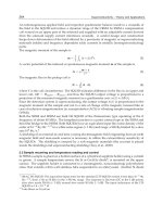
2.3 Attachment and rotary gripper
The gripper is exchangeable as an end effector and can be replaced with tools such as
scalpels or surgical knives. Fig. 5 shows the attachment of the end effecter and mechanism of
the rotary gripper. Gear 1 is on the tip of the grasping linkage and gear 2 is at the root of the
jaw mesh. The gripper is turned by rotation of the grasping linkage. Although the rotary
gripper can rotate arbitrary degrees, it should be rotated within 360 degrees to avoid
winding of the wire which drives the jaw.

Gear1
Gear2
End effecter
End plate
Gear1
Gear2
Gear1
Gear2
End effecter
End plate
End effecter
End plate

Fig. 5. Attachment and rotation of gripper
2.4 Open and close of jaws

The opening and closing motions of the gripper are achieved by wire actuation. Only one
side of the jaws can move, and the other side is fixed. The wire for actuation connects to the
drive unit through the inside of the DSD mechanism and the rod, and is pulled by the
motor. The open and closed states of the gripper are shown in Fig.6.

Open Close
Wire
Open Close
Wire

Fig. 6. Grasping of gripper
2.5 Drive unit
The feature of a drive unit for the DSD robotic forceps manipulator is shown in Fig.7. The
total length of the drive unit is 274 mm, its maximum diameter is 50 mm, and its weight is
935 g. Driving forces from motors are transmitted to the linkages through the gears. There
Robust Control, Theory and Applications

548
are four motors in the drive unit. Three motors are mounted at the center of the drive unit.
Two of them are used for inducing bending motion and the third one is used for inducing
rotary motion of the gripper. The fourth motor, which is mounted in the tail, is for the
opening and closing motions of the gripper actuated by wire. The wire capstan is attached to
the motor shaft of the forth motor and acts as a reel for the wire. The spring is used for
maintaining the tension of the wire. DC micromotors 1727U024C (2.25W) produced by
FAULHABER Co. were selected for the bending motion and the rotary motion of the
gripper. For the opening and closing motions of the gripper, a DC micro motor 1727U012C
(2.25W) produced by FAULHABER Corp. was selected. A reduction gear and a rotary
encoder are installed in the motor.

Wire CapstanWire

274
50
Spring
Gear C
Gear A Gear B
Wire CapstanWire
274
50
Spring
Gear C
Gear A Gear B

Fig. 7. Drive unit
The inside part of the rod, as shown in Fig. 1, consists of three shafts, each 2 mm in diameter
and 300 mm long. Each motor in the drive unit and each linkage in the DSD mechanism are
connected to each other through a shaft. Therefore, the rotation of each motor is transmitted
to each respective linkage through a shaft.
2.6 Built DSD robotic forceps manipulator
The proposed DSD robotic forceps manipulator was built from stainless steel SUS303 and
SUS304 to satisfy bio-compatibility requirements. The miniature universal joints produced
by Miyoshi Co., LTD. were selected. The universal joints have a diameter of 3 mm and are of
the MDDS type. The screws on both sides of the yokes were fabricated by special order.
The built DSD robotic forceps manipulator is shown in Fig. 8. Its maximum diameter from
the top of the bending part to the root of the rod is 10 mm. The total length of the bending
part, including the gripper, is 85 mm.


Fig. 8. Built DSD robotic forceps manipulator
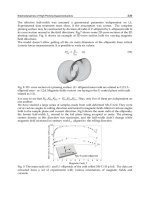
A transition chart of the rotary gripper is shown in Fig.9.
Robust Bilateral Control for Teleoperation System with Communication Time Delay

- Application to DSD Robotic Forceps for Minimally Invasive Surgery -

549

Fig. 9. Transition chart of the rotary gripper
2.7 Master manipulator for teleoperation
In a laparoscopic surgery, multi-DOF robotic forceps manipulators are operated by remote
control. In order to control the DSD robotic forceps as a teleoperation system, the joy-stick
type master manipulator for teleoperation was designed and built in (Ishii et al., 2010) by
reconstruction of a ready-made joy-stick combined with the conventional forceps, which
enables to control bending, grasping and rotary motions of the DSD robotic forceps
manipulator. In addition, the built joy-stick type master manipulator was modified so that
the operator can feel reaction force generated by the electric motors. The teleoperation
system and the force feedback mechanisms for the bending force are illustrated in Fig.10.
The operation force is detected by the strain gauges, and variation of the position is
measured by the encoders mounted in the electric motors.

Strain gauge
Bending
Strain gauge
Motor with
rotary encoder
Joystick
Master Slave
m
x
s
x
s
f

m
f
Strain gauge
Bending
Strain gauge
Motor with
rotary encoder
Joystick
Strain gauge
Bending
Strain gauge
Motor with
rotary encoder
Joystick
Master Slave
m
x
s
x
s
f
m
f

Fig. 10. DSD robotic forceps teleoperation system
3. Bilateral control for one-DOF bending
In this section, bilateral control law for one-DOF bending of the DSD robotic forceps
teleoperation system with communication time delay is derived.
3.1 Derivation of Control Law
Let the dynamics of the one-DOF master-slave teleoperation system be given by

mm mm mm m m
mx bx cx f++=τ+
 
, (1)
Robust Control, Theory and Applications

550

ss ss ss s s
mx bx cx f
+
+=τ−
 
, (2)
where subscripts m and s denote master and slave respectively. x
m
and x
s
represent the
displacements, m
m
and m
s
the masses, b
m
and b
s
the viscous coefficients, and c
m

and c
s
the
spring coefficients of the master and slave devices. f
m
stands for the force applied to the
master device by human operator, f
s
the force of the slave device due to the mechanical
interaction between slave device and handling object, and
m
τ
and
s
τ
are input motor
toques.
As shown in Fig.11, there exists constant time delay T in the network between the master
and the slave systems.

Human
operator
Master Slave Environment
m
x
s
x
m
f
s

f
T
T
Communication Time Delay
Human
operator
Master Slave Environment
m
x
s
x
m
f
s
f
T
T
Communication Time Delay

Fig. 11. Communication time delay in teleoperation systems
Define motor torques as

mmmmmmmm
xcxbxm
+
−
−
=
λ
λ

τ
τ

, (3)

ssssssss
xcxbxm
+
−
−
=
λ
λ
τ
τ

, (4)
where λ is a positive constant, and
m
τ
and
s
τ are coupling torques. Then, the dynamics
are rewritten as follows.

mmmmmm
frbrm
+
=
+

τ

, (5)

ssssss
frbrm
−
=
+
τ

, (6)
where r
m
and r
s
are new variables defined as

mmm
xxr
λ
+=

, (7)

sss
xxr
λ
+
=


. (8)
Control objective is described as follows.
[Design Problem] Find a bilateral control law which satisfies the following two
specifications.
Specification 1: In both position tracking and force tracking, the motion scaling, which can
adequately reduce or enlarge the movements and tactile senses of the master device and the
slave device, is achievable.
Specification 2: The stability of the teleoperation system in the presence of the constant
communication time delay between master device and slave device, is guaranteed.
Robust Bilateral Control for Teleoperation System with Communication Time Delay
- Application to DSD Robotic Forceps for Minimally Invasive Surgery -

551
Assume the following condition.
Assumption: The human operator and the remote environment are passive.
In the presence of the communication time delay between master device and slave device,
the following fact is shown in (Chopra et al., 2003).
Fact: In the case where the communication time delay
T is constant, the teleoperation
system is passive.
From Assumption and Fact, the following inequalities hold.

00
0, 0
tt
mm ss
rfd rfd
−
τ≥ τ≥

∫∫
, (9)

() ()
00
0, 0
tt
sm ms
rf Td rf Td
−
τ− τ≥ τ− τ≥
∫∫
. (10)
Using inequalities (9) and (10), define a positive definite function V as follows.

()
()
()
() ()
22 222
1
00
00
21 2 1
22
t
mm p ss m p s
tT
tt
mmmpfsss

tt
ps sm f m ms
Vmr Gmr K r Grd
KrfdGGKrfd
GK rf Td GK rf Td
−
=+ + + τ
−
+τ+ +τ
−
τ− τ+ τ− τ
∫
∫∫
∫∫
, (11)
where
1
K
,
m
K
and
s
K
are feedback gains, and 1
p
G ≥ and 1
f
G ≥ are scaling gains for
position tracking and force tracking, respectively.

The derivative of V along the trajectories of the systems (5) and (6) is given by

(
)
() ()
()
()
()
() ()
()()
()
()
()
()
()
()
()
()
()
222
1
222
1
1
1
22

21 2 1
22
22

21
mmm p sss m p s
mps
mmmpfsss
pssm f mms
mmmmm
p
sssss
ps m ps m
mpsmps
m
Vmrr GmrrKr Gr
Kr tT Gr tT
KrfGGKrf
GKrf tT GKrftT
rbr f Grbr f
KGrtT r GrtT r
KrtT Gr rtT Gr
K
=+ ++
−−+−
−+ + +
−−+ −
=−+τ++ −+τ−
−−− −+
−−− −+
−+



()
() ()
21
22.
mm p f s ss
pssm f mms
rf G GK rf
GKrf tT GKrftT
++
−−+ −
(12)
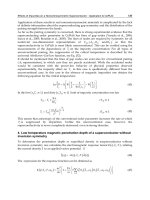
Let the coupling torques be given as follows.

()
(
)
()
(
)
1m
p
smm
f
sm
KGrtT r K G
f
tT
f
τ= − − − − − , (13)

()
(
)
()
(
)
1sm
p
ssm
f
s
KrtT Gr K
f
tT G
f
τ= − − + − − . (14)
Robust Control, Theory and Applications

552
Using (13) and (14), (12) is rewritten as follows.

()
()
{}
()
()
{}
()
()

{}
()
()
{}
()
()
() ()
22
1
1
1
1
2
2222 2 2
2
2
21 2 1
22
2
mm m m m m p ss ps s ps s
mmfs m m mmfs m
ssm fs ps ssm fs
mmmpfss
pssm f mms
mm
Vbr r rfGbrGr Grf
K GftT f r K K GftT f
KftT Gf Gr K KftT Gf
KrfGGKrf
GKrf t T GK r f t T

br
−
−
=− + τ + − + τ −
⎡
⎤
+τ+ − − + τ+ − −
⎢
⎥
⎣
⎦
⎡
⎤
−τ− − − + τ− − −
⎢
⎥
⎣
⎦
−+ + +
−−+ −
=−

()
()
{}
()
()
{}
()
()

()
()
2
22
11
11
22
11
2

.
pss
m m fs m s s m fs
ps m m ps
Gbr
K K GftT f K Kf tT Gf
KGrtT r KrtT Gr
−−
−
−τ+ −− −τ− −−
≤− − − − − −
(15)
Thus, stability of the teleoperation system is assured in spite of the presence of the constant
communication time delay, and delay independent exponential convergence of the tracking
errors of position to the origin is guaranteed.
Finally, motor torques (3) and (4) are given as follows.

()
()
11

11
() () ()
()
mps ps mfs
mm m m m mm
KGx t T KGx t T K G f t T
Kmxc KbxKf
τ
=−+λ−− −
−+λ +−λ+ +


, (16)

()( )
11
11
() () ()
()
sm m sm
p
ss s
p
ss ss
Kx t T Kx t T Kf t T
KG m x c KG b x K
f
τ
=−+λ−+−
−+λ+−λ+−



. (17)
3.2 Experiments
In order to verify an effectiveness of the proposed control law, experimental works were
carried out for the developed DSD robotic forceps teleoperation system. Here, only vertical
direction of the bending motion is considered. Namely, bending motion of the DSD robotic
forceps is restricted to one degree of freedom. Then, the dynamics of the master-slave
teleoperation system are given by equations (1) and (2), since only one bending linkage is
used. Parameter values of the system are given as
m
m
= 0.07 kg, m
s
= 0.025 kg, b
m
= 0.25
Nm/s,
b
s
= 2.5 Nm/s, c
m
= 9 N/s and c
s
= 9 N/s. The control system is constructed under the
MATLAB/Simulink software environment.
In the experiments, 200g weights pet bottle filled with water was hung up on the tip of the
forceps, and lift and down were repeated in vertical direction. Appearance of the
experiment is shown in Fig. 12.
First, in order to see the effect of the motion scaling, experimental works with the following

conditions were carried out.
a.
Verification of the effect of the motion scaling.
i)
G
p
= G
f
= 1 and T = 0
ii)
G
p
= 2, G
f
= 3 and T = 0
Second, in order to see the effect to the time delay, comparison of the proposed bilateral
control scheme and conventional bilateral control method was performed.
Robust Bilateral Control for Teleoperation System with Communication Time Delay
- Application to DSD Robotic Forceps for Minimally Invasive Surgery -

553

Fig. 12. Appearance of experiment
b.
Verification of the effect to the time delay.
i)
G
p
= G
f

= 1 and T = 0.125
ii) Force reflecting servo type bilateral control law with constant time delay
T = 0.125
In b-ii), the force reflecting servo type bilateral control law is given as follows.

(
)
()
mfms
Kf ftTτ= − − , (18)

(
)
()
s
p
ms
KxtT xτ= − −
, (19)
where
K
f
and K
p
are feedback gains of force and position. The time delay T = 0.125 is
intentionally generated in the control system, whose value was referred from (Arata et al.,
2007) as the time delay of the control signal between Japan and Thailand: approximately
124.7 ms.

0 5 10 15 20 25 30 35

-4
-2
0
2
4
Force
Time [s]
f
s
and f
m
[N]


0 5 10 15 20 25 30 35
-30
-20
-10
0
10
20
30
Position
Time [s]
x
s
and x
m
[mm]

xs
xm
fs
fm

Fig. 13. Experimental result for a-i)
Robust Control, Theory and Applications

554
0 5 10 15 20 25 30 35 40 45
-4
-2
0
2
4
6
8
Force
Time [s]
f
s
and f
m
[N]


0 5 10 15 20 25 30 35 40 45
-30
-20

-10
0
10
20
30
Position
Time [s]
x
s
and x
m
[mm]


xs
xm
fs
fm

Fig. 14. Experimental result for a-ii)
Note that the proposed bilateral control scheme guarantees stability of the teleoperation
system in the presence of constant time delay, however, stability is not guaranteed in use of
the force reflecting servo type bilateral control law in the presence of constant time delay.
Feedback gains were adjusted by trial and error through repetition of experiments, which
were determined as
λ
= 3.8, K
1
= 30, K
m

= 400, K
s
= 400, K
p
= 60 and K
f
= 650. Experimental
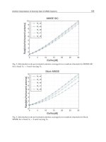
results for condition a) are shown in Fig. 13 and Fig. 14.
As shown in Fig. 13 and Fig. 14, it is verified that the motion of slave tracks the motion of
master with specified scale in both position tracking and force tracking.
Experimental results for condition b) are shown in Fig. 15 and Fig. 16.

0 5 10 15 20 25 30
-4
-2
0
2
4
Force
Time [s]
f
s
and f
m
[N]


0 5 10 15 20 25 30
-30
-20

-10
0
10
20
30
Position
Time [s]
x
s
and x
m
[mm]


xs
xm
fs
fm

Fig. 15. Experimental result for b-i)
Robust Bilateral Control for Teleoperation System with Communication Time Delay
- Application to DSD Robotic Forceps for Minimally Invasive Surgery -

555
0 5 10 15 20 25 30 35
-4
-2
0
2
4

Force
Time [s]
f
s
and f
m
[N]


0 5 10 15 20 25 30 35
-30
-20
-10
0
10
20
30
Position
Time [s]
x
s
and x
m
[mm]


xs
xm
fs
fm

Fig. 16. Experimental result for b-ii)
As shown in Fig. 15 and Fig. 16, tracking errors of both position and force in Fig. 15 are
smaller than those of Fig. 16. From the above observations, the effectiveness of the proposed
control law for one-DOF bending motion of the DSD robotic forceps was verified.
4. Bilateral control for omnidirectional bending
In this section, the bilateral control scheme described in the former session is extended to
omnidirectional bending of the DSD robotic forceps teleoperation system with constant time
delay.
4.1 Extension to omnidirectional bending
As shown in Fig.10, master device is modified joy-stick type manipulator. Namely, this is
different structured master-slave system. The cross-section views of shaft of the joy-stick
and the DSD robotic forceps are shown in Fig.17.
Due to the placement of strain gauges and motors with encoder of the master device, the
dynamics of the master device are given in
x-y coordinates as follows.

mm mm mm xm xm
mx bx cx f
+
+=τ+
 
, (20)

mm mm mm ym ym
m
y
b
y
c

yf
+
+=τ+
 
. (21)
When only motor
A drives, bending direction of the DSD robotic forceps is along A-axis,
and when only motor
B drives, bending direction of the DSD robotic forceps is along B-axis.
Thus, due to the arrangement of the bending linkages, the dynamics of the slave device are
given in
A-B coordinates as follows.

ss ss ss As As
mA bA cA
f
++=τ−
 
, (22)

ss ss ss Bs Bs
mB bB cB
f
++=τ−
 
. (23)
Robust Control, Theory and Applications

556
B

A
),(
mm
yxr
),(
ss
yxr
Slave device
ym
τ
xm
τ
Master device
:Strain gauge
Bs
τ
As
τ
y
x
Motor1
Motor2
Motor A Motor B
：Shaft of joystick
：Cross-section of DSD forceps
：Bending linkage
y
x
s
A

s
B
m
x
m
y
：Grasping linkage
B
A
),(
mm
yxr
),(
ss
yxr
Slave device
ym
τ
xm
τ
Master device
:Strain gauge:Strain gauge
Bs
τ
As
τ
y
x
Motor1
Motor2

Motor A Motor B
：Shaft of joystick：Shaft of joystick
：Cross-section of DSD forceps：Cross-section of DSD forceps
：Bending linkage
：Bending linkage
y
x
s
A
s
B
m
x
m
y
：Grasping linkage：Grasping linkage

Fig. 17. Coordinates of master device and slave device
In order to extend the proposed bilateral control law to the omnidirectional bending motion
of the DSD robotic forceps, the coordinates must be unified.
As shown in Fig. 17,
x
m
and y
m
are measured by encoders. f
xm
, f
ym
, f

xs
, and f
ys
are measured by
strain gauges.
xm
τ
,
y
m
τ
,
xs
τ
and
y
s
τ
are calculated from the bilateral control laws. These
values are obtained in
x-y coordinates. Therefore, consider to unify the coordinates in x-y
coordinates. While, displacement of the slave
A
s
and B
s
are measured by encoder, which are
obtained in
A-B coordinates. These values must be changed into x-y coordinates.

y
x
B
A
),( yxr
),( BAr
θ
°30
°60
°90
x-y coordinate
A-B coordinate
: Angle of Rotation: Angle of Bend
θ
φ
φ
°120
y
x
B
A
),( yxr
),( BAr
θ
°30
°60
°90
x-y coordinate
A-B coordinate
: Angle of Rotation: Angle of Bend

θ
φ
φ
°120

Fig. 18. Change of coordinates
The change of coordinates for position
r(A,B) given in A-B coordinates to r(x,y) given in x-y
coordinates (Fig. 18) is given as follows.
Robust Bilateral Control for Teleoperation System with Communication Time Delay
- Application to DSD Robotic Forceps for Minimally Invasive Surgery -

557

33
1
2
11
xA
y
B
⎡⎤
⎡
⎤⎡⎤
−
=
⎢⎥
⎢
⎥⎢⎥
⎢⎥

⎣
⎦⎣⎦
⎣⎦
. (24)
Thus, the dynamics of the slave device given in A-B coordinates are converted into x-y
coordinates. Finally, the dynamics of the two-DOF DSD robotic forceps teleoperation system
in horizontal direction and vertical direction are described as follows.

mm mm mm xm xm
ss ss ss xs xs
mx bx cx f
mx bx cx f
++=τ+
⎧
⎨
++=τ−
⎩
 
 
(25)

mm mm mm
y
m
y
m
ss ss ss ys ys
my by cy f
my by cy f
++=τ+

⎧
⎪
⎨
++=τ−
⎪
⎩
 
 
(26)
For each direction, the bilateral control law derived in the former session, which is
developed for one-DOF bending of the DSD robotic forceps, is applied.
However, as shown in Fig. 17, the actual torque inputs to the motors in the slave device are
A
s
τ and
Bs
τ . Therefore, input torque of the slave must be given in A-B coordinates.
A
s
τ and
Bs
τ can be obtained from
xs
τ
and
y
s
τ
through an inverse transformation of (24), which is
given by

1/ 3 1
1/ 3 1
xs
As
y
s
Bs
⎡⎤
τ
⎡
⎤
τ
⎡⎤
=
⎢⎥
⎢
⎥
⎢⎥
τ
τ
−
⎢⎥
⎣⎦
⎣
⎦
⎣⎦
. (27)
Thus, bilateral control for the omnidirectional bending motion of the DSD robotic forceps is
realized.

4.2 Experiments
Experimental works were carried out using the proposed bilateral control laws. The
parameter values of the system are given as same value as described in subsection 3.2.
In the experiments, 100g weight pet bottle filled with water was hung up on the tip of the
forceps, and the pet bottle was lifted by vertical bending motion of the forceps. Then, the
forceps was controlled so that the tip of the forceps draws a quarter circular orbit
counterclockwise, and the PET bottle was landed on the floor.
Experimental works were carried out under the communication time delay T = 0.125. The
control gains were determined by trial and error through the repetition of experiments,
which are given as
λ
= 5.0, K
1
= 40, K
m
= 80, and K
s
= 80. Scaling gains were chosen as G
p
=
G
f
= 1. Experimental results are shown in Fig. 19.
In Fig. 19, the top two figures show force and position in x coordinates, and the bottom two
figures show force and position in y coordinates. In the experiment, the PET bottle was lifted
at around 4 seconds, and landed on the floor at around 20 seconds. The counterclockwise
rotation at the tip of the forceps has begun from around 12 seconds.
Although small tracking errors can be seen, the reaction forces which acted on the slave
device in x-y directions were reproducible to the master manipulator as tactile sense. In
terms of above observations, it can be said that the effectiveness of the proposed control

scheme was verified.
Robust Control, Theory and Applications

558
0 5 10 15 20 25 30
-40
-20
0
20
40
Position
Time [s]
x
s
and x
m
[m]


0 5 10 15 20 25 30
-1
-0.5
0
0.5
1
Force
Time [s]
f
xs
and f

xm
[N]


fxs
fxm
xs
xm

0 5 10 15 20 25 30
-40
-20
0
20
40
Position
Time [s]
y
s
and y
m
[m]


0 5 10 15 20 25 30
-1
-0.5
0
0.5
1

Force
Time [s]
f
ys
and f
ym
[N]


fys
fym
ys
ym

Fig. 19. Experimental results for omnidirectional bending of DSD robotic forceps
5. Conclusion
In this chapter, robust bilateral control for teleoperation systems in the presence of
communication time delay was discussed. The Lyapunov function based bilateral control
law that enables the motion scaling in both position tracking and force tracking, and
guarantees stability of the system in the presence of the constant communication time delay,
was proposed under the passivity assumption.
The proposed control law was applied to the haptic control of one-DOF bending motion of
the DSD robotic forceps teleoperation system with constant time delay, and experimental
works were executed.
Robust Bilateral Control for Teleoperation System with Communication Time Delay
- Application to DSD Robotic Forceps for Minimally Invasive Surgery -

559
In addition, the proposed bilateral control scheme was extended so that it may become
applicable to the omnidirectional bending motion of the DSD robotic forceps. Experimental

works for the haptic control of omnidirectional bending motion of the DSD robotic forceps
teleoperation system with constant time delay were carried out. From the experimental
results, the effectiveness of the proposed control scheme was verified.
6. Acknowledgement
The part of this work was supported by Grant-in-Aid for Scientific Research(C) (20500183).
The author thanks H. Mikami for his assistance in experimental works.
7. References
Anderson, R. & Spong, M. W. (1989). Bilateral Control of Teleoperators with Time Delay,
IEEE Transactions on Automatic Control, Vol.34, No. 5, pp.494-501
Arata, J., Mitsuishi, M., Warisawa, S. & Hashizume, M. (2005). Development of a Dexterous
Minimally-Invasive Surgical System with Augumented Force Feedback Capability,
Proceedings of 2005 IEEE/RSJ International Conference on Intelligent Robots and Systems,
pp.3207-3212
Arata, J., Takahashi, H., Pitakwatchara, P., Warisawa, S., Tanoue, K., Konishi, K., Ieiri, S.,
Shimizu, S., Nakashima, N., Okamura, K., Fujino, Y., Ueda, Y., Chotiwan, P.,
Mitsuishi, M. & Hashizume, M. (2007). A Remote Surgery Experiment Between
Japan and Thailand Over Internet Using a Low Latency CODEC System,
Proceedings of IEEE International Conference on Robotics and Automation, pp.953-959
Chopra, N., Spong, M. W., Hirche, S. & Buss, M. (2003). Bilateral Teleoperation over the
Internet: the Time Varying Delay Problem, Proceedings of the American Control
Conference, pp.155-160
Chopra, N. & Spong, M.W. (2005). On Synchronization of Networked Passive Systems with
Time Delays and Application to Bilateral Teleoperation, Proceedings of SICE Annual
Conference 2005
Guthart, G. & Salisbury, J. (2000). The Intuitive Telesurgery System: Overview and
Application, Proceedings of 2000 IEEE International Conference on Robotics and
Automation, San Francisco, CA, pp.618-621
Ikuta, K., Yamamoto, K. & Sasaki, K. (2003). Development of Remote Microsurgery Robot
and New Surgical Procedure for Deep and Narrow Space, Proceedings of 2003 IEEE
International Conference on Robotics & Automation, Taipei, Taiwan, pp.1103-1108

Ishii, C.; Kobayashi, K.; Kamei, Y. & Nishitani, Y. (2010). Robotic Forceps Manipulator with
a Novel Bending Mechanism, IEEE/ASME Transactions on Mechatronics,
TMECH.2009.2031641, Vol.15, No.5, pp.671-684
Kobayashi, Y., Chiyoda, S., Watabe, K., Okada, M. & Nakamura, Y. (2002). Small Occupancy
Robotic Mechanisms for Endoscopic Surgery, Proceedings of International Conference
on Medical Computing and Computer Assisted Intervention, pp.75-82
Seibold, U., Kubler, B. & Hirzinger, G. (2005). Prototype of Instrument for Minimally
Invasive Surgery with 6-Axis Force Sensing Capability, Proceedings of 2005 IEEE
International Conference on Robotics and Automation, pp.496-501
Taylor, R. & Stoianovici, D. (2003). Medical Robotics in Computer-Integrated Surgery, IEEE
Transactions on Robotics and Automation, Vol.19, No.5, pp.765-781
Robust Control, Theory and Applications

560
Yamashita, H., Iimura, A., Aoki, E., Suzuki, T., Nakazawa, T., Kobayashi, E., Hashizume, M.,
Sakuma, I. & Dohi, T. (2005). Development of Endoscopic Forceps Manipulator
Using Multi-Slider Linkage Mechanisms, Proceedings of 1st Asian Symposium on
Computer Aided Surgery - Robotic and Image guided Surgery -
Zemiti, N., Morel, G., Ortmaier, T. & Bonnet, N. (2007). Mechatronic Design of a New Robot
for Force Control in Minimally Invasive Surgery, IEEE/ASME Transactions on
Mechatronics, Vol.12, No.2, pp.143-153
26
Robust Vehicle Stability
Control Based on Sideslip Angle Estimation
Haiping Du
1
and Nong Zhang
2

1

School of Electrical, Computer and Telecommunications Engineering
University of Wollongong, Wollongong, NSW 2522
2
Mechatronics and Intelligent Systems, Faculty of Engineering
University of Technology, Sydney, P.O. Box 123, Broadway, NSW 2007
Australia

1. Introduction
Vehicle stability control is very important to vehicle active safety, in particular, during
severe driving manoeuvres. The yaw moment control has been regarded as one of the most
promising means of vehicle stability control, which could considerably enhance vehicle
handling and stability (Abe, 1999; Mirzaei, 2010). Up to the date, different strategies on yaw
moment control, such as optimal control (Esmailzadeh et al., 2003; Mirzaei et al., 2008),
fuzzy logic control (Boada et al, 2005; Li & Yu 2010), internal model control (IMC) (Canale et
al., 2007), flatness-based control (Antonov et al, 2008), and coordinated control (Yang et al,
2009), etc., have been proposed in the literature.
It is noticed that most existing yaw moment control strategies rely on the measurement of
both sideslip angle and yaw rate. However, the measurement of sideslip angle is hard to be
done in practice because the current available sensors for sideslip angle measurement are all
too expensive to be acceptable by customers. To implement yaw moment controller without
increasing too much cost on a vehicle, the estimation of sideslip angle based on
measurement available signals, such as yaw rate and lateral acceleration, etc., is becoming
necessary. And, the measurement noise should also be considered so that the estimation
based controller is more robust. On the other hand, most of the existing studies use a linear
lateral dynamics model with nominal cornering stiffness for the yaw moment controller
design. Since the yaw moment control obviously relies on the tyre lateral force and the tyre
force strongly depends on tyre vertical load and road conditions which are very sensitive to
the vehicle motion and the environmental conditions, the tyre cornering stiffness must have
uncertainties. Taking cornering stiffness uncertainties into account will make the controller
being more robust to the variation of road conditions. In addition, actuator saturation

limitations resulting from some physical constraints and tyre-road conditions must be
considered so that the implementation of the controller can be more practical.
In this chapter, a nonlinear observer based robust yaw moment controller is designed to
improve vehicle handling and stability with considerations on cornering stiffness
uncertainties, actuator saturation limitation, and measurement noise. The yaw moment
Robust Control, Theory and Applications

562
controller uses the measurement of yaw rate and the estimation of sideslip angle as feedback
signals, where the sideslip angle is estimated by a Takagi-Sugeno (T-S) fuzzy model-based
observer. The design objective of this observer based controller is to achieve optimal
performance on sideslip angle and estimation error subject to the cornering stiffness
uncertainties, actuator saturation limitation, and measurement noise. The design of such an
observer based controller is implemented in a two-step procedure where linear matrix
inequalities (LMIs) are built and solved by using available software Matlab LMI Toolbox.
Numerical simulations on a vehicle model with nonlinear tyre model are used to validate
the control performance of the designed controller. The results show that the designed
controller can achieve good performance on sideslip angle responses for a given actuator
saturation limitation with measurement noise under different road conditions and
manoeuvres.
This chapter is organised as follows. In Section 2, the vehicle lateral dynamics model is
introduced. The robust observer-based yaw moment controller design is introduced in
Section 3. In Section 4, the simulation results on a nonlinear vehicle model are discussed.
Finally, conclusions are presented in Section 5.
The notation used throughout the paper is fairly standard. For a real symmetric matrix M
the notation of M>0 (M<0) is used to denote its positive- (negative-) definiteness.
. refers to
either the Euclidean vector norm or the induced matrix 2-norm. I is used to denote the
identity matrix of appropriate dimensions. To simplify notation, * is used to represent a
block matrix which is readily inferred by symmetry.

2. Vehicle dynamics model
In spite of its simplicity, a bicycle model of vehicle lateral dynamics, as shown in Fig. 1, can
well represent vehicle lateral dynamics with constant forward velocity and is often used for
controller design and evaluation.


Fig. 1. Vehicle lateral dynamics model
In this model, the vehicle has mass m and moment of inertia I
z
about yaw axis through its
center of gravity (CG). The front and rear axles are located at distances l
f
and l
r
, respectively,
from the vehicle CG. The front and rear lateral tyre forces F
yf
and F
yr
depend on slip angles
α
f
and α
r
, respectively, and the steering angle δ changes the heading of the front tyres.
Robust Vehicle Stability Control Based on Sideslip Angle Estimation

563
When lateral acceleration is lower, the tyres operate in the linear region and the lateral
forces at the front and rear can be related to slip angles by the cornering stiffnesses of the

front and rear tyres as

yf αff
y
r αrr
F=-Cα ,F=-Cα (1)
where C
αf
and C
αr
are cornering stiffnesses of the front and rear tyres, respectively. With
using Newton law and the following relationships

fr
fr
lr lr
α =β+-δ, α =β-
vv
(2)
vehicle lateral dynamics model can be written in state space equation as

fr
αf αrfαfrαr
αf
2
22
z
f αf
αf αr
f αfrαr

z
z
zz
C+C lC-lC
C
1-
0
mv
mv
β
β
mv
=+δ+M
1
lC
lC -lC
r
rlC-lC
I

I
IIv
⎡⎤
⎡⎤
⎡⎤
⎢⎥
⎢⎥
⎡⎤
⎡⎤
⎢⎥

⎢⎥
⎢⎥
⎢⎥
⎢⎥
⎢⎥
⎢⎥
⎢⎥
⎢⎥
⎣⎦
⎣⎦
⎢⎥
⎢⎥
⎣⎦
⎢⎥
⎣⎦
⎢⎥
⎣⎦


(3)
where
β
is vehicle sideslip angle, r is yaw rate,
z
M
is yaw moment, v is forward velocity.
Equation (3) can be further written as

12
x=Ax+B w+B u


(4)
where

fr
αf αrfαfrαr
αf
2
22
1
f αf
αf αr
f αfrαr
z
zz
2z
z
C+C lC-lC
C
1-
mv
mv
mv
A= , B =
lC
lC -lC
lC -lC

I
IIv

0
β
B = , x= , w=δ, u=M
1
r
I
⎡⎤
⎡
⎤
⎢⎥
⎢
⎥
⎢⎥
⎢
⎥
⎢⎥
⎢
⎥
⎢⎥
⎢
⎥
⎣
⎦
⎢⎥
⎣⎦
⎡⎤
⎡⎤
⎢⎥
⎢⎥
⎢⎥

⎣⎦
⎢⎥
⎣⎦
(5)
and

lim lim
lim lim
lim lim
-u if u<-u
u=sat(u)= u if -u u u
u if u>u
⎧
⎪
≤≤
⎨
⎪
⎩
(6)
which is used to define the saturation state of control input and
lim
u
is the limitation of
available yaw moment in practice.
It is noticed that the linear relationship between tyre lateral force and slip angle in equation
(1) can only exist when lateral acceleration is lower (less than about 0.4 g). When lateral
acceleration increases, the relationship goes into nonlinear region as shown in Fig. 2 where
change of lateral tyre force to sideslip angle generated from Dugoff tyre model is depicted.
Robust Control, Theory and Applications

564
Therefore, cornering stiffnesses are no longer constant values but time-varying variables,
and relationship between tyre lateral force and slip angle is a nonlinear function of sideslip
angle. To describe this nonlinear relationship, cornering stiffnesses need to be measured or
estimated. However, either way is difficult to be implemented due to cost or accuracy
consideration although some approaches have been proposed for the estimation of
cornering stiffnesses.

0 5 10 15
0
1000
2000
3000
4000
5000
6000
Slip angle (deg)
Lateral tyre force (N)


Dugoff tyre model
Linear region
Nonlinear region

Fig. 2. Tyre lateral force characteristics.
Since Takagi-Sugeno (T-S) fuzzy model has been effectively applied to approximate
nonlinear functions in many different applications (Tanaka & Wang, 2001), instead of
estimating cornering stiffness, we use T-S fuzzy model to describe the nonlinear relationship
between tyre lateral force and sideslip angle in the vehicle lateral dynamics model. The
plant rules for the T-S fuzzy lateral dynamics model are built as

IF
Δr
is
1
N
THEN

111 2
x=A x+B w+B u

(7)
IF
Δr is
2
N THEN

212 2
x=A x+B w+B u

(8)
where
1
N and
2
N are fuzzy sets, Δr is premise variable which is defined by deviation of
yaw rate as

()
2
ref

c
r-rl
r
v
Δr= 1+
vvr
⎡⎤
⎛⎞
⎢⎥
⎜⎟
⎢⎥
⎝⎠
⎣⎦
(9)
where
c
v
is characteristic velocity, l=l
f
+l
r
, and the reference yaw rate
ref
r
is defined as
Robust Vehicle Stability Control Based on Sideslip Angle Estimation

565

ref

2
c
v δ
r=
l
v
1+
v
⎛⎞
⎜⎟
⎝⎠
(10)
The deviation of yaw rate is used as a premise variable in this T-S fuzzy model because it
can approximately show the degree of nonlinear state and can be used to judge whether the
vehicle is in linear or nonlinear region (Fukada, 1999).
By fuzzy blending, the final output of the T-S fuzzy model is inferred as follows

()
2
ii1i2
i=1
x= h (Δr) A x+B w+B u
∑

(11)
where
2
ii i
i=1
h(Δr)=μ (Δr)/ μ (Δr)

∑
,
i
μ (Δr) is the degree of the membership of Δr in
i
N . In
general, triangular membership function can be used for fuzzy set
i
N , and we have
i
h(Δr) 0≥ and
2
i
i=1
h(Δr)=1
∑
.
i1i
A and B are sub-matrices which are obtained by
substituting cornering stiffness values for linear and nonlinear regions, respectively.
3. Observer based robust controller design
It was pointed in many previous research works that both sideslip angle and yaw arte are
useful information for effective vehicle handling and stability control. However, sensors for
measuring sideslip angle are really expensive and cannot be used in stability control for
commercial automotives. Therefore, estimation of slip angle is a cost-effective way to solve
this problem. On the contrary, measurement of yaw rate is relatively easy and cheap, and
gyroscopic sensor can be used to do it. Base on the measurable yaw rate signal, sideslip
angle can be estimated and then used for full state feedback control signal.
In a real application, the state measurements can not be perfect. Thus, the measured state
variables should be corrupted by measurement noises as

y=Cx+n
(12)
where y is the measured output, n denotes the measurement noise, C is a constant matrix (if
all the state variables are measured, C is an identity matrix). To estimate the state variables
from noisy measurements, we construct a T-S fuzzy observer as

2
ii2i
i=1
ˆˆ
ˆ
x= h (Δr)[A x+B u+L (
y
-
y
)]
ˆ
ˆ
y=Cx
∑

(13)
where
ˆ
x is observer state vector, L
i
is observer gain matrix to be designed,
ˆ
y

is observer
output.
By defining the estimation error

ˆ
e=x-x
(14)
we obtain
Robust Control, Theory and Applications

566

2
iii1ii
i=1
ˆ
e=x-x= h (Δr)[(A -L C)e+B w-L n]
∑


(15)
To making the estimation error as small as possible, we define one control output as

oe
z=Ce
(16)
where C
e
is constant matrix. The objective of observer design is to find L
i

such that the H
∞

norm of
ow
T , which denotes the closed-loop transfer function from the steering input w to
the control output z
o
(estimation error e) and is defined as

2
o
2
ow
w0
2
z
T=sup
w
∞
≠
(17)
where
2
T
ooo
2
0
z z (t)z (t)dt
∞

=
∫
and
2
T
2
0
w w (t)w(t)dt
∞
=
∫
, is minimised.
On the other hand, to realise good handling and stability, the sideslip angle and the yaw
rate need to be controlled to the desired values. Generally, the desired sideslip angle is given
as zero and the desired yaw rate is defined in terms of vehicle speed and steering input
angle (Zheng, 2006). For simplicity, we only consider to control sideslip angle as small as
possible, which in most cases can also lead to satisfied yaw rate. Thus, we define another
control output as

ββ
z =C x (18)
where
β
C =[1 0], and the objective is to design a robust T-S fuzzy controller based on the
estimated state variables as

2
ii
i=1
ˆ

u= h (Δr)K x
∑
(19)
where K
i
is control gain matrix to be designed, such as the H
∞
norm of
βw
T
, which
denotes the closed-loop transfer function from the steering input w to the control output
β
z,
is minimised. Together with control output (16), the control output for both observer and
controller design is defined as

ββ
z
e
ˆ
CC
x
z=C x=
e
0C
⎡⎤
⎡
⎤
⎢⎥

⎢
⎥
⎣
⎦
⎣⎦



(20)
where
TTT
ˆ
x=[x e ]

is the augmented system state vector. It can be seen from (20) that C
e
can
be used to make the compromise between
β
zand z
o
in the control objective.
To derive the conditions for obtaining K
i
and L
i
, we now define a Lyapunov function as

TT
ˆˆ

V=x Px+e Qe
(21)
where P = P
T
> 0, Q = Q
T
> 0. Taking the time derivative of V along (13) and (15) yields
Robust Vehicle Stability Control Based on Sideslip Angle Estimation

567

()
()
TTT T
T
2
i2 2 i i
i
i=1
T
ii 1i i
T
T
i2 i i ii 1ii
2
i
i=1
ˆˆˆˆ
V=xPx+xPx+eQe+eQe
1+ε 1+ε

ˆ
2Ax+B u+B u- u+LCe+Ln Px
22
=h
+2 A -L C e+B w-L n Qe
1+ε
ˆ
2 A x+B u+L Ce+L n Px+2 A -L C e+B w-L n Qe
2
h
1+ε
+κ u- u
2
⎧⎫
⎡⎤
⎛⎞
⎪⎪
⎜⎟
⎢⎥
⎪⎪
⎝⎠
⎣⎦
⎨⎬
⎪⎪
⎡⎤
⎪⎪
⎣⎦
⎩⎭
⎡⎤
⎡⎤

⎣⎦
⎢⎥
⎣⎦
≤
⎛
⎜
⎝
∑
∑



()
T
-1 T T
22
T
T
i2 i i ii 1ii
2
i
2
i=1
T1TT
22
T
TT
i2i
2
i

i=1
1+ε
ˆˆ
u- u +κ xPBBPx
2
1+ε
ˆ
2 A x+B u+L Ce+L n Px+2 A -L C e+B w-L n Qe
2
h
1-ε
ˆˆ
+κ uu κ xPBBPx
2
1+ε 1+ε
ˆ
x A P+PA + B K P+ PB
22
=h
i
−
⎧⎫
⎪⎪
⎪⎪
⎨⎬
⎪⎪
⎞⎛ ⎞
⎟⎜ ⎟
⎪⎪
⎠⎝ ⎠

⎩⎭
⎧⎫
⎡⎤
⎡⎤
⎪⎪
⎣⎦
⎢⎥
⎪⎪
⎣⎦
≤
⎨⎬
⎪⎪
⎛⎞
+
⎜⎟
⎪⎪
⎝⎠
⎩⎭
⎛⎞
⎜⎟
⎝⎠
∑
∑
T
2
T-1T
2i i i 22
TT TTTT
ii ii i i
TT T T TT T TT

1i 1i i i i i
2
TT T
ii i i
i=1
1-ε
ˆ
K+κ KK+κ PB B P x(t)
2
ˆˆ
+e (A -L C) Q+Q(A -L C) e+x PL Ce+e C L Px
ˆˆ
+w B Qe+e QB w+x PL n+n L Px-e QL n-n L Qe
=hxΦ x+x Γ w+w Γ x
⎧⎫
⎡⎤
⎛⎞
⎪⎪
⎢⎥
⎜⎟
⎪⎪
⎝⎠
⎢⎥
⎣⎦
⎪⎪
⎪⎪
⎡⎤
⎨⎬
⎣⎦
⎪⎪

⎪⎪
⎪⎪
⎪⎪
⎩⎭
⎡⎤
⎢
⎣
∑
 
⎥
⎦

(22)


where definition (19) and inequalities
TT T-1T
XY+YX κXX+κ YY≤ for any matrices
X
and
Y and positive scalar κ (Du et al, 2005) and
T2
T
1+ε 1+ε 1-ε
u- u u- u u u
222
⎛⎞⎛⎞⎛⎞
≤
⎜⎟⎜⎟⎜⎟
⎝⎠⎝⎠⎝⎠

for any
0<ε<1
(Kim & Jabbari, 2002) are applied, and
TTT
w=[w n ]

,

i
T
T
i2i 2i
i
2
i
T-1T
ii 22
T
ii ii
1+ε 1+ε
AP+PA+ BK P+ PBK
22
PL C
Φ =
1-ε
+κ KK+κ PB B P
2
* (A -L C) Q+Q(A -L C)
⎡⎤
⎛⎞

⎢⎥
⎜⎟
⎝⎠
⎢⎥
⎢⎥
⎛⎞
⎢⎥
⎜⎟
⎢⎥
⎝⎠
⎢⎥
⎢⎥
⎣⎦
(23)

i
i
1i i
0PL
Γ =
QB -QL
⎡
⎤
⎢
⎥
⎣
⎦
(24)
By adding
T2T

zz-γ ww

to two sides of (22) yields
Robust Control, Theory and Applications

568

T
T2T
2
TT TTT2T
ii i i zz
i=1
2
T
ii
i=1
V+z z-γ ww
hxΦ x+x Γ w+w Γ x+x C C x-γ ww
=hxΘ x
⎡
⎤
≤
⎢
⎥
⎣
⎦
∑
∑





  
(25)
where
TT
x=[x w ]
T

, and

i
T
T
i2i 2i
T
i ββ
2
T-1TT
ii 22 ββ
T
i
ii ii
1i
TT
ee ββ
2
2
1+ε 1+ε

A P+PA + B K P+ PB K
22
PL C+C C 0 PL
1-ε
+κ KK+κ PB B P+C C
2
Θ
(A -L C) Q+Q(A -L C)
*QB-QL
+C C +C C
**-γ 0
***-γ
⎡ ⎤
⎛⎞
⎢ ⎥
⎜⎟
⎝⎠
⎢ ⎥
⎢ ⎥
⎛⎞
⎢ ⎥
⎜⎟
⎢ ⎥
⎝⎠
⎢ ⎥
=
⎢ ⎥
⎢ ⎥
⎢ ⎥
⎢ ⎥

⎢ ⎥
⎢ ⎥
⎣ ⎦
(26)
It can inferred from (25) that if Θ
i
< 0, then
T2T
V+z z-γ ww<0



. Thus, the closed-loop system
augmented by (13) and (15) is stable when the disturbance w=0

and the H
∞
performance
on
zw
T

is satisfied when x(0)=0

.
By the Schur complement, Θ
i
< 0 is equivalent to

i

T
T
i2i 2i
T
i ββ
2
T-1TT
ii 22 ββ
T
ii ii
TT
ee ββ
ii
-2
1i i 1i i
1+ε 1+ε
A P+PA + B K P+ PB K
22
PL C+C C
1-ε
+κ KK+κ PB B P+C C
2
(A -L C) Q+Q(A -L C)
*
+C C +C C
0PL 0PL
γ 0
QB -QL QB -QL
T
⎡⎤

⎛⎞
⎢⎥
⎜⎟
⎝⎠
⎢⎥
⎢⎥
⎛⎞
⎢⎥
⎜⎟
⎢⎥
⎝⎠
⎢⎥
⎢⎥
⎢⎥
⎢⎥
⎣⎦
⎡⎤⎡⎤
+<
⎢⎥⎢⎥
⎣
⎦⎣ ⎦
(27)
which can be written as

11 12
22
ΩΩ
<0
* Ω
⎡

⎤
⎢
⎥
⎣
⎦
(28)
where

i
T2
TT-1T
11 i 2 i 2 i i i 2 2
T-2T
ββ ii
T-2T
12 i ββ ii
TTT-2TT
22 i i i i e e ββ 1i 1i i i
1+ε 1+ε 1-ε
Ω =A P+PA + B K P+ PB K +κ KK+κ PB B P
222
+C C +γ PL L P
Ω =PL C+C C -γ PL L Q
Ω =(A -L C) Q+Q(A -L C)+C C +C C +γ Q(B B +L L )Q
⎛⎞ ⎛⎞
⎜⎟ ⎜⎟
⎝⎠ ⎝⎠
(29)
Robust Vehicle Stability Control Based on Sideslip Angle Estimation

569
It is noted from (28) that P, Q, K
i
, L
i
, and κ are unknown parameters in the inequality that
need to be determined. Because they are coupled together, no effective algorithms for
solving them simultaneously can be found by now. Therefore, a two-step procedure is
applied. Note that (28) means that
22
Ω 0
<
. So, in the first step, we solve
22
Ω 0< . By
defining X
i
= QL
i
and using the Schur complement, from
22
Ω 0
<
, we obtain

TT TT T T
iiiiββ e1ii
2
2
A Q -C X +QA -X C+C C C QB X

*-I00
<0
**-γ I0
***-γ I
⎡
⎤
⎢
⎥
⎢
⎥
⎢
⎥
⎢
⎥
⎢
⎥
⎣
⎦
(30)
which are LMIs and can be solved by means of the Matlab LMI Toolbox software. Then, we
can obtain L
i
by using L
i
= Q
−1
X
i
for a given γ.
In the second step, by defining W = P

−1
, pre- and post-multiplying (28) by diag(W I)
T
and its
transpose, respectively, we obtain

i
T
T
i2i2i
T-2T
i ββ ii
2
-2 T T -1 T T
ii i i 22 ββ
22
1+ε 1+ε
WA +A W+W B K + B K
22
LC+WC C γ LLQ
0
1-ε
+γ LL +κ WK K W+κ BB +WCC
2
W
W
Ω
⎡ ⎤
⎛⎞
⎢ ⎥

⎜⎟
⎝⎠
⎢ ⎥
−
⎢ ⎥
<
⎛⎞
⎢ ⎥
⎜⎟
⎢ ⎥
⎝⎠
⎢ ⎥
⎣ ⎦
(31)
After defining Y
i
= K
i
W and using the Schur complement, we obtain

i
T
T
i2ii2
i ββ
T
2
β
-2 T
T-1T-2T

ii
ii 22 ii
22
1+ε 1+ε
WA +A W+ B Y + Y B
LC+WC C
22
WC
1-ε
-γ LLQ
+κ YY+κ BB+γ LL
2
*-I00
**Ω
⎡⎤
⎢⎥
⎢⎥
⎢⎥
⎛⎞
⎢⎥
⎜⎟
⎝⎠
⎢⎥
⎢⎥
<
⎢⎥
⎢⎥
⎢⎥
⎢⎥
⎢⎥

⎢⎥
⎣⎦
(32)
which are LMIs and can be solved by means of the Matlab LMI Toolbox software to obtain
K
i
= Y
i
W
−1
for a given γ.
On the other hand, from (19), the constraint

2
lim
ii
i=1
u
ˆ
h( r)Kx
ε
Δ
≤
∑
(33)
can be expressed as
lim
i
u
ˆ

Kx
ε
≤
.
Robust Control, Theory and Applications

570
Let
2
T
lim
iii
u
ˆˆ ˆ
Ψ(K )= x xK K x
ε
⎧⎫
⎪⎪
⎛⎞
≤
⎨⎬
⎜⎟
⎝⎠
⎪⎪
⎩⎭
, the equivalent condition for an ellipsoid
{
}
T
ˆˆ

Ψ(P,ρ)= x x Px ρ≤
being a subset of
i
Ψ(K ) , i.e.,
i
(P, ) Ψ(K )
Ψ
ρ
⊂ , is given as (Cao & Lin,
2003)

-1
2
T
lim
ii
Pu
KK
ρε
⎛⎞
⎛⎞
≤
⎜⎟
⎜⎟
⎝⎠
⎝⎠
(34)
By the Schur complement, inequality (34) can be written as

-1

2
lim
i
-1
uP
IK
ερ
0
P
*
ρ
⎡⎤
⎛⎞
⎛⎞
⎢⎥
⎜⎟
⎜⎟
⎢⎥
⎝⎠
⎝⎠
≥
⎢⎥
⎢⎥
⎛⎞
⎢⎥
⎜⎟
⎢⎥
⎝⎠
⎣
⎦

(35)
Using the definitions W = P
−1
and Y
i
= K
i
W, inequality (35) is equivalent to

2
lim
i
-1
u
IY
0
ε
* ρ W
⎡
⎤
⎛⎞
⎢⎥
⎜⎟
≥
⎝⎠
⎢⎥
⎢⎥
⎣
⎦
(36)

In summary, the procedure for the observer based robust controller design is given as: (1)
give initial value for γ; (2) solve LMIs (30), (32), and (36) to obtain L
i
and K
i
; (3) decrease γ
and repeat the previous two steps until no feasible solutions can be found; (4) construct the
observer and controller in terms of L
i
and K
i
.
4. Numerical simulations
To evaluate the effectiveness of the proposed observer based controller design approach,
numerical simulations on a yaw-plane 2DOF vehicle dynamics model with nonlinear
Dugoff tyre model will be done in this section. The parameters used for the vehicle model
are given as m=1298.9 kg, I
z
=1627 kg.m
2
, l
f
=1.0 m, l
r
=1.454 m. The robust observer based
controller is designed using the above introduced approach, where C
f
= C
r
=60000 N.rad

-1
is
used when tyre sideslip angle is in linear region and C
f
= C
r
=6000 N.rad
-1
is used when tyre
sideslip angle is in nonlinear region, and the saturation limit is assumed as 3000 Nm, i.e.,
u
lim
=3000 Nm. By choosing ε =0.024, ρ =9.8, we obtain the controller matrices as
K
1
=10
4
[2.2258 -2.6083] and K
2
=10
4
[-1.1797 -1.6864], and observer gain matrices as L
1
=[8.1763
165.4576] and L
2
=[8.4599 162.6120].
To testify the vehicle lateral dynamics performance, a J-turn manoeuvre, which is produced
from the ramp steering input (the maximum degree is 6 deg), is used. To validate the
effectiveness of the designed observer based controller, we first assume the vehicle is

driving on a snow surface road (road friction is assumed as 0.5) with forward velocity 20
m/s, and only yaw rate is measurable without measurement noise. To see the observer
performance clearly, we define different initial values for the vehicle model and observer.
Fig. 3 shows sideslip angle responses under J-turn manoeuvre for the uncontrolled system
Robust Vehicle Stability Control Based on Sideslip Angle Estimation

571
(without any controller), the controlled system (with the designed controller), and the
sideslip angle observer.

0 1 2 3 4 5 6 7 8 9 10
-15
-10
-5
0
5
10
Time (s )
Sideslip angle (deg)

Fig. 3. Sideslip angle responses under J-turn manoeuvre on a snow road without
measurement noise. Dashed-dotted line is sideslip angle for uncontrolled system. Dotted
line is sideslip angle for controlled system with the designed controller, and solid line is
sideslip angle estimated from observer.

0 1 2 3 4 5 6 7 8 9 10
-2500
-2000
-1500
-1000

-500
0
Time (s)
Moment (Nm)

Fig. 4. Yaw moment under J-turn manoeuvre on a snow road without measurement noise.
It can be seen from Fig. 3 that the sideslip angle of the controlled system converges to the
desired sideslip value, zero degree. On the contrary, the sideslip angle of the uncontrolled
system is big which may cause vehicle unstable motion (Mirzaei, 2010). It is also observed