Sliding Mode Control Part 5 pot
Bạn đang xem bản rút gọn của tài liệu. Xem và tải ngay bản đầy đủ của tài liệu tại đây (2.16 MB, 35 trang )
Sensorless First- and Second-Order Sliding-Mode
Control of a Wind Turbine-Driven Doubly-Fed Induction Generator
129
(a)
Active power (kW)
200
0
−200
−400
Ps
Ps ref
−600
−800
0
2
4
6
8
10
12
14
16
Reactive power (kVAr)
(b)
200
0
−200
−400
Qs
Qs ref
−600
−800
0
2
4
6
8
10
Time (s)
12
14
16
Fig. 11. Active and reactive powers of the DFIG commanded by the 2-SMC controller
(a)
Rotor voltage (kV)
0.4
0.2
0
−0.2
−0.4
0
vr α
vr β
2
4
6
8
10
12
14
16
(b)
Rotor currents (A)
400
200
0
ir a
ir b
ir c
−200
−400
0
2
4
6
8
10
Time (s)
12
14
16
Fig. 12. Rotor voltage components fed into the SVM algorithm, and resulting three-phase
rotor current
by the 1-SMC correspond to the gating signals of the RSC IGBTs, no additional modulation
techniques —such as pulse-width modulation (PWM) or SVM— are required. In contrast, the
130
Sliding Mode Control
control signals produced by the proposed 2-SMC correspond to continuous voltage direct and
quadrature components to be applied to the rotor by means of the RSC, which implies the
use of intermediate SVM modulation. Furthermore, providing an additional procedure for
bumpless transition between the algorithms devoted to synchronization and power control is
indispensable for the case of the 2-SMC, but it is not required for the 1-SMC scheme.
Regarding parameter tuning, only the c constants included in the four switching functions
considered need to be tuned for the case of the 1-SMC. It therefore turns out that satisfactory
parameter adjustment is easily achieved by mere trial and error. However, in addition to those
c constants, the λ and w gains present in the STAs must also be tuned for the 2-SMC variant.
Even though, as stated in (Bartolini et al., 1999), it is actually the most common practice,
trial and error tuning is not particularly effective in this latter case, as it may become highly
time-consuming. Therefore, it is believed that there exists a strong need for development of
alternative methods for STA-based 2-SMC tuning.
Concerning the switching frequency of the RSC IGBTs, it is fixed at 5 kHz in the case of the
2-SMC. On the contrary, it turns out to be variable, within the range from 0 to 20 kHz, for
the 1-SMC algorithm. This feature complicates the design of both the back-to-back converter
feeding the DFIG rotor and the grid-side AC filter, since broadband harmonics may be injected
into the grid. As a result of the 25-μs sample time selected for the 1-SMC scheme, which
leads to the aforementioned maximum switching frequency of 20 kHz, chatter observable
in stator-side active and reactive powers is somewhat lower than ±3% of the DFIG 660-kW
rated power. Even a lower level of chatter arises from application of the SVM-based 2-SMC
algorithm put forward. Furthermore, that chatter, or at least great part of it, is caused by the
SVM, not by the 2-SMC algorithm itself.
Apart from the superior optimum power curve tracking achieved with both alternative SMC
designs, the dynamic performance resulting from realization of the proposed 1-SMC scheme
is noticeably better than that to which application of its 2-SMC counterpart leads. In effect,
focusing on the state in which the DFIG stator is disconnected from the grid, HIL emulation
results demonstrate that synchronization is reached faster by employing the 1-SMC algorithm.
On the other hand, the power exchange between the DFIG and the grid taking place at the
initial instants after connection is significantly lower when adopting the 1-SMC algorithm put
forward, hence evidencing that its dynamic performance is also better for the stage during
which power control is dealt with. The excellent dynamic performance reachable by means of
its application supports the 1-SMC approach as a potential candidate for DFIG control under
grid faults, where rapidity of response becomes crucial.
The main conclusions drawn from the comparison conducted in this section are summarized
in Table 4.
1-SMC ALGORITHM
A LGORITHM COMPLEXITY
Relatively simple
Not required
PWM/SVM
B UMPLESS PROCEDURE
Not required
Straightforward
PARAMETER TUNING
S WITCHING FREQUENCY Variable from 0 to 20 kHz
±3% of the rated power
C HATTER LEVEL
D YNAMIC PERFORMANCE
Excellent
2-SMC ALGORITHM
More complex
Required
Required
Complex
Fixed at 5 kHz
Lower
Very good
Table 4. Comparison between the two SMC algorithms put forward
Sensorless First- and Second-Order Sliding-Mode
Control of a Wind Turbine-Driven Doubly-Fed Induction Generator
131
6. References
Abo-Khalil, A. G., Lee, D.-C. & Lee, S.-H. (2006). Grid connection of doubly fed induction
generators in wind energy conversion system, Proceedings of the CES/IEEE 5th
International Power Electronics and Motion Control Conference (IPEMC 2006), Shanghai,
China, vol. 3, pp. 1–5.
Arnaltes, S. & Rodríguez, J. L. (2002). Grid synchronisation of doubly fed induction generators
using direct torque control, Proceedings of the IEEE 28th Annual Conference of the
Industrial Electronics Society (IECON 2002), Seville, Spain, pp. 3338–3343.
Åström, K. J. & Hägglund, T. (1995). PID Controllers: Theory, Design and Tuning, Instrument
Society America, USA.
Bartolini, G., Ferrara, A., Levant, A. & Usai, E. (1999). On second order sliding mode
ă ă ă
controllers, in K. Young & U. Ozguner (eds), Variable Structure Systems, Sliding Mode
and Nonlinear Control, Springer Verlag, London, UK, pp. 329–350.
Beltran, B., Ahmed-Ali, T. & Benbouzid, M. E. H. (2008). Sliding mode power control
of variable-speed wind energy conversion systems, IEEE Transactions on Energy
Conversion 23(2): 551–558.
Beltran, B., Ahmed-Ali, T. & Benbouzid, M. E. H. (2009). High-order sliding-mode
control of variable-speed wind turbines, IEEE Transactions on Industrial Electronics
56(9): 3314–3321.
Beltran, B., Benbouzid, M. E. H. & Ahmed-Ali, T. (2009). High-order sliding mode control
of a DFIG-based wind turbine for power maximization and grid fault tolerance,
Proceedings of the IEEE International Electric Machines and Drives Conference (IEMDC
2009), Miami, USA, pp. 183–189.
Ben Elghali, S. E., Benbouzid, M. E. H., Ahmed-Ali, T., Charpentier, J. F. & Mekri, F. (2008).
High-order sliding mode control of DFIG-based marine current turbine, Proceedings
of the IEEE 34th Annual Conference of the Industrial Electronics Society (IECON 2008),
Orlando, USA, pp. 1228–1233.
Blaabjerg, F., Teodorescu, R., Liserre, M. & Timbus, A. V. (2006). Overview of control and
grid synchronization for distributed power generation systems, IEEE Transactions on
Industrial Electronics 53(5): 1398–1409.
Ekanayake, J. B., Holdsworth, L., Wu, X. & Jenkins, N. (2003). Dynamic modeling of
doubly fed induction generator wind turbines, IEEE Transactions on Power Systems
18(2): 803–809.
Kuo, B. C. (1992). Digital Control Systems, Oxford University Press, New York, USA.
Levant, A. (1993). Sliding order and sliding accuracy in sliding mode control, International
Journal of Control 58(6): 1247–1263.
Ogata, K. (2001). Modern Control Engineering, Prentice Hall, Englewood Cliffs (New Jersey),
USA.
Peña, R., Cárdenas, R., Proboste, J., Asher, G. & Clare, J. (2008). Sensorless control of
doubly-fed induction generators using a rotor-current-based MRAS observer, IEEE
Transactions on Industrial Electronics 55(1): 330–339.
Peña, R., Clare, J. C. & Asher, G. M. (1996). Doubly fed induction generator using back-to-back
PWM converters and its application to variable-speed wind-energy generation, IEE
Proceedings - Electric Power Applications 143(3): 231–241.
Peresada, S., Tilli, A. & Tonielli, A. (2004). Power control of a doubly fed induction machine
via output feedback, Control Engineering Practice 12(1): 41–57.
132
Sliding Mode Control
Rashed, M., Dunnigan, M. W., MacConell, P. F. A., Stronach, A. F. & Williams, B. W.
(2005).
Sensorless second-order sliding-mode speed control of a voltage-fed
induction-motor drive using nonlinear state feedback, IEE Proceedings-Electric Power
Applications 152(5): 1127–1136.
Susperregui, A., Tapia, G., Zubia, I. & Ostolaza, J. X. (2010). Sliding-mode control of
doubly-fed generator for optimum power curve tracking, IET Electronics Letters
46(2): 126–127.
Tapia, A., Tapia, G., Ostolaza, J. X. & Sáenz, J. R. (2003). Modeling and control of a
wind turbine driven doubly fed induction generator, IEEE Transactions on Energy
Conversion 12(2): 194–204.
Tapia, G., Santamaría, G., Telleria, M. & Susperregui, A. (2009). Methodology for smooth
connection of doubly fed induction generators to the grid, IEEE Transactions on Energy
Conversion 24(4): 959–971.
Tapia, G., Tapia, A. & Ostolaza, J. X. (2006). Two alternative modeling approaches for the
evaluation of wind farm active and reactive power performances, IEEE Transactions
on Energy Conversion 21(4): 901–920.
Utkin, V., Guldner, J. & Shi, J. (1999). Siliding Mode Control in Electromechanical Systems, Taylor
& Francis, London, UK.
Utkin, V. I. (1993). Sliding mode control design principles and applications to electric drives,
IEEE Transactions on Industrial Electronics 40(1): 23–36.
Vas, P. (1998). Sensorless Vector and Direct Torque Control of AC Machines, Oxford University
Press, New York, USA.
Xu, L. & Cartwright, P. (2006). Direct active and reactive power control of DFIG for wind
energy generation, IEEE Transactions on Energy Conversion 21(3): 750–758.
Yan, W., Hu, J., Utkin, V. & Xu, L. (2008). Sliding mode pulsewidth modulation, IEEE
Transactions on Power Electronics 23(2): 619–626.
Yan, Z., Jin, C. & Utkin, V. I. (2000). Sensorless sliding-mode control of induction motors, IEEE
Transactions on Industrial Electronics 47(6): 1286–1297.
Zhi, D. & Xu, L. (2007). Direct power control of DFIG with constant switching frequency
and improved transient performance, IEEE Transactions on Energy Conversion
22(1): 110–118.
Part 2
Sliding Mode Control of Electric Drives
7
Sliding Mode Control Design for Induction
Motors: An Input-Output Approach
1 Universidad
John Cortés-Romero1 , Alberto Luviano-Juárez2 and
Hebertt Sira-Ramírez3
Nacional de Colombia. Facultad de Ingeniería, Departamento de Ingeniería
Eléctrica y Electrónica. Carrera 30 No. 45-03 Bogotá
1,2,3 Cinvestav IPN, Av. IPN No. 2508, Departamento de Ingeniería Eléctrica, Sección de
Mecatrónica
1 Colombia
2,3 México
1. Introduction
Three-phase induction motors have been widely used in a variety of industrial applications.
Induction motors have been able to incrementally improve energy efficiency to satisfy the
requirements of reliability and efficiency, Melfi et al. (2009). There are well known advantages
of using induction motors over permanent magnet DC motors for position control tasks; thus,
efforts aimed at improving or simplifying feedback controller design are well justified.
There exists a variety of control strategies that depend on difficult to measure motor parameters
while their closed loop behavior is found to be sensitive to their variations. Even adaptive
schemes tend to be sensitive to speed-estimation errors, yielding to a poor performance in the
flux and torque estimation, especially during low-speed operation, Harnefors & Hinkkanen
(2008).
Generally speaking, the designed feedback control strategies have to exhibit a certain
robustness level in order to guarantee an acceptable performance. It is possible to (on-line or
off-line) obtain estimates of the motor parameters, Hasan & Husain (2009); Toliyat et al. (2003),
but some of them can be subject to variation when the system is undergoing actual operation.
Frequent misbehavior is due to external and internal disturbances, such as generated heat,
that significantly affect some of the system parameter values. An alternative to overcome
this situation is to use robust feedback control techniques which take into account these
variations as unknown disturbance inputs that need to be rejected. In this context, sliding
mode techniques are a good alternative due to their disturbance rejection capability (see for
instance, Utkin et al. (1999)).
In this chapter, we consider a two stage control scheme, the first one is devoted to the control of
the rotor shaft position. This analog control is performed by means of the stator current inputs,
in a configuration of an observer based control. The mathematical model of the rotor dynamics
is a simplified model including additive, completely unknown, lumping nonlinearities and
external disturbances whose effect is to be determined in an on-line fashion by means of linear
observers. The gathered knowledge will be used in the appropriate canceling of the assumed
perturbations themselves while reducing the underlying control problem to a simple linear
feedback control task. The control scheme thus requires a rather reduced set of parameters to
be implemented.
136
Sliding Mode Control
The observation scheme for the modeled perturbation is based on an extension of the
Generalized Proportional Integral (GPI) controller, Fliess, Marquez, Delaleau & Sira-Ramírez
(2002) to their dual counterpart: the GPI observer which corresponds to a class of extended
Luenberger-like observers, Luviano-Juárez et al. (2010). Such observers were introduced
in, Sira-Ramirez, Feliu-Batlle, Beltran-Carbajal & Blanco-Ortega (2008) in the context of
Sigma-Delta modulation observer tasks for the detection of obstacles in flexible robotics.
Under reasonable assumptions, the observation technique consists in viewing the measured
output of the plant as generated by an equivalent perturbed pure integration dynamics with
an additive perturbation input lumping, in a single function, all the nonlinearities of the
output dynamics. The linear GPI observer, is set to approximately estimate the states of the
pure integration system as well as the evolution of the, state dependent, perturbation input.
This observer allows one to approximately estimate, on the basis of the measured output, the
states of the nonlinear system, as well as to closely estimate the unknown perturbation input.
The proposed observation scheme allows one to solve, rather accurately, the disturbance
estimation problem.
Here, these observers are used in connection with a robust controller design application within
the context of high gain observation. This approach is prone to overshot effects and may be
deemed sensitive to saturation input constraints, specially when used in a high gain oriented
design scheme via the choice of large eigenvalues. Such a limitation is, in general, an important
weakness in many practical situations. However, since our control scheme is based on a linear
observer design that can undergo temporary saturations and smooth “clutchings" into the
feedback loop, its effectiveness can be enhanced without affecting the controller structure and
the overall performance. We show that the observer-based control, overcomes these adverse
situations while enhancing the performance of the classical GPI based control scheme.
The linear part of the controller design is based on the Generalized Proportional Integral
output feedback controller scheme established in terms of Module Theory.
In the second design stage, the designed current signals of the first stage are deemed as
reference trajectories, and a discontinuous feedback control law for the input voltages is
sought which tracks the reference trajectories. Since the electrical subsystem is faster than the
mechanical, we propose a sliding mode control approach based on a class of filtered sliding
surfaces which consist in regarding the traditional surface with the addition of a low pass
filter, without affecting the relative degree condition of the sliding surface. The “chattering
effect" related to the sliding mode application is eased by means of a first order low-pass filter
as proposed in, Utkin et al. (1999).
GPI control has been established as an efficient linear control technique (See Fliess et al.,
Fliess, Marquez, Delaleau & Sira-Ramírez (2002)); it has been shown, in, Sira-Ramírez &
Silva-Ortigoza (2006), to be intimately related to classical compensator networks design.
The main limitation of this approach lies in the assumption that the available output signal
coincides with the system’s flat output (See Fliess et al.Fliess et al. (1995), and also Sira-Ramírez
and Agrawal, Sira-Ramírez & Agrawal (2004)) and, hence, the underlying system is, both,
controllable and, also, observable from this special output. Nevertheless, this limitation is
lifted for the case of the induction motor system.
The controller design is carried out with the philosophy of the classical field oriented
controller scheme and implemented through a flux simulator, or reconstructor (see Chiasson,
Chiasson (2005)). The methodology is tested and illustrated in an actual laboratory
implementation of the induction motor plant in a position trajectory tracking task.
The rest of the chapter is presented as follows: Section 2 describes each of the methodologies to
use along the chapter such as the sliding mode control method, the Generalized Proportional
Integral control and the disturbance observer. The modeling of the motor and the problem
formulation are given in Section 3, and the proposed methodologies are joined to solve the
Sliding Mode Control Design for Induction Motors: An Input-Output Approach
137
problem in Section 4. The results of the approach are obtained in an experimental framework,
as depicted in Section 5. Finally some concluding remarks are given.
2. Some preliminary aspects
2.1 Sliding mode control using a proportional integral surface: Introductory example
Consider the following first order system:
˙
y = u + ξ (t)
(1)
where y is the output of the system, ξ (t) can be interpreted as a disturbance input (which may
be state dependent) and u ∈ {−W, W } is a switched class input. We propose here to take as a
sliding surface coordinate function the following expression in Laplace domain s:
s+z
e
s
∗
e = y−y
σ=−
(2)
with z > 0.
The switched control is defined as
u = Wsign(σ),
W>0
(3)
We propose the following Lyapunov candidate function:
V=
1 2
σ
2
(4)
˙
˙
whose time derivative is V = σσ. From (2)
˙
˙
σ = − e − ze
(5)
We have
˙
˙
σσ = − σe − zeσ
˙
˙
= − σy + σy∗ − zeσ
˙
= −W | σ| − σξ (t) + σy∗ − zeσ
˙
since the term − σξ (t) + σy∗ − zeσ does not depend on the input, by setting W in such a way
˙
that we can ensure that V < 0, the sliding condition for σ is achieved.
The classical interpretation of the output feedback controller suggests, immediately, the
following discontinuous feedback control scheme:
ξ (t)
y∗ (t)
u
− e n( s ) σ
Wsign(σ)
Plant
d(s)
+
y(t )
Fig. 1. GPI control scheme.
138
Sliding Mode Control
where n (s) = s + z regulates the dynamic behavior of the tracking error and d(s) = s acts as
a “filter" of the sliding surface.
The equivalent control is obtained from the invariance conditions:
˙
σ=σ=0
i.e,
˙
u eq = y∗ − ze
(6)
in other words, the proposed sliding surface has, in the equivalent control sense, the same
behavior of the traditional proportional sliding surface of the form σ1 = ze. However, the
closed loop behavior of the system with the smooth sliding surface, presents some advantages
as shown in, Slotine & Li (1991). Since this class of controls induce a “chattering effect", to
reduce this phenomenon, we insert in the control law output a first order low-pass filter,
which, in some cases, needs and auxiliary control loop (as shown in the integral sliding mode
control design, Utkin et al. (1999)). In our case, the architecture of the control system based on
two control loops and disturbance observers will act as the auxiliary control input.
2.2 Generalized Proportional Integral Control
GPI control, or Control based on Integral Reconstructors, Fliess & Sira-Ramírez (2004), is a
recent development in the literature on automatic control. Its main line of development rests
within the finite dimensional linear systems case, with some extensions to linear delayed
differential systems and to nonlinear systems (see Fliess et al., Fliess, Marquez, Delaleau
& Sira-Ramírez (2002), Fliess et al., Fliess, Marquez & Mounier (2002) and Hernández and
Sira-Ramírez, Hernández & Sira-Ramírez (2003)).
The main idea of this control approach is the use of structural reconstruction of the state
vector. This means that states of the system are obtained modulo the effect of unknown initial
conditions as well as constant, ramp, parabolic, or, in general, polynomial, additive external
perturbation inputs. The reconstructed states are computed solely on the basis of inputs and
outputs. These state reconstructions may be used in a linear state feedback controller design,
provided the feedback controller is complemented with a sufficient number of iterated output,
or input, integral error compensation which structurally match the effects of the neglected
perturbation inputs and initial states.
To clarify the idea behind GPI control, consider the following elementary example,
ă
y = u+
y (0) = y0
y (0) = y0
(7)
with ξ being an unknown constant disturbance input. The control problem consists in
obtaining an output feedback control law, u, that forces y to track a desired reference trajectory,
given by y∗ (t), in spite of the presence of the unknown disturbance signal and the unknown
˙
value of y(0).
Let ey y − y∗ (t) be the reference trajectory tracking error and let u be a feed-forward input
ă
ă
nominally given by y (t) = u ∗ (t). The input error is defined as eu u − u ∗ (t) = u − y∗ (t).
Integrating equation (7) we have,
Sliding Mode Control Design for Induction Motors: An Input-Output Approach
t
˙
y=
0
˙
u (τ )dτ + y(0) + ξt
139
(8)
˙
The integral reconstructor of y is defined to be:
ˆ
˙
y=
t
0
u (τ )dτ
(9)
˙
The relation between the structural estimate of y of the velocity and the actual value of the
velocity state is given by,
ˆ
˙
˙
˙
y = y − y(0) − ξt
(10)
The presence of an unstable ramp error between the integral reconstructor of the velocity and
the actual velocity value, prompts us to use a complementary double integral compensating
control action on the basis of the position tracking error. We have the following result:
Proposition 1. Given the perturbed dynamical system, described in (7), the following dynamical
feedback control law
u
=
ă
y k3 (y − y∗ ) − k2 ey (t) − k1
τ
t
− k0
0
0
t
0
ey (τ )dτ
ey (σ)dσdτ
(11)
ˆ
˙
with y defined by (9), forces the output y to asymptotically exponentially track the desired reference
trajectory, y∗ (t).
Proof. Substituting equation (11) into equation (7), yields the following closed loop tracking
error dynamics:
eăy + k3 (y y ) + k2 ey + k1
+ k0
τ
t
0
0
t
0
ey (τ )dτ
ey (σ)dσdτ = 0
(12)
Using (10) one obtains,
eăy + k3 ey + k2 ey + k1
+ k0
τ
t
0
0
t
0
ey (τ )dτ
˙
ey (σ)dσdτ = k3 (y(0) + ξt)
(13)
Taking two time derivatives in (13) the introduced disturbance due to the integral
reconstructor is annihilated as follows:
( 4)
( 3)
ă
ey + k3 ey + k2 ey + k1 ey + k0 ey = 0
(14)
140
Sliding Mode Control
The justification of this last step is readily obtained by defining the following state variables
along with their initial conditions,
t
ρ1
=
ρ1 (0)
=
ρ2
=
ρ2 (0)
=
0
ρ3
=
˙
ρ2 =
ρ3 (0)
=
−(k3 /k0 )ξ
0
ey (τ )dτ − (k3 /k1 )y(0),
−(k3 /k1 )y(0)
τ
t
0
0
ey (λ)dλdτ − (k3 /k0 )ξt,
t
0
ey (τ )dτ − (k3 /k0 )ξ,
The closed loop system reads then as follows,
d
χ = Aχ
dt
˙
with χ = (ey , ey , ρ1 , ρ2 , ρ3 ) T and
⎡
⎢
⎢
A=⎢
⎣
0
− k2
1
0
1
1
− k3
0
0
0
0
− k1
0
0
0
0
− k0
0
1
0
⎤
⎥
⎥
⎥
⎦
The characteristic polynomial associated with the matrix A is readily found to be given by
PA (s) = s4 + k3 s3 + k2 s2 + k1 s + k0
(15)
Finally, by choosing k3 , k2 , k1 , k0 such that the polynomial (15) has all its roots located on the
left half of the complex plane, C, the tracking error, ey , decreases exponentially asymptotically
to zero as a function of time.
Remark 2. Notice that the GPI controller (11) can also be written as a classic compensation network
(expressed in the frequency domain). From (11) and (9),
u (t) = u ∗ (t) − k3
− k0
τ
t
0
0
t
0
eu (τ )dτ − k2 ey (t) − k1
t
0
ey (τ )dτ
ey (σ)dσdτ
(16)
Using the fact that, eu = u − u ∗ (t), and applying the Laplace transform to the last expression, we
have,
eu (s) = − k3
ey (s)
ey (s)
eu (s)
− k2 ey (s) − k1
− k0 2
s
s
s
(17)
k 2 s2 + k 1 s + k 0
ey (s)
s(s + k3 )
(18)
Re-ordering the last equation we have:
eu (s) = −
Sliding Mode Control Design for Induction Motors: An Input-Output Approach
141
In other words
u ( s ) = s2 y ∗ ( s ) −
k 2 s2 + k 1 s + k 0
ey (s)
s(s + k3 )
(19)
2.3 Generalized proportional integral observers
Consider the following n-th order scalar nonlinear differential equation,
ă
y( n) = φ(t, y, y, y, · · · , y( n−1) ) + ku
(20)
where φ is a smooth nonlinear scalar function, k ∈ R and u is a control input. We state the
following definitions and assumptions:
Definition 3. Define the following time function:
ă
: t (t, y(t), y(t), y(t), Ã · · , y( n−1) (t))
(21)
i.e., denote by ϕ(t), the value of φ for a certain solution y(t) of (20) for a fixed set of nite initial
ă
conditions. In other words; ϕ(t) = φ(t, y(t), y(t), y(t), · · · , y( n−1) (t)), where y(t) is a smooth
bounded solution of Eq. (20) from a certain set of nite initial conditions.
Assumptions 4.
• We assume that a unique, smooth, bounded solution, y(t), exists for the nonlinear differential
equation, (20), for every given set of nite initial conditions.
• The values of the function, ϕ(t), are unknown, except for the fact that they are known to be
uniformly, absolutely, bounded for every smooth bounded function, y(t), which is a solution of
Eq. (20).
• For any positive integer p, we can find a small positive, real number, δp , such that ϕ( p) (t) is
uniformly absolutely bounded, i.e.,
sup | ϕ( p) (t)| < δp , ∀ p ∈ Z + < ∞
(22)
y( n) = ϕ(t) + ku
(23)
t ≥0
• The following system
with u as a known system input, and ϕ(t) unknown but bounded with negligible high order
derivatives after some integer order p is assumed to capture, from a signal processing viewpoint, all
the essential features of the nonlinear system (20).
2.3.1 A GPI observer approach to state estimation of unknown dynamics
We formulate the state estimation problem for the system (20) via GPI observers as follows:
Under the above assumptions, given the noise-free measurement of y(t), u (t), it is desired to
˙
estimate the natural state variables (or: phase variables) of the system (20), given by y(t), y(t),
ă
y (t), ..., y( n1) (t), via the use of the natural equivalence of system (20) with the simpli ed uncertain
system given by (23).
The solution to the simultaneous state and perturbation estimation problem can be achieved
via the use of an extended version of the traditional linear Luenberger observer, that we
address here as GPI observer, as follows.
142
Sliding Mode Control
Proposition 5. Luviano-Juárez et al. (2010) Under the assumptions given above. For a system of the
form (23), the following observer
˙
ˆ
ˆ
ˆ
y1 = λ p + n − 1 ( y − y1 ) + y2
˙
ˆ
ˆ
ˆ
y2 = λ p + n − 2 ( y − y1 ) + y3
.
.
.
˙ n = λ p (y − y1 ) + ku + ρ1
ˆ
ˆ
y
˙
ˆ
ρ1 = λ p − 1 ( y − y1 ) + ρ2
˙
ˆ
ρ2 = λ p − 2 ( y − y1 ) + ρ3
.
.
.
(24)
˙
ˆ
ρ p − 2 = λ2 ( y − y1 ) + ρ p − 1
˙
ˆ
ρ p − 1 = λ1 ( y − y1 ) + ρ p
˙
ˆ
ρ p = λ0 ( y − y1 )
ˆ
ˆ
y i = y ( i −1)
ˆ
ˆ
ˆ
asymptotically exponentially reconstructs, via the observer variables: y1 , y2 , · · · , yn , the phase
˙ · · · , y( n−1) , y( n) , while the observer variables ρ1 , ρ2 ,..., respectively, reconstruct in
variables y, y,
˙
an asymptotically exponentially fashion, the perturbation input ϕ(t) and its time derivatives ϕ(t),...
ˆ
ˆ
modulo a small error, uniformly bounding the reconstruction error ε = y − y (t) = y − y1 , and its first
n − 1 - th order time derivatives provided the design parameters, λ0 , · · · , λ p+n−1 are chosen so that
the roots of the associated polynomial in the complex variable s:
P ( s ) = s p + n + λ p + n −1 s p + n −1 + λ p + n −2 s p + n −2 + . . . + λ1 s + λ0
(25)
are all located deep in the left half of the complex plane.
Proof. Define, as suggested in the Proposition, the estimation error as follows:
ε(t)
y ( t ) − y1 ( t )
(26)
taking p + n time derivatives in last equation, and using the reconstruction error dynamics
for ε, derivable from the observer equations, leads to the following perturbed reconstruction
error dynamics:
˙
ε ( p + n ) + λ p + n −1 ε ( p + n −1) + λ p + n −2 ε ( p + n −2) + · · · + λ1 ε + λ0 ε = ϕ ( p ) ( t )
(27)
which is a perturbed n + p - th order linear time invariant system, whose perturbation
input is given by ϕ( p) (t). Given that the characteristic polynomial P (s), corresponding to the
unperturbed output reconstruction error system, has its roots in the left half of the complex
plane, then the Bounded Input Bounded Output (BIBO) stability condition is assured, Kailath
(1979) since, uniformly in t, ϕ( p) (t) < γ p . Thus, the output reconstruction error, ε, and
its first n + p − 1 time derivatives are ultimately constrained to a disk in the reconstruction
error phase space of arbitrary small radius which is further decreased as the roots of the
dominating characteristic polynomial are chosen farther and farther into the left half of the
complex plane.
Sliding Mode Control Design for Induction Motors: An Input-Output Approach
143
3. Problem formulation
Consider the following dynamic model describing the two-phase equivalent model of a
three-phase motor controlled by the phase voltages u Sa and u Sb with state variables given
by: θ, describing the rotor angular position, ω being the rotor angular velocity, ψRa and ψRb ,
representing the unmeasured rotor fluxes, while i Sa and iSb are taken to be the stator currents.
dθ
dt
dω
dt
dψRa
dt
dψRb
dt
diSa
dt
diSb
dt
=ω
= μ (iSb ψRa − iSa ψRb ) −
τL
J
= − ηψRa − n p ωψRb + ηMiSa
= − ηψRb + n p ωψRa + ηMiSb
(28)
u Sa
σL S
u
= ηβψRb − βn p ωψRa − γiSb + Sb
σL S
= ηβψRa + βn p ωψRb − γiSa +
with
η :=
np M
RR
M
, β :=
, μ :=
,
LR
σL R L S
JL R
γ :=
M2 R R
R
M2
+ S , σ := 1 −
2L
σL S
L R LS
σL R S
R R and RS are, respectively, the rotor and stator resistances, L R and L S represent, respectively,
the rotor and stator inductances, M is mutual inductance constant, J is the moment of inertia
and n p is the number of pole pairs. The signal τL is the unknown load torque perturbation
input. We adopt the complex notation like in Sira-Ramirez, Beltran-Carbajal & Blanco-Ortega
(2008). Define the following complex variables:
ψR = ψRa + jψRb = |ψR | e jθψ
u S = u Sa + ju Sb = | u S | e jθu
iS = iSa + jiSb = |iS | e jθi
The induction motor dynamics is rewritten as
d2 θ
dt2
d| ψR |2
dt
dθψ
dt
diS
dt
= μ I m(ψ R iS ) − τL (t)
= −2η | ψR |2 + 2ηM Re ψ R iS
Rr M
I m(ψ R iS )
Lr | ψR |2
1
= β(η + n p ω )ψR − γiS +
u
σL s
= npω +
144
Sliding Mode Control
where ψ R denotes the complex conjugate of the complex rotor flux ψR .
We have, thus, established explicit, separate, dynamics for the squared rotor flux magnitude
and for the rotor flux phase angle. This representation, clearly exhibits a decoupling property of
the model which allows one to, independently, control the square of the flux magnitude and
the angular position by means of the stator currents acting as auxiliary control input variables.
This representation also establishes that the complex flux phase angle is largely determined
by the manner in which the angular position is controlled by the stator currents.
The problem formulation is as follows: Given the induction motor dynamics, given a desired
∗
constant reference level for the rotor flux magnitude | ψR | > 0, and given a smooth reference
∗ (t ) for the angular position of the motor shaft, the control problem consists in
trajectory θ
finding a feedback control law for the phase voltages u Sa and u Sb in such a way that θ is forced
to track the given reference trajectory, θ ∗ , while the rotor flux magnitude stabilizes around the
∗
desired value, | ψR |. Such objectives are to be achieved in spite of the presence of unknown
but bounded perturbation inputs represented by 1) the load torque, τL (t), in the rotor shaft
dynamics and 2) the effects of motor nonlinearities acting on the current dynamics through
possibly unknown parameters.
4. Control strategy
The GPI observer-controller design considerations will be based on the following simplified,
linear, models lumping the external load disturbances and the system nonlinearities in the
form of components of an unknown perturbation input vector, as follows:
d2 θ
dt2
d | ψ R |2
dt
dθψ
dt
diS
dt
= μ I m(ψ R iS ) + ξ 1 (t)
(29)
= −2η |ψR |2 + 2ηM Re ψ R iS
= npω +
=
Rr M
I m(ψ R iS )
Lr | ψR |2
1
u + ξ (t)
σL s S
(30)
where ξ 1 (t) = − τL (t), ξ (t) = ξ 2 (t) + jξ 3 (t) are considered as disturbance inputs, with ξ 1 (t)
representing the unknown load perturbation input, and ξ (t) represents nonlinear and linear
additive dissipation terms, depending on the stator currents i Sa , iSb and the angular velocity.
The currents iSa and iSb can be directly measured; on the other hand, rotor fluxes must
be estimated. For the flux estimation, we used a real time simulation of the rotor flux
equation dynamics. Parameters η, n p , M need to be known; on the other hand, the lumped
parameter μ must be estimated. Nevertheless, in our control scheme, such a task is not
entirely necessary due to the remarkable robustness of the scheme and a reasonable guess
can be used in the controller expression for such parameters. The disturbance functions
ξ 1 (t), ξ (t) can be envisioned to contain the rest of the system dynamics, including some
un-modeled dynamics (which can be of a rather complex nonlinear character). In these terms,
we also lump disturbances of additive nature such as frictions and the effects generated by
parameter variations during the system operation and even the effects of inaccurate parameter
estimations. These perturbation inputs, however, do not contain any control terms.
For the correct tracking of angular position, it is necessary to provide additional control loops
for other variables. As it is customary, the flux modulus has to be regulated to a certain value
Sliding Mode Control Design for Induction Motors: An Input-Output Approach
145
in order to assure the efficient operation of the induction machine avoiding possible saturation
effects.
The proposed control scheme consists in a two stage feedback controller design. The first stage
controls the angular position of the motor shaft to track the reference signal θ ∗ (t) by means
of the stator currents taken as auxiliary control inputs. As a collateral objective it is desired to
∗
have the flux magnitude converging towards a given constant value | ψR |1 . For this stage, the
control strategy is implemented by means of a GPI based observer controller, Cortés-Romero
et al. (2009). As a result of the first stage a set of desirable current trajectories is synthesized.
The obtained currents are thus taken as output references for the second multi-variable stage.
The second stage designs a discontinuous feedback controller to force the actual currents to
track the obtained current references in the first stage. In the second stage the stator voltages
are the control inputs. The following section deals with the flux reconstructor.
4.1 Flux reconstruction
Note that the complex rotor flux ψR satisfies the following dynamics:
dψR
= −(η + jn p ω )ψR + ηMiS
dt
A simple reconstruction dynamics, with self stable reconstruction error dynamics, is given by
dψR
= −(η + jn p ω )ψR + ηMiS
dt
The complex reconstruction error e = ψR − ψR satisfies then the linear dynamics:
de
= −(η + jn p ω )e
dt
whose unique eigenvalue has a strictly negative real part (and a time varying complex part).
Thus the complex error, e, satisfies e → 0 in an exponentially asymptotic manner. Thus,
henceforth, when we use ψ in the expressions it is implicitly assumed that it is obtained from
the proposed reconstructor undergoing the exponential convergence process ψ → ψ.
4.2 Outer loop controller design stage
For this first design stage we consider the following dynamics:
d2 θ
= μ I m(ψ R iS ) + ξ 1 (t)
dt2
d | ψ R |2
= −2η |ψR |2 + 2ηM Re ψ R iS
dt
dθψ
Rr M
= npω +
I m(ψ R iS )
dt
Lr | ψR |2
(31)
(32)
with the complex stator current i S acting as auxiliary control input.
We propose the following complex controller:
1
Inaccurate parameters may cause minimal variations in the flux regulation, however, the angular
position remains unaffected due to the robustness of the controller.
146
Sliding Mode Control
iS =
ψR
| ψ R |2
∗
| ψR |2
+ jv
M
∗
with | ψR | being the desired flux magnitude reference value and v is an auxiliary control input.
In closed loop, the squared modulus of the rotor flux satisfies
d | ψR |2
∗
= −2η |ψR |2 − |ψR |2
dt
∗
then, |ψR | → | ψR | = constant, in an exponential asymptotic manner.
On the other hand, the angular position dynamics satisfies, in closed loop, the perturbed
dynamics.
d2 θ
= μv + ξ 1 (t)
dt2
with ξ 1 (t) assumed to be time-varying, unknown but bounded signal, directly related to the
load torque, and v being a control input yet to be specified. The specification of the auxiliary
control input v is made on the basis of a GPI controller. With an abuse in the notation, we use
the following GPI observer based controller:
v=
1 ă k1 s + k0
( θ ∗ ) − ξ 1
μ
s + k2θ
ˆ
where ξ 1 is the on-line estimate of the unknown signal ξ 1 (t). For the estimation of the
disturbance function ξ 1 (t), we assume that ξ 1 (t) is bounded with bounded low order
time derivatives and negligible higher order time derivatives. Such signals may be locally
approximated in a self-updated manner, thanks to the internal model principle, by a generic
representative of a family of time polynomial signals, of fixed finite, relatively low degree, and
free coefficients. Thus, modeling ξ 1 (t) by means of, say, a 5th degree family of polynomials,
the following GPI observer, containing a suitable internal model of the perturbation input, is
proposed:
ˆ
dθ
ˆ
ˆ
˙
= λ7 ( θ − θ ) + θ
dt
ˆ
˙
dθ
ˆ
= λ6 (θ − θ ) + μv + ρ1θ
dt
ˆ
˙
ρ1θ = λ5 (θ − θ ) + ρ2θ
ˆ
˙
ρ2θ = λ4 (θ − θ ) + ρ3θ
ˆ
˙
ρ3θ = λ3 (θ − θ ) + ρ4θ
ˆ
˙
ρ4θ = λ2 (θ − θ ) + ρ5θ
(33)
ˆ
˙
ρ5θ = λ1 (θ − θ ) + ρ6θ
ˆ
˙
ρ6θ = λ0 (θ − θ )
ˆ
ξ 1 = ρ1θ
ˆ
The estimation error is defined as eθ : = θ − θ satisfies the following injected dynamics:
( 8)
( 7)
( 6)
( 5)
( 4)
e θ + λ7 e θ + λ6 e θ + λ5 e θ + 4 e
( 3)
( 6)
ă
+ 3 e + λ2 e θ + λ1 e1 + λ0 e θ = ξ 1 ( t )
Sliding Mode Control Design for Induction Motors: An Input-Output Approach
147
By an appropriate choice of the coefficients, λi ; i = 0, 1, . . . , 7 the characteristic polynomial in
the complex variable s
p ξ 1 ( s ) = s8 + λ7 s7 + λ6 s6 + λ5 s5 + λ4 s4
ˆ
+ λ3 s3 + λ2 s2 + λ1 s + λ0
can be made into a Hurwitz polynomial. The estimation error is assured to be ultimately
bounded by a small disk around the origin in the estimating error state space which can be
further reduced by adjusting the observer gains to produce eigenvalues sufficiently far at the
ˆ
˙
˙
ˆ
left half of the complex plane. Under these circumstances, θ → θ and θ → θ modulo an
arbitrarily small error and, subsequently, it is clear that ρ1θ → ξ 1 with the same convergence
rate (See Sira-Ramírez et al., Feliu-Battle, Sira-Ramirez, Feliu-Batlle, Beltran-Carbajal &
Blanco-Ortega (2008)).
The closed loop characteristic polynomial for the angular position tracking error response is
just:
pθ (s) = s3 + k2θ s2 + k1θ s + k0θ
while the characteristic polynomial governing the exponential convergence of the squared
norm of the flux towards the desired constant value, is given by
p|ψR |2 (s) = s + 2η
4.3 Inner loop controller design stage
Consider now the simplified perturbed stator currents dynamics (30):
diS
1
=
u
+ ξ (t)
dt
σL S Sav
(34)
We regard this simplified dynamics as an average perturbed representation of the stator
current dynamics which is to be regulated by means of a switched input voltages strategy,
similar in nature to those arising from the variable structure, sliding mode controller, approach
( the reader is referred to, Castillo-Toledo et al. (2008); Utkin et al. (1999) and references
therein).
Denote the three phase currents, and three phase voltages, respectively, by i1 , i2 , i3 , and u1 , u2 ,
u3 . Define the stator current vector as an R 2 vector with components, i Sa , iSb , while the stator
voltage vector, is also defined as a vector with components: u Sa , u Sb , with the perturbation
vector also defined as: ξ = [ ξ 2 ξ 3 ] T . These quantities are transformed from the phase current
vector, i, the phase voltage vector, u, and the phase sliding surface, σ, as follows:
⎡ ⎤
⎤
⎡
2/3
0√
i1
3⎣
i
i
−1/3
1/ √3 ⎦ Sa = P Sa
i = ⎣i2 ⎦ =
iSb
iSb
2
i3
−1/3 −1/ 3
⎡
⎤
u1
u = ⎣u2 ⎦ =
u3
ξ=
⎤
⎡
2/3
0√
3⎣
u
u
−1/3
1/ √3 ⎦ Sa = P Sa
u Sb
u Sb
2
−1/3 −1/ 3
⎡
⎤
2/3
0√
3⎣
ξ
ξ
−1/3
1/ √3 ⎦ 2 = P 2
ξ3
ξ3
2
−1/3 −1/ 3
148
Sliding Mode Control
Let us define the following vector sliding surface in operational calculus terms:
σ = [ σ1
T
σ3 ] = −
σ2
s+z
s
ei
(35)
ei = i − i ∗ (t)
and the switched control input is given by
⎡
⎤
sign(σ1 )
u = Wsign(σ) = W ⎣sign(σ2 ) ⎦
sign(σ3 )
(36)
Proceeding as in the introductory example, let us consider the following Lyapunov candidate
function
V=
1 T
σ σ
2
(37)
We have:
˙
˙
˙
V = σ T σ = − σ T ei − zσ T ei
W
di ∗
˙
sign(σ ) + ξ −
ei =
σL s
dt
(38)
(39)
We have:
˙
˙
V = − σ T ei − zσ T ei =
W
di ∗
=−
− zσ T ei
(| σ1 | + | σ2 | + | σ3 |) − σ T ξ + σ T
σL s
dt
(40)
(41)
˙
Thus, for a large enough voltages amplitude W, the sliding condition σ T σ < 0 is satisfied and
the vector of phase sliding coordinates converges towards σ1 = 0, σ2 = 0, σ3 = 0, in, a finite
time under the switching control u.
The closed loop behavior under sliding mode condition can be obtained using the equivalent
˙
control method. Using the invariance conditions σ = σ = 0, we have:
˙
ei + zei = 0
(42)
Therefore, the tracking error converges to zero asymptotically. A schematic diagram of the
control methodology is given in figure 2.
149
Sliding Mode Control Design for Induction Motors: An Input-Output Approach
i∗
S
ω∗
ω
ˆ
ψR
ˆ
di ∗
s
dt
GPI
Controller
Outer Loop
iS
ˆ
ξ1
ˆ
ψR
uS
ˆ
ξ
GPI
Observer
First Order
Filter
uS
Induction
Motor
Second Stage
ω
iS
Sliding mode
Controller
Inner Loop
ω
ˆ
ξ1
iS
Flux
Reconstructor
ω
iS
ˆ
ψR
First Stage
Fig. 2. Control schematics.
5. Experimental results
We illustrate the proposed control approach by some experiments on an actual induction
motor test bed. The experimental induction motor prototype includes the following
parameters: J = 4.5 × 10⁻⁴ [Kg m2 ], n p = 1, M = 0.2768 [H], L R = 0.2919 [ H ], L S = 0.2919
[H], RS = 5.12 [ Ω], R R = 2.23 [ Ω]. The flux absolute desired value was 0.5872 [Wb].
The sliding mode surface parameter was z = 350. The output of the sliding control was
filtered by means of a first order low pass filter of Bessel type with cut frequency of 750
rad/s. The angle measurement was obtained using an incremental encoder with 10000 PPR.
The desired closed loop tracking error was set in terms of the characteristic polynomial
2
Pθ (s) = (s2 + 2ζω n + ω n )(s + p), with ζ = 1, ω n = 330, p = 320, and the observer injection
2
error characteristic polynomial was Pξ = (s2 + 2ζ 1 ω n1 + ω n1 )4 , with ζ 1 = 2, ω n1 = 27.
ˆ
The controller was devised in a MATLAB - xPC Target environment using a sampling
period of .1 [ms]. The communication between the plant and the controller was performed
by two data acquisition devises. The analog data acquisition was performed by a National
Instruments PCI-6025E data acquisition card, and the digital outputs as well as the encoder
reading for the position sensor were performed in a National Instruments PCI-6602 data
acquisition card. The voltage and current signals are conditioned for adquisition system by
means of low pass filters with cut frequency of 1 [kHz]. The interconnection of the modules
can be appreciated in a block diagram form as depicted in figure 3.
The output reference trajectory to be tracked, was set to be a biased sinusoidal wave of the
form:
θ∗ =
0
1 + sin(t − π/2)
0≤t<2
2 ≤ t ≤ 10
(43)
Figure 4 shows an accurate position tracking with respect to the desired trajectory. As we can
see in figure 5, the control loops indirectly regulate the flux magnitude whose error is under
5 × 10⁻³ [Wb]. The sliding mode control induces a slight high frequency wave envelope.
However, as depicted in figure 6, the average current tracks perfectly the desired reference
150
Sliding Mode Control
currents in both phases (a and b). Notice that the control voltages (figure 7) are continuous,
but they remain affected by the discontinuities despite the filtering effect.
Host
u1
u1
i1
u2
i2
u3
u2
TARGET
PCI-6025
u3
i1
Signal
Conditioning
i2
Torque
Load
Induction
Motor
6 PWM
Generation
u1
u2
u3
PWM
Inverter
PCI-6602
θ
Fig. 3. Block diagram of the control system
[rad]
2
1
0
θ (t)
−1
0
2
4
2
4
θ *(t)
6
8
10
6
8
10
0.01
[rad]
0.005
0
−0.005
eθ(t)
−0.01
0
Time [s]
Fig. 4. Position trajectory tracking.
151
Sliding Mode Control Design for Induction Motors: An Input-Output Approach
Finally, to illustrate the robustness of the strategy, we applied a load torque with a voltage
controlled brake. The applied voltage was implemented by a variable resistor array, where its
value was randomly adjusted by a manual tuning. The disturbance estimation, as well as the
load torque observation and the auxiliary input v can be seen in figure 8.
0.8
[Wb]
0.6
0.4
0.2
|ψR|
0
0
2
4
6
|ψ* |
R
8
10
−3
4
x 10
[Wb]
2
0
−2
e|ψ
|
R
−4
0
2
4
6
8
10
6
8
10
6
8
10
Time [s]
Fig. 5. Flux magnitude regulation.
[A]
5
0
i* (t)
Sa
iSa(t)
−5
0
2
4
[A]
5
0
−5
0
i* (t)
Sb
iSb(t)
2
4
Time [s]
Fig. 6. Current tracking.
152
Sliding Mode Control
u1 [V]
50
0
−50
0
2
4
6
8
10
2
4
6
8
10
2
4
6
8
10
u2 [V]
50
0
−50
0
u3 [V]
50
0
−50
0
Time [s]
Fig. 7. Stator voltages.
2
[N−m]
1
0
−1
−2
−3
0
μ J v(t)
2
4
6
ξ1(t)
8
10
2
[N−m]
1
0
−1
τ (t)
L
−2
0
2
4
6
8
Time [s]
Fig. 8. Load torque, disturbance estimation and auxiliary control input v.
10
Sliding Mode Control Design for Induction Motors: An Input-Output Approach
153
6. Concluding remarks
In this work, a combination of two control loops, one discontinous sliding mode control and
another based on the combination of GPI control and GPI disturbance observer was proven to
be quite suitable for robust position control and tracking tasks in an induction motor system.
An experimental test was carried out where the plant is subject to unforseen external
disturbances and un-modeled nonlinear state dependent perturbations. Here, we used the
disturbance estimates to carry out the disturbance rejection and for canceling the effects of
un-modeled disturbance inputs in the motor, in the case of the mechanical subsystem.
Since the strategy regulates the flux, as a collateral task, since the current variables are well
regulated, then the experimental flux variable showed accurate results.
The behavior of the proposed scheme is based upon the correct setting of the characteristic
polynomial of the observer which guarantees the correct cancelation of disturbance terms by
means of its estimation process.
7. References
Castillo-Toledo, B., Gennaro, S. D., Loukianov, A. & Rivera, J. (2008). Hybrid control of
induction motors via sampled closed representations, IEEE Transactions on Industrial
Electronics 55(10): 3758–3771.
Chiasson, J. (2005). Modeling and High-Performance Control of Electric Machines, New York:
Wiley.
Cortés-Romero, J., Luviano-Juárez, A. & Sira-Ramírez, H. (2009). Robust GPI controller for
trajectory tracking for induction motors, Proceedings of the 2009 IEEE International
Conference on Mechatronics, Málaga, Spain.
Fliess, M., Levine, J., Martin, P. & Rouchon, P. (1995). Flatness and defect of non-linear systems:
introductory theory and examples, International Journal of Control 61(6): 1327–1361.
Fliess, M., Marquez, R., Delaleau, E. & Sira-Ramírez, H. (2002). Correcteurs proportionnels
integraux généralisés, ESAIM: Control, Optimisation and Calculus of Variations 7: 23–41.
URL: />Fliess, M., Marquez, R. & Mounier, H. (2002). An extension of predictive control, pid regulators
and smith predictors to some linear delay systems, International Journal of Control
˝
75: 728U743.
Fliess, M. & Sira-Ramírez, H. (2004). Reconstructeurs d’etat, C.R. Acad. Sci. Paris 338(1): 91–96.
t. 332, Série I.
Harnefors, L. & Hinkkanen, M. (2008). Complete stability of reduced-order and full-order
observers for sensorless IM drives, IEEE Transactions on Industrial Electronics
55(3): 1319 –1329.
Hasan, S. & Husain, I. (2009). A Luenberger-Sliding Mode Observer for Online Parameter
Estimation and Adaptation in High-Performance Induction Motor Drives, IEEE
Transactions on Industry Applications 45(2): 772–781.
Hernández, V. M. & Sira-Ramírez, H. (2003). Generalized p.i. control for global robust position
regulation of rigid robot manipulators, 2003 American Control Conference, Denver
Colorado, USA.
Kailath, T. (1979). Linear Systems (Prentice-Hall Information and System Science Series), Prentice
Hall.
URL: />369614
Luviano-Juárez, A., Cortés-Romero, J. & Sira-Ramírez, H. (2010).
Synchronization of
chaotic oscilators by means of proportional integral observers, International Journal
˝
of Bifurcation and Chaos 20(5): 1509U–1517.