Sliding Mode Control Part 14 pptx
Bạn đang xem bản rút gọn của tài liệu. Xem và tải ngay bản đầy đủ của tài liệu tại đây (653.29 KB, 35 trang )
Sliding Mode Control
444
()
32
max
aopt 0
0
a
C=- s
g
ne
26e
(53)
max
aopt
0
3a
c=
2e
(54)
That ends our presentation of the algorithm for switching line design with the acceleration
constraint.
4.3 Velocity and acceleration constraint
Finally, we consider both of constraints, i.e. the system velocity and the system acceleration
and we require that they are satisfied at the same time. In order to minimise the considered
criterion with constraints (34) and (35), we will minimise the following function of a single
variable k
(
)
(
)
(
)
va v a
Jk=maxJk,Jk
⎡
⎤
⎣
⎦
(55)
This minimisation task can be solved by considering three cases (which are illustrated in
Figs. 8-10 ):
1.
(
)
(
)
vaopt aaopt
Jk Jk≤
2.
()
(
)
vvopt avopt
Jk Jk≥
3.
(
)
(
)
vaopt aaopt
Jk Jk> and
(
)
(
)
vvopt avopt
Jk Jk<
0 5 10 15 20 25 30 35 40
60
80
100
120
140
160
180
200
220
240
260
k
J(k)
kopt
Ja(k)
Jv(k)
Fig. 8. Criteria
(
)
v
Jk and
(
)
a
J k - case 1.
In the first case, the optimal value of k is given by
opt a opt
k=k =1.5
, and then parameter
B
opt
is given by formula (50). In the second case we obtain that
opt v opt
k = k 13.467
≈
and B
opt
can be calculated from equation (42). In the last case, in order to find the optimal solution,
we solve (numerically) equation
(
)
(
)
va
J k - J k = 0 in the interval
(
)
a opt v opt
k,k
. Substituting
numerically found value k
opt
into either (42) or (50), we get the optimal value of B. The other
Sliding Mode Control of Second Order Dynamic System with State Constraints
445
optimal switching line parameters can be derived from (22), (31), (32) and (37). In this way
we design the switching line which is optimal in the sense of the IAE criterion and
guarantees that the state constraints are satisfied.
0 5 10 15 20 25 30 35 40
80
100
120
140
160
180
200
220
240
260
k
J(k)
Ja(k)
Jv(k)
kopt
Fig. 9. Criteria
(
)
v
Jk and
(
)
a
J k - case 2.
0 5 10 15 20 25 30 35 40
80
100
120
140
160
180
200
220
240
260
k
J(k)
Jv(k)
kopt
Ja(k)
Fig. 10. Criteria
(
)
v
Jk and
(
)
a
J k - case 3.
5. Simulation examples
In order to illustrate and verify the proposed method of the switching line design, we
consider a suspended load described as follows
(
)
12 2 2 12
x = x , x = -0.15x + F - f x ,x m⎡⎤
⎣⎦
(56)
where m = 1 kg and
(
)
(
)
(
)
12 2 2 2
fx,x =0.1s
g
n x +0.049x x + 0.1
π
represents model
uncertainty, i.e. unknown friction in the system. Consequently,
γ = 0.15. The initial condition
x
0
= 0.1 m. The demand position of system (56) is x
d
= 7 m. We require that v
max
= 0.3 m/s
and a
max
= 0.1 m/s
2
. Then, using the presented algorithm, we obtain that
Sliding Mode Control
446
(
)
(
)
vaopt aaopt
Jk Jk> and
(
)
(
)
vvopt avopt
Jk Jk< , and the optimal value of k can be found
numerically. In the considered example it is equal to
opt
k 4.0612
≈
. Consequently, we
obtain the following set of the optimal parameters A
opt
≈ 1.674 m/s, B
opt
= – 0.1 m/s
2
,
c
opt
≈ 0.2426 1/s and C
opt
≈ 0.0015 m/s
3
. The line stops moving at the time instant t
f opt
equal to 33.48s.
Simulation results for the system with this line are shown in Figures 11 – 14. From Figure 11
it can be seen that the load reaches its demand position without oscillations or overshoots.
Figure 12 presents the system velocity. The system acceleration is illustrated in Figure 13.
The plots confirm that the required constraints are always satisfied. Furthermore, the system
is insensitive from the very beginning of the control process. Figure 14 illustrates the phase
trajectory of the controlled plant.
0 10 20 30 40 50 60
-7
-6
-5
-4
-3
-2
-1
0
Time t
e1(t)
Fig. 11. System error evolution.
0 10 20 30 40 50 60
0
0.05
0.1
0.15
0.2
0.25
0.3
0.35
Time t
e2(t)
vmax
Fig. 12. System velocity.
Sliding Mode Control of Second Order Dynamic System with State Constraints
447
0 10 20 30 40 50 60
-0.1
-0.05
0
0.05
0.1
0.15
0.2
0.25
0.3
Time t
e3(t)
amax
Fig. 13. System acceleration.
-7 -6 -5 -4 -3 -2 -1 0
0
0.05
0.1
0.15
0.2
0.25
0.3
0.35
e1(t)
e2(t)
Fig. 14. Phase trajectory.
6. Conclusion
In this chapter, we proposed a method of sliding mode control. This method employs the
time-varying switching line which moves with a decreasing velocity and a constant angle of
inclination to the origin of the error state space. Parameters of this line are selected in such a
way that integral the absolute error (IAE) is minimised with the system acceleration and the
system velocity constraints. Furthermore, the tracking error converges to zero monotonically
and the system is insensitive with respect to external disturbance and the model uncertainty
from the very beginning of the control action.
7. Acknowledgement
This work was financed by the Polish State budget in the years 2010–2012 as a research project
N N514 108638 "Application of regulation theory methods to the control of logistic processes".
Sliding Mode Control
448
8. References
Ambrosino, G.; Celentano, G. & Garofalo F. (1984). Variable structure model reference
adaptive control systems. Int. J. of Contr. Vol., 34, 1339-1349
Bartolini, D.; Ferrara, A. & Usai, E. (1998). Chattering avoidance by second-order sliding
mode control.
IEEE Trans. on Automatic Contr. Vol., 43, 241–246
Bartoszewicz, A. (1998). Discrete-time quasi-sliding-mode control strategies. IEEE Trans. on
Ind. Electron.
Vol., 45, 633–637
Bartoszewicz, A. (1996). Remarks on ‘Discrete-time variable structure control systems’.
IEEE
Trans. on Ind. Electron.
Vol., 43, 235–238
Bartoszewicz, A. & Nowacka-Leverton, A. (2009)
Time-varying sliding modes for second and
third order systems.
LNCIS, vol. 382, Springer-Verlag, Berlin Heidelberg
DeCarlo, R S.; Żak S. & Mathews G. (1988). Variable structure control of nonlinear
multivariable systems: a tutorial.
Proceedings of the IEEE. Vol., 76, 212–232
Draženović, B. (1969). The invariance conditions in variable structure systems.
Automatica.
Vol., 5, 287–295
Edwards C. & Spurgeon, S. K. (1998).
Sliding mode control: theory and applications. Taylor and
Francis Eds
Gao, W.; Wang Y. & Homaifa, A. (1995). Discrete-time variable structure control system.
IEEE Trans. on Ind. Electron. Vol., 42, 1995, 117–122
Golo G. & Milosavljević, C. (2000). Robust discrete-time chattering free sliding mode control.
Syst. & Contr. Letters. Vol., 41, 19–28
Hung, J. Y.; Gao W. & Hung, J. C. (1993). Variable structure control: a survey.
IEEE Trans. on
Ind. Electron.
Vol., 40, 2–22
Levant, A. (1993).Sliding order and sliding accuracy in sliding mode control.
Int. J. of Contr.
Vol., 58, 1247–1263
Palm, R. (1994). Robust control by fuzzy sliding mode.
Automatica. Vol., 30, 1429–1437
Palm, R.; Driankov D. & Hellendoorn, H. (1997).
Model based fuzzy control. Springer, Berlin
Pan, Y. & Furuta, K. (2007). Variable structure control with sliding sector based on hybrid
switching law.
Int. J. of Adaptive Contr. and Signal Processing. Vol., 21, 764–778
Shtessel, Y. & Lee, Y. J. (1996). New approach to chattering analysis in systems with sliding
modes.
Proceedings of the IEEE Int. Conf. on Decision and Contr. 4014–4019
Shyu, K.; Tsai, Y. & Yung, C. (1992). A modified variable structure controller.
Automatica.
Vol., 28, 1209–1213
Sira-Ramirez, H. (1993a) A dynamical variable structure control strategy in asymptotic
output tracking problems.
IEEE Trans. on Automatic Contr. Vol., 38, 615–620
Sira-Ramirez, H. (1993b) On the dynamical sliding mode control of nonlinear systems.
Int. J.
of Contr.
Vol., 57, 1039–1061
Sivert, A. et al., (2004). Robust control of an induction machine drive using a time-varying
sliding surface.
Proceedings of the IEEE Int. Symposium on Ind. Electron. 1369–1374
Slotine, J. J. & Li, W. (1991)
Applied nonlinear control. Prentice-Hall Int. Editions
Utkin, V. (1977).Variable structure systems with sliding modes.
IEEE Trans. on Automatic
Contr.
Vol., 22, 212–222
Utkin, V. & Shi, J. (1996). Integral sliding mode in systems operating under uncertainty
conditions.
Proceedings of the 35th IEEE Conf. on Decision and Contr., 4591–4596
Xu, J. et al.(1996). Design of variable structure controllers with continuous switching control.
Int. J. of Contr. Vol., 65, 409–431
Zlateva, P. (1996). Variable-structure control of nonlinear systems.
Contr. Engineering
Practice
. Vol., 4, 1023–1028
Takao Sato, Nozomu Araki, Yasuo Konishi, Hiroyuki Ishigaki
University o f Hyogo
Japan
1. Introduction
This chapter discusses design methods for improving sliding mode control system (Chern &
Wu, 1992b; Sato, 2010; Utkin, 1977). Variable structure control (VSC) can be easily applied
to nonlinear systems and is robust to plant parameter variation or load disturbance because
of the existence of a sliding mode. Hence, it has been applied to various systems (e.g., an
inverted pendulum system, a magnetic levitation system and robot manipulators (Ashrefiuon
& Whitman, 2010; Bandal & Vernekar, 2010; Zergeroglu & Tatlicioglu, 2010)).
VSC methods employing integral compensation have been proposed to achieve servo tracking
in the presence of load disturbance or plant parameter variation (Chern & Wu, 1991; 1992a;b).
Robust tracking servo can be attained with a controller using integral compensation but
the integral action causes phase lag, which deteriorates control performance. However,
proportional compensation can adjust the gain property without changing the phase property.
Hence, if control systems are designed to use proportional compensation as well as integral
compensation, control performance can be further improved. Therefore, this chapter discusses
a method for designing a sliding mode controller using both proportional and integral
compensations. Hence, this method has higher potential than conventional methods (Chern
& Wu, 1991; 1992a;b). In particular, robust servo tracking in steady state is achieved by
using integral compensation, and transient response is enhanced by using proportional
compensation. Hence, both responses are improved. In conventional methods, to determine
the switching plane and the integral gain, a quadratic function is minimized by using the
optimal linear regulator technique (Chern & Wu, 1992b) or the characteristics equation of
a closed-loop system is assigned to have desired eigenvalues (Chern & Wu, 1991; 1992a).
The design methods discussed in this chapter employ the optimal linear regulator technique
to determine an optimal switching plane, proportional gain and integral gain to stabilize a
closed-loop system.
To demonstrate the potential of these design methods, the designed variable structure
controllers are applied to an inverted pendulum system that has been developed to study
bifurcations and chaos (Kameoka, 2003; Sato et al., 2005; 2006). Because of the existence of
unknown disturbances and unmodeled factors, its exact dynamic characteristics cannot be
obtained. Hence, desired control performance cannot be attained if the system is controlled
by using a controller based on a variable structure configuration. The potential of the design
methods is confirmed by applying these methods to this system, as shown by simulation and
Sliding Mode Control System for Improvement
in Transient and Steady-state Response
23
experimental results. Note that the main purpose of this chapter is not to control chaos but
to develop a new method for designing a variable structure controller for improving control
performance in the presence of load disturbance or plant parameter variation.
This chapter is organized as follows. In Section 2, three control systems are designed: a
design method using integral compensation (2.1), proportional compensation (2.2) and both
proportional and integral compensations (2.3). Section 3 gives simulation and experimental
results to evaluate three method methods. Finally, concluding remarks and future works are
given.
2. Design of Sliding Mode Control Systems
Consider a controlled system described as
˙
x
i
= x
i+1
(i = 1, ···, n − 1) (1)
˙
x
n
= −
n
∑
i=1
a
i
x
i
+ bu − f
d
(2)
where x
i
(i = 1,··· , n), u and f
d
are the state variable, the control input and the disturbance,
respectively. x
1
is the plant output, and a
i
(i = 1, ··· , n) and b are the plant parameters.
To have the plant output converge to its reference input without steady-state error, a method
with integral compensation (Chern & Wu, 1992b) is designed as described in 2.1, and a design
method using proportional compensation and a method using both proportional and integral
compensations (Sato, 2010) are designed as described in 2.2 and 2.3, respectively. For the
simplicity of description, this study deals with the case of n
= 2.
2.1 Control with integral compensati on
Chern & Wu (1992b) proposed an integral variable structure controller to achieve servo
tracking.
2.1.1 Design of control law with integral compensation
Error variable z is defined as:
˙
z
= r − x
1
(3)
where r is the desired state of x
1
and is set by a user. Switching function σ is chosen as:
σ
= S
1
(x
1
− K
I
z)+x
2
(4)
where S
1
is a constant, and constant K
I
is referred to as an integral gain. Equation (4) is
differentiated with respect to t,and
˙
σ is calculated as:
˙
σ
= S
1
(
˙
x
1
− K
I
˙
z
)+
˙
x
2
(5)
Substituting equations
(1) and (2) into equation (5), the next equation is obtained as:
˙
σ
= S
1
(x
2
− K
I
(r − x
1
)) − a
1
x
1
− a
2
x
2
+ bu − f
d
(6)
450
Sliding Mode Control
The dynamic characteristics of the switching function are assigned by the differential
equation:
˙
σ
= −Q
s
sat(σ) − K
s
f (σ) (7)
where Q
s
and K
s
are arbitrary positive integers, and sat means saturation and is defined as:
sat
(σ)=
⎧
⎪
⎨
⎪
⎩
1
(σ > L)
σ
L
(|σ|≤L)
−
1 (σ < −L)
(8)
σ f
(σ) > 0 is required because the condition for existence of a sliding mode is lim
σ→0
σ
˙
σ < 0
(Utkin, 1977). Hence, f
(σ) is set as f (σ)=σ. Then, equation (7) is rewritten as:
˙
σ
= −Q
s
sat(σ) − K
s
σ (9)
Based on equations
(6) and (9),acontrollawisderivedas:
u
=
[
−S
1
(x
2
− K
I
(r − x
1
)) + a
1
x
1
+ a
2
x
2
+ f
d
− Q
s
sat(σ) − K
s
σ
]
/b (10)
2.1.2 Design of switching surface and integral gai n
While in the sliding mode, the use of σ = 0 yields:
x
2
= −S
1
(x
1
− K
I
z) (11)
Equation
(11) is substituted into equation (1), and the following equation is obtained.
˙
x
1
= −S
1
(x
1
− K
I
z) (12)
Then,
x
= Ax + Bv + Er
v
= Sx
where
x
=
z
x
1
, A
=
0
−1
00
, B
=
0
1
, E
=
1
0
, S
=
S
1
K
I
−S
1
The optimal gain of S is found by means of the optimal linear regulator technique (Chern &
Wu, 1992b), and it is derived by minimizing quadratic index I given as:
I
=
1
2
∞
t
s
(x
T
Q
T
x + vRv)dt (13)
where Q
= Q
T
> 0andR > 0 are a weighting matrix and a weighting parameter, and t
s
is
the time from when the sliding mode begins (Anderson & Moore, 1971). Weighting matrix Q
451
Sliding Mode Control System for Improvement in Transient and Steady-state Response
can be chosen as:
Q
= D
T
D
where D is a 1
× n vector and pair (A, D) is observable. Then, the solution that minimizes the
quadratic index is given as:
S
= −R
−1
B
T
P
where P is the solution of the Riccati equation given as:
PA
+ A
T
P − PBR
−1
B
T
P + Q = 0 (14)
2.2 Control with proport ional compensation
A controller employing proportional compensation is designed as described herein before a
variable structure controller employing both proportional and integral compensations to be
discussed in 2.3 (Sato, 2010).
The controller designed in this section cannot achieve robust servo tracking, but in comparison
to the controllers employing integral compensation designed as described in 2.1 and 2.3, the
effectiveness of proportional compensation in variable structure control can be confirmed.
2.2.1 Design of control law with proportional compensation
Switching function σ is defined as:
σ
= S
1
(x
1
− r)+x
2
(15)
Equation
(15) can be differentiated. Hence,
˙
σ
= S
1
˙
x
1
+
˙
x
2
Based on equations (1) and (2), the equation given above is rewritten as:
˙
σ
= S
1
x
2
− a
1
x
1
− a
2
x
2
+ bu − f
d
Using equations (9) and the above equation, a control law is obtained as:
S
1
x
2
− a
1
x
1
− a
2
x
2
+ bu − f
d
= −Q
s
sat(σ) − K
s
σ (16)
2.2.2 Design of switching surface and proportional gain
While in the sliding mode (σ = 0), equation (15) is rewritten as:
x
2
= −S
1
(x
1
− r) (17)
Using equation
(17), equation (1) is rewritten as:
˙
x
1
= −S
1
(x
1
− r)
452
Sliding Mode Control
Then,
˙
x
= Ax + Bv + Er
v
= Sx
where
x
= x
1
, A = 0, B = −1, E = S
1
, S = S
1
Using the Riccati equation (14), control parameter S
1
is decided.
2.3 Control with both proportional and i ntegral compensations
A controller is designed using both proportional and integral compensations as described in
this section (Sato, 2010).
2.3.1 Design of control law with both proportional and integral compensation
Switching function σ is defined as:
σ
= S
1
(x
1
− r − K
I
z)+x
2
(18)
and
˙
σ
= S
1
(
˙
x
1
− K
I
˙
z
)+
˙
x
2
(19)
where equation
(18) can be differentiated with respect to t. Because equation (19) is
equivalent to equation
(5),acontrollawisderivedas:
u
=
[
−S
1
(x
2
− K
I
(r − x
1
)) + a
1
x
1
+ a
2
x
2
+ f
d
− Q
s
sat(σ) − K
s
σ
]
/b (20)
2.3.2 Design of switching surface and proportional and integral gains
Using E =[1 S
1
]
T
, the control parameters of this law are decided in the same way as 2.1.2.
3. Application
3.1 Controlled plant and controller design
The controlled object is an inverted pendulum, which is a nonlinear system (Kameoka, 2003).
The model of the inverted pendulum system is illustrated in Fig. 1, and its motion equation is
given as:
J
¨
θ
+ C
˙
θ + Kθ − mghsinθ = mhaω
2
cos θ sin ωt + u (21)
where θ and u are expressed as functions of t. The system parameters in the motion
equation are shown in Table 1. In particular, the damping coefficient C depends on room
air temperature and is sensitive to slight changes in surroundings because the damper is an
air damper. The control objective is to control the pendulum rod at a specified angle. To this
end, controllers were designed using sliding mode control, as described in 2.1, 2.2 and 2.3,
respectively.
453
Sliding Mode Control System for Improvement in Transient and Steady-state Response
Movable base
Pendulum rod
a sin ωt
θ
Fig. 1. Model of an inverted pendulum system
θ [rad] angle of a pendulum rod
˙
θ [rad/s] angular velocity of a pendulum rod
J [kgm
2
] moment of inertia
C [Ns · m/rad] damping coefficient
K [Nm/rad] spring modulus
m [kg] mass of a pendulum rod
g [m/s
2
] gravity acceleration
h [m] distance between the center of gyration
and the center of gravity of a pendulum rod
a [m] amplitude of oscillation
ω [rad/s] angular frequency
u [Nm] input torque
Table 1. System parameters in motion equation (21)
Three control methods derived in 2.1, 2.2 and 2.3 are applied to the inverted pendulum
system, and their control results are compared. These control methods are designed to control
a pendulum rod at a specified angle. Their control parameters are calculated on the basis
of system parameters shown in Table 2 given by pre-experiments. The true parameter of
adumperisK
= 0.587, but assuming that there is modeling error, three control laws are
designed as K
= 0.5.
The design parameters of the control law employing just proportional compensation derived
in2.2aresetas:
Q
= 10, R = 1, Q
s
= 0.5, K
s
= 1 (22)
454
Sliding Mode Control
System parameter Physical quantity
J 0.022 [kgm
2
]
C 0.01 [ Nsm/rad]
K 0.587 [Nm/rad]
m 0.547 [kg]
g 9.8 [m/s
2
]
h 0.113 [m]
a 0.045 [m]
ω 1.34 [rad/s]
Table 2. Physical quantity of system parameters
Compensation method S
1
K
I
Proportional (15) 3.2 -
Integral (4) 3.3 0.097
Proportional and Integral (18) 3.3 0.097
Table 3. Switching surface and proportional and integral compensators
The design parameters of the method employing just integral compensation derived in 2.1 are
set as:
Q
=
0.1 0
010
, R
= 1, Q
s
= 0.5, K
s
= 1 (23)
The design parameters of the control law with both the proportional and integral
compensations derived in 2.3 are set to be the same as those obtained from equation
(23).The
calculated parameters of the switching surface and proportional and integral compensators
are shown in Table 3. The reference angle of a pendulum rod is set to 10[degree], and
parameter L of the saturation function
(8) is set to 0.01. Control is started after 30[s].
An experimental setup is illustrated in Fig. 2. Because of the capability of a DC motor, the
control input is limited as:
|u| < 0.0245
The resolution of an encoder is 0.18[degree].
To compare the control results of three control methods, a performance index is defined as:
E
=
100/T
s
∑
k=30/T
s
(r[k] − y[k])
2
(24)
where T
s
denotes the sampling interval and is set to 50[ms].
3.2 Simulation
Simulations have been conducted using the design parameters (22) and (23). The simulation
results are shown in Fig. 3. The result for proportional compensation is shown in Fig. 3(a),
and it is shown that the pendulum rod could not precisely follow the reference angle and
steady-state error remains because of the modeling error, although its response is quick.
455
Sliding Mode Control System for Improvement in Transient and Steady-state Response
Movable base Displacement sensor
A/D
PCD/AAMP
Pendulum rod
Angle of a pendulum rodControl input
(to a motor)
Counter
Fig. 2. Experimental setup
The angle for integral compensation is shown in Fig. 3(b), and that for proportional &
integral compensation is shown in Fig. 3(c). It can be seen that the steady-state error can
be eliminated in the case that integral compensation is employed. However, the transient
response of Fig. 3(c) is superior to that of Fig. 3(b) since the control error is quickly improved
by proportional compensation. The scores of
(24) are summarized in Table 4, and E
P
,
E
I
and E
PI
show the scores of the control methods employing proportional, integral, and
proportional-integral compensations, respectively. It can be seen that E
P
is worst because
steady-state error remains. In the case that integral compensation is employed, steady-state
error is eliminated by using integral compensation, and E
I
is better than E
P
.Inthecase
that both proportional and integral compensations are employed, steady-state error can be
eliminated by using integral compensation, and control error can be quickly improved by the
proportional action. Hence, E
PI
is the smallest.
Employed compensator Control error E
Proportional 3.3 × 10
3
(E
P
)
Integral 1.1 × 10
4
(E
I
)
Proportional and Integral 5.4 × 10
2
(E
PI
)
Table 4. Control error of simulation results
3.3 Experiment
Experiments have been conducted using the same control laws as the simulation. In the
experimental setup shown in Fig. 2, angular velocity
˙
θ cannot be directly obtained. Hence,
instead of its true value, the control input is calculated using an estimated value. The
sampling interval T
s
is set to be the same as that of the simulation. Experimental results
are shown in Fig. 4. As the performance index
(24), the control results are summarized
in Table 5. The experimental results are similar to the simulation results. However, the
obtained plant output, that is, the angle of a pendulum rod, is quantized, and furthermore,
456
Sliding Mode Control
0 10 20 30 40 50 60 70 80 90 100
-50
-40
-30
-20
-10
0
10
20
30
40
50
Time [s]
Angle [degree]
Proportional
(a) Proportional compensation
0 10 20 30 40 50 60 70 80 90 100
-50
-40
-30
-20
-10
0
10
20
30
40
50
Time [s]
Angle [degree]
Integral
(b) Integral compensation
0 10 20 30 40 50 60 70 80 90 100
-50
-40
-30
-20
-10
0
10
20
30
40
50
Time [s]
Angle [degree]
Proportional and Integral
(c) Proportional and integral compensation
Fig. 3. Simulation results: angle
because its angular velocity cannot be directly obtained, an approximated value is employed
instead of its true value. Hence, an obtained angular velocity is not accurate, and it usually
vibrates. Therefore, a pendulum rod cannot be completely converged to a specified angle
even if integral compensation is employed. However, the method using both proportional
and integral compensations (E
PI
) is better than the method employing just proportional
compensation (E
P
). Therefore, the effectiveness of the method using both proportional and
integral compensations is confirmed.
Employed compensator Control error E
Proportional 6.9 × 10
3
(E
P
)
Integral 1.6 × 10
4
(E
I
)
Proportional and Integral 6.3 × 10
3
(E
PI
)
Table 5. Control error of experimental results
457
Sliding Mode Control System for Improvement in Transient and Steady-state Response
0 10 20 30 40 50 60 70 80 90 100
−50
−40
−30
−20
−10
0
10
20
30
40
50
Proportional
Time [s]
Angle [degree]
(a) Proportional compensation
0 10 20 30 40 50 60 70 80 90 100
−50
−40
−30
−20
−10
0
10
20
30
40
50
Integral
Time [s]
Angle [degree]
(b) Integral compensation
0 10 20 30 40 50 60 70 80 90 100
−50
−40
−30
−20
−10
0
10
20
30
40
50
Proportional and Integral
Time [s]
Angle [degree]
(c) Proportional and integral compensation
Fig. 4. Experimental results: angle
4. Conclusion
This chapter has discussed new methods for designing a variable structure control. Chern
& Wu (1992b) have designed a sliding mode controller employing integral compensation
to achieve servo tracking. To improve the transient response, a sliding mode controller has
been designed using proportional compensation as well as integral compensation. If a sliding
mode controller is designed using proportional compensation, the transient response can be
improved but the steady-state error remains. However, the problem can be resolved by the
controller using both proportional and integral compensations, which is designed employing
both proportional and integral compensations. Three methods have been applied to an
inverted pendulum system, these control results have been compared compared.
In this chapter, the method using proportional and integral compensations has been derived,
but approaches employing derivative compensation have the potential to improve control
performance if the accurate angular velocity can be obtained because the derivative action
leads phase in the whole frequency domain although it increases gain in the high-frequency
458
Sliding Mode Control
domain. However, in control of an inverted pendulum system, the derivative action cannot
well work because an obtained angular velocity vibrates due to the quantization of the
obtained output signal.
In this study, a controlled plant is assumed to be a single-rate control system, where both
the plant output and the control input are sampled or updated at the same rate. However,
if a control system is extended into a multirate system, where the sampling interval of the
control input differs from the hold interval of the control input, the control performance can
be enhanced (Bandal & Vernekar, 2010; Bandyopadhyay & Janardhanan, 2006; Inoue et al.,
2007).
5. Acknowledgment
The authors would like to express his sincere gratitude to Dr. Koichi Kameoka, Professor
Emeritus at University of Hyogo, for his collaboration in this work.
6. References
Anderson, B. D. & Moore, J. B. (1971). Linear Optimal Control Systems, Englewood Cliffs, NJ:
Prentice-Hall.
Ashrefiuon, H. & Whitman, A. (2010). Closed-loop reponse analysis of an inverted pendulum,
Proc. of ACC, Baltimore, pp. 646–651.
Bandal, V. & Vernekar, N. (2010). Design of a discrete-time sliding mode controller for a
magnetic levitation system using multirate output feedback, Proc. of ACC, Baltimore,
pp. 4289–4294.
Bandyopadhyay, B. & Janardhanan, S. (2006). Discrete-time Sliding Mode Control, A Multirate
Output Feedback Approach, Springer, Berlin, Gemany.
Chern, T. & Wu, Y. (1991). Design of integral variable structure controller and application to
electrohydraulic velocity servosystems, IEE Proc. Pt. D 138(5): 439–444.
Chern, T. & Wu, Y. (1992a). Integral variable structure control approach for robot
manipulators, IEE Proc. Pt. D 139(2): 161–166.
Chern, T. & Wu, Y. (1992b). An optimal variable structure control with integral compensation
for electrohydraulic position servo control systems, IEEE Trans., Industrial Electronics
39(5): 460–463.
Inoue, A., Deng, M., Matsuda, K. & Bandyopadhyay, B. (2007). Design of a robust sliding
mode controller using multirate output feedback, Proc. of 16th IEEE CCA,Singapore,
pp. 200–203.
Kameoka, K. (2003). Development of a machine for studying bifurcations and chaos, Tran s. of
the Society of Instrument and Control Engineers 39(8): 786–788. (in Japanese).
Sato, T. (2010). Sliding mode control with proportional-integral compensation and application
to an inverted pendulum system, Int. J. of Innovative Computing, Information and
Control 6(2): 519–528.
Sato, T., Kondo, K. & Kameoka, K. (2005). Control experiments of an inverted pendulum
system, Proc. of SICE Annual Conference, pp. 2671–2676.
Sato, T., Kondo, K. & Kameoka, K. (2006). Control of a machine for studying bifurcations and
chaos with adaptive backstepping method, preprints of IFAC Conference on Analysis
and Control of Chaotic Systems, Reims,France, pp. 417–422.
459
Sliding Mode Control System for Improvement in Transient and Steady-state Response
Utkin, V. I. (1977). Variable structure systems with sliding modes, IEEE Trans. AC 22: 212–222.
Zergeroglu, E. & Tatlicioglu, E. (2010). Observer based output feedback tracking control of
robot manipulators, 2010 IEEE MSC, Yokohama, pp. 602–607.
460
Sliding Mode Control
Min-Shin Chen
1
and Ming-Lei Tseng
2
1
National Taiwan University
2
Chinese Culture University
Taiwan, Republic of China
1. Introduction
The sliding mode control (Utkin, 1977; Hung et al., 1993) is robust with respect to certain
structured system uncertainties and disturbances. However, the early version of sliding mode
control adopts a switching function in its design, and this results in high-frequency oscillations
(the so-called chattering) in the control signal. Such control chattering is undesirable since it
can damage the actuator and the system. Among the various solutions to reducing chattering,
the boundary layer design (Burton & Zinober, 1986; Slotine & Sastry, 1983) is probably the
most common approach. In the boundary layer design, a smooth continuous function is used
to approximate the discontinuous sign function in a region called the boundary layer around
the sliding surface. As a result, the control signal in a boundary layer design will contain
no chattering in a noise free environment. However, the boundary layer design has two
disadvantages. First, chattering reduction of the control signal is achieved at the sacrifice of
control accuracy. To obtain smoother control signals, one must adopt a larger boundary layer
width. But a larger boundary layer width results in larger errors in control accuracy. Second,
when there is high-level measurement noise, the boundary layer design becomes ineffective
in chattering reduction.
One of the purposes of this chapter is to show that contrary to the common belief,
the boundary layer design does not completely solve the chattering problem in practical
applications. Essentially this is due to the fact that the boundary layer control design is
still a high gain design, and as a result, its control signal is very sensitive to high-frequency
measurement noise. Control chattering may still take place due to the excitations of
measurement noise. This fact will be demonstrated via the frequency domain analysis.
The other purpose of this chapter is to present a new design for chattering reduction by
low-pass filtering the control signal. The new design will be shown to be able to avoid the
disadvantages of conventional boundary layer design while effectively reduce chattering. The
new design adopts a special control structure, in which an integrator is placed in front of
the system to be controlled. A sliding mode control w is then constructed for the extended
system (the original system plus the integrator). The control signal w hence has chattering,
but the true control signal u going into the system is smooth since the high frequency
chattering in w will be filtered out by the integrator, which acts as a low pass filter. With
such a design, the chattering reduction is achieved by low pass filtering, and at the same
time the control accuracy can be maintained. Another advantage of the new design is that
A New Design for Noise-Induced Chattering
Reduction in Sliding Mode Control
24
in noisy environment, measurement noise causes severe chattering in the signal w, but the
integrator can still effectively filter out the chattering. Hence, the new design has better noise
immunity than the conventional boundary layer design. Previous literature (Sira-Ramirez,
1993; Sira-Ramirez et al., 1996) contains no stability analysis or performance analysis, and does
not address noise-induced chattering. In (Xu et al., 2004), two first-order filters are employed
but again noise-induced chattering is not addressed.
The new low-pass-filtering design for chattering reduction is nevertheless non-trivial. As is
known, the sliding variable in sliding mode control design must be chosen such that control
input shows up in the time derivative of sliding variable. In this way, the control input can
influence how the sliding variable evolves. Such a design guideline must also be observed
in the new design. Hence, the time derivative of the new sliding variable for the extended
system should contain the sliding mode control w. This in turn suggests that the new sliding
variable itself for the extended system contains the integration of w which is the true control
signal u. Since the unknown disturbance d enters the system in the same place as the control
signal u (the so-called matching condition (Corless & Leitmann, 1981)), the new sliding
variable will inevitably contains the unknown disturbance d, and this makes evaluation of
the sliding variable difficult. This is a problem that is unique to the low-pass-filtering design.
Previous literature (Bartolini, 1989; Bartolini & Pydynowski, 1996) has attempted to solve
this problem only with partial success. In (Bartolini, 1989), a variable structure estimator
is proposed to estimate the sliding variable, but it must assume a priori that the system
state is uniformly bounded before proving the system stability. In (Bartolini & Pydynowski,
1996), a one-dimensional observer is proposed to estimate the sliding variable, but stability is
guaranteed only if a differential inequality with bounded coefficients is satisfied. This chapter
will propose a complete solution by using the disturbance estimator proposed in (Chen &
Tomizuka, 1989) for sliding variable estimation. A rigorous stability proof of the new sliding
mode control will also be presented.
This chapter is organized as follows. Section 2 reviews the boundary layer design for the
sliding mode control of a linear uncertain system. A simulation example is given to reveal the
weakness of boundary layer design. Section 3 introduces the new chattering reduction control
design. A second simulation example is given to confirm the advantage of new design. Finally,
Section 4 gives the conclusions.
2. Boundary layer control
The purpose of this section is to review the boundary layer design in sliding mode control for
a linear system with matching disturbance.
2.1 Noise-free boundary layer control
Consider a linear system with matching disturbance :
˙
x
0
= Ax
0
+ B(u
0
+ d), (1)
where x
0
∈ R
n
is the system state available from noise-free measurement, u
0
∈ R
1
is the
scalar control input, and d is an unknown disturbance with known upper bounds
|d| D
0
,
|
˙
d
| D
1
. The system matrices A ∈ R
n×n
and B ∈ R
n× 1
. The pair (A, B) is controllable. The
control objective is to eliminate the interference of the disturbance d with the control u
0
.
462
Sliding Mode Control
To achieve this objective, a sliding mode control with boundary layer design has previously
been proposed as :
u
0
= −Kx
0
+ v
0
, (2)
where K is the state feedback gain that places the poles of
(A − BK) to the left half plane so
that there exists a positive definite matrix P satisfying the Lyapunov equation
(A − BK )
T
P + P(A − BK)=−I, (3)
and v
0
is the boundary layer control :
v
0
= −ρ
s
0
|s
0
| +
, ρ
> D
0
(4)
with the sliding variable s
0
given by
s
0
= 2B
T
Px
0
, (5)
and a small positive number specifying the boundary layer width. Since the above boundary
layer control is a continuous function of the system state, the resultant control signal (2) will
have no chattering phenomenon if there is no measurement noise and unmodeled dynamics.
Note that close to the sliding surface (s
0
≈ 0), the boundary layer control (4) reduces to a
proportional control with high control gain: v
0
= −(ρ/)s
0
. This high gain characteristics is
the cause of noise-induced chattering introduced in the next section.
2.2 Noise-corrupted boundary layer control
In order to analyze how the conventional boundary layer control responds to measurement
noise, a zero-mean stochastic noise n is introduced into the measurement of system state x.
The state equation (1) thus becomes :
˙
x
1
= Ax
1
+ B(u
1
+ d), (6)
where x
1
is the noise-affected system state, u
1
is the noise-affected control input :
u
1
= −K(x
1
+ n)+v
1
, v
1
= −ρ
s
1
|s
1
| +
, (7)
where n is the stochastic measurement noise, and s
1
the sliding variable
s
1
= 2B
T
P(x
1
+ n). (8)
Define the perturbed control input δu
= u
1
− u
0
as the difference between the noise-free u
0
in the previous section and noise-affected u
1
in this section. Similarly, the perturbed state
δx
= x
1
− x
0
is the difference between the noise-free x
0
and noise-affected x
1
. Since the
measurement noise n is assumed to be of small magnitude, so are δu and δx. As a result,
one can apply linearization technique to the nonlinear boundary layer control system; in
particular, one can derive the linear transfer function T
n
(s) from the measurement noise
n to the perturbed control δu. From this transfer function T
n
(s), one can learn how the
high-frequency measurement noise n affects the perturbed control δu and the noise-affected
input u
1
= u
0
+ δu. If the high-frequency gain of T
n
(s) is large, it suggests that measurement
463
A New Design for Noise-Induced Chattering Reduction in Sliding Mode Control
noise n can induce high-frequency chattering in the control u
1
. The derivation procedure of
T
1
(s) is as follows.
It follows from (1) and (6)
δ
˙
x
= Aδx + Bδu, (9)
and from (2) and (7),
δu
= −K(δx + n)+v
1
− v
0
. (10)
If one defines f
(x)=ρ
2B
T
Px
|2B
T
Px|+
, according to (4) and (7),
v
1
− v
0
= −f (x
1
+ n)+ f (x
0
) −
∂ f
∂x
x=x
0
· (x
1
+ n − x
0
)=−N(δx + n), (11)
where the second equality results from the Taylor series expansion of f
(x
1
+ n) at x
0
, and
N
=
∂ f
∂x
x=x
0
= ρ
2B
T
P
(|s
0
| + )
2
∈ R
1× n
(12)
Note that in the above Taylor series expansion of the nonlinear function f
(·), one can neglect
all high-order terms and retains only the first order term because δx
+ n is small.
Combining equations (10) and (11) gives
δu
= −(K + N)(δx + n). (13)
Substituting the above equation into (9) results in the closed-loop transfer function from n to
δx:
δx
= −[sI − A + B(K + N)]
−1
B(K + N)n, (14)
where s represents the Laplace transform operator. Finally, the transfer function from n
∈ R
n
to δu ∈ R
1
can be deduced from (13) and (14),
δu
= T
n
(s) n, T
n
(s)={(K + N)[sI − A + B(K + N)]
−1
B − I}(K + N). (15)
One may now use Equation (15) to study how the stochastic measurement noise n affects the
control input u
1
= u
0
+ δu in the boundary layer control. In particular, one is interested in
knowing whether the high-frequency measurement noise n will contribute to the chattering
(high-frequency oscillations) of control signals in a boundary layer design. Note that control
chattering occurs only after the sliding variable s
0
approaches almost zero. When this occurs,
the vector N in (12) may be approximated by
N
ρ
2B
T
P
.
One may now plot the Bode diagram of T
n
(s) in (15) with the row vector N given as above to
check how sensitive the boundary layer control is to the measurement noise.
A simulation example is given below to show that even if a boundary layer design has been
used, control chattering may still take place due to the measurement noise.
464
Sliding Mode Control
Example 1: Consider the system (1) with
A
=
⎡
⎣
010
001
7
−12
⎤
⎦
, B
=
⎡
⎣
0
0
1
⎤
⎦
,
and a disturbance d
= co s(t) . The sliding mode control (2) and (4) has design parameters:
boundary layer width
= 1, 0.01, and 0.001 respectively, control gain ρ = 1.2, and state
feedback gain K
=
67 46 14
. From (15), the singular value of transfer function T
n
(s) from n
to δu
∈ R
1
is plotted in Figure 1.
Fig. 1. Singular values of T
n
(s) with different
The high gain of T
n
(s) at high frequency suggests that the sliding mode control signal is very
sensitive to high-frequency measurement noise. The smaller the boundary layer width , the
more sensitive the control input to the measurement noise. As a result, the high frequency
measurement noise n will create substantial high frequency oscillations (chattering) in the
perturbed control δu, and hence in the noise-affected input u
1
= u
0
+ δu. Figure 2 shows the
time response of control input u
1
, which confirms the existence of high frequency chattering
even if a boundary layer of width
= 0.005 has been introduced into the sliding mode control
design.
3. Filtered sliding mode control
3.1 Sliding variable design
As is demonstrated in the simulation example 1, sliding mode control with the boundary layer
design still exhibits the chattering phenomenon when there is a high level of measurement
noise. Hence, a solution better than the boundary layer design is required to reduce the
chattering in sliding mode control. To this end, one will introduce the Filtered Sliding Mode
Control in this section, whose control structure is depicted in Figure 3. In Figure 3, an
integrator is intentionally placed in front of the system, and w
=
˙
u is treated as the control
variable for the extended system. A switching sliding mode control law is chosen for w to
suppress the effects of disturbance d. Even though w is chattering, the control input u to
the system will be smooth because the high-frequency chattering will be filtered out by the
465
A New Design for Noise-Induced Chattering Reduction in Sliding Mode Control
Fig. 2. Time history of control input
integrator, which acts as a low-pass filter. In other words, the new control design removes
chattering by filtering the control signal, hence, the control structure in Figure 3 is called
Filtered Sliding Mode Control.
Fig. 3. Filtered sliding mode control
Consider a linear system with disturbance:
˙
x
= Ax + B(u + d). (16)
For the design of filtered sliding mode control, one chooses the sliding variable as follows.
s
2
=
˙
z
+ λz, z = Cx, (17)
where λ is a positive constant, and the row vector C
∈ R
1× n
is chosen such that (A, B, C) is of
relative degree one, and the
(n − 1) zeros of the system (A, B, C) are in the stable locations. It
will be shown in the proof of Theorem 3 below that when s
2
is driven to zero, the system state
x will also be convergent to zero.
Using (17) and (16), one finds
s
2
= CAx + CB(u + d)+λCx, (18)
466
Sliding Mode Control
and, by taking the time derivative of s
2
,
˙
s
2
=(CA
2
+ λCA) x +(CAB+ λCB)u + CBw
+(CAB+ λCB)d + CB
˙
d.
Note that the control variable w
=
˙
u appears in the time derivative of the sliding variable s
2
,
suggesting that one can control the evolution of s
2
by properly choosing the control variable w.
However, there is a problem that according to (18), the expression of s
2
contains the unknown
disturbance term d. Therefore, it is difficult to evaluate the sliding variable s
2
.
To solve this problem, one will use the Disturbance Estimator proposed in (Chen & Tomizuka,
1989) to estimate the disturbance d. With an estimate of d, one can obtain an estimate of the
sliding variable s
2
via (18). In the sequel, an estimator for the unknown disturbance d will be
constructed based on the scalar variable z defined in (17). Note that z satisfies the following
differential equation,
˙
z
= CAx + CB(u + d), (19)
Call
ˆ
z an estimate of z, and denote the estimation error as
e
= z −
ˆ
z.
Construct the governing equation of
ˆ
z as follows.
˙
ˆ
z
= CAx + β e + CB(u + v), v = ρ
e
|e| +
, (20)
where β is a positive constant, ρ an estimator gain larger than the disturbance upper bound
D
0
, and is a positive constant close to zero. With the above estimator (20), an estimate of the
disturbance d will be provided by
ˆ
d
=
β
CB
e
+ v =
βe
CB
+
ρe
|e| +
. (21)
Once one has obtained an estimate of d, one can approximate s
2
in (18) by
ˆ
s
2
= CAx + CB(u +
ˆ
d
)+λCx. (22)
The following theorem proves the effectiveness of the above disturbance estimator (20) and
(21).
Theorem 2: The disturbance estimation error d
−
ˆ
d, where
ˆ
d is given by (21), will become
arbitrarily small if the estimator gain ρ in (20) is sufficiently large.
Proof: One can refer to the original paper on disturbance estimator (Chen & Tomizuka, 1989).
For completeness of this chapter, a simple proof will be given below. From (19) - (20), one can
easily obtain
˙
e
= −βe − CB(v − d) (23)
= −βe − CB(ρ
e
|e| +
− d).
It will be shown that both e and
˙
e will become arbitrarily small if ρ is sufficiently large. Notice
from (23) and (21) that
˙
e
= CB(d −
ˆ
d
). Therefore, the smallness of
˙
e implies the smallness of
d
−
ˆ
d and hence, the success of disturbance estimation.
467
A New Design for Noise-Induced Chattering Reduction in Sliding Mode Control
Let Lyapunov function V
1
=
1
2
e
2
, and take its time derivative,
˙
V
1
= e
˙
e = e(−βe − CB(v − d))
≤−
βe
2
−|CBe|(ρ
|e|
|e| +
− D
0
)
≤−
βn
1
2
, for all e /∈ N
1
,
where N
1
= {e : |e| < n
1
=(D
0
)/(ρ − D
0
)}. With the last inequality, one can prove
(see (Chen & Tomizuka, 1989)) that
|e(t )| < n
1
for all t > T
1
for some finite time T
1
. Since
n
1
=(D
0
)/(ρ − D
0
) becomes arbitrarily small as the disturbance estimator gain ρ becomes
sufficiently large, one concludes that e becomes arbitrarily small within a finite time if ρ is
sufficiently large.
To check the behavior of
˙
e, one chooses V
2
=
1
2
˙
e
2
, and take its time derivative,
˙
V
2
=
˙
e
¨
e
=
˙
e
(−β
˙
e − CB(
ρ
˙
e
(|e| + )
2
−
˙
d
))
≤−
β
˙
e
2
−
ρ|CB||
˙
e
|
2
(n
1
+ )
2
+ |CB
˙
e|D
1
, t ≥ T
1
,
≤−β
˙
e
2
−
ρ|CB
˙
e|
(n
1
+ )
2
(|
˙
e
|−
D
1
(n
1
+ )
2
ρ
), t ≥ T
1
,
≤−βn
2
2
, for all
˙
e /∈ N
2
,
where N
2
= {
˙
e :
|
˙
e
| < n
2
= D
1
(n
1
+ )
2
/(ρ)}. From the last inequality, one can prove (Chen
& Tomizuka, 1989) that
|
˙
e
(t)| < n
2
for all t > T
2
for some finite time T
2
. Since n
2
= D
1
(n
1
+
)
2
/(ρ) becomes arbitrarily small as the disturbance estimator gain ρ becomes sufficiently
large, one concludes that
˙
e
= CB(d −
ˆ
d
) becomes arbitrarily small within a finite time if ρ is
sufficiently large. End of proof.
3.2 Control variable design
In the filtered sliding mode control, the objective of the control variable w =
˙
u is to drive the
sliding variable s
2
to (almost) zero in the face of unknown disturbance. For this purpose, one
chooses
˙
u
= w
= −(CA
2
+ λCA) x − (CAB + λCB)u
−σs
2
− δ sgn(s
2
),
where σ
> 0, sgn(·) is the sign function, and δ is an upper bound of the uncertainty |Δp| with
Δp
=(CAB+ λCB)d +
˙
d. (24)
As explained in the previous section, it is impossible to evaluate the sliding variable s
2
due to
the disturbance d involved. Hence, to implement the proposed control, one uses the estimate
ˆ
s
2
in place of s
2
,
˙
u
= w
= −(CA
2
+ λCA) x − (CAB + λCB)u
−σ
ˆ
s
2
− δ sgn(
ˆ
s
2
), (25)
468
Sliding Mode Control