Sliding Mode Control Part 15 potx
Bạn đang xem bản rút gọn của tài liệu. Xem và tải ngay bản đầy đủ của tài liệu tại đây (1.66 MB, 35 trang )
Multimodel Discrete Second Order Sliding Mode Control:
Stability Analysis and Real Time Application on a Chemical Reactor
479
Fig. 1. The structure of a multimodel discrete second order sliding mode control
(MM-2-DSMC).
where md is the number of the partial models. The control applied to the system is given by
the following relation:
u (k) = v1 (k)u1eq (k) + v2 (k)u2eq (k) + ... + vmd (k)u mdeq (k) + u dis (k);
(35)
with
• vi (k) : the validity of the i th local state model,
• u ieq (k) : the partial equivalent term of the 2-DSMC calculated using the i th local state
model,
• u dis (k) : the discontinuous term of the control.
u eqi (k) = (C T Bi )−1 α S (k) − C T Ai x (k) + C T ( xd (k + 1)
Ai et Bi are the matrixes of the i th partial state model. The discontinuous term is given by the
following expression:
u dis (k) = u dis (k − 1) − M sign (σ(k))
The multimodel discrete second order sliding mode control (MM-2-DSMC) is, then, given by:
u (k) =
md
∑ vi (k)ueqi (k) + udis (k)
i =1
A stability analysis of this last control law is proposed in the following paragraph.
(36)
480
Sliding Mode Control
3.3 Stability analysis of the MM-2-DSMC
Let’s consider the following non stationary system:
x ( k + 1 ) = A d x ( k ) + Bd u ( k ) + Γ ( k )
y(k) = Hx (k)
(37)
Γ (k) represents eventual non linearities and external disturbances.
md
md
i =1
i =1
Considering the following notations: Am = ∑ υi Ai and Bm = ∑ υi Bi ,
we obtain the following model:
x ( k + 1 ) = A m x ( k ) + Bm u ( k )
y(k) = Hx (k)
(38)
which is the multimodel approximation of the system (37). This last system can be, then,
written in the following form:
x (k + 1) = ( Am + ΔAm ) x (k) + ( Bm + ΔBm ) u (k) + Γ (k)
y(k) = Hx (k)
(39)
Ad = Am + ΔAm
Bd = Bm + ΔBm
(40)
Δ (k) = ΔAm x (k) + ΔBm u (k) + Γ (k)
(41)
such that:
We note:
The system (37) can, in this case, be written as follows:
x ( k + 1 ) = A m x ( k ) + Bm u ( k ) + Δ ( k )
y(k) = Hx (k)
(42)
The control law given by (36) is applied to the system. In the case of the multimodel, the
md
equivalent term ∑ vi (k)u eqi (k) of (36) is written as follow:
i =1
u eq (k) = (C T Bm )−1 [− β S (k) − C T Am x (k)]
(43)
In this case, the sliding function dynamics are given by the following expression:
C T x (k + 1) = S (k + 1) = − βS (k) + C T Δ (k) + (C T Bm )u dis (k)
(44)
The sliding function variation [S (k + 1) − S (k)] is given by the following relation:
S (k + 1) − S (k) = − β(S (k) − S (k − 1) + C T (Δ (k) − Δ (k − 1))
− (C T Bm ) Msign (S (k) + βS (k − 1))
In what follows, the quantity (C T Bm ) M will be noted M ∗ .
(45)
Multimodel Discrete Second Order Sliding Mode Control:
Stability Analysis and Real Time Application on a Chemical Reactor
481
Which gives:
S (k + 1) + βS (k) = (S (k) + βS (k − 1) + C T (Δ (k) − Δ (k − 1)) − M ∗ sign (S (k) + βS (k − 1))
(46)
The relation (46) can be written:
σ(k + 1) = σ(k) + C T (Δ (k) − Δ (k − 1)) − M ∗ sign (σ(k))
(47)
In discrete time sliding mode control, instead of the sliding mode, a quasi sliding-mode is
considered in the vicinity of the sliding surface, such that |σ(k)| < ε, where σ(k) is the sliding
function and ε is a positive constant called the quasi-sliding-mode band width.
Bartoszewicz, in (Bartoszewicz (1998)), gave the following sufficient and necessary condition
for a system to satisfy a convergent quasi sliding mode:
⎧
⎨ σ ( k ) > ε ⇒ − ε ≤ σ ( k + 1) < σ ( k )
(48)
σ ( k ) < − ε ⇒ σ ( k ) < σ ( k + 1) ≤ ε
⎩
| σ(k)| < ε ⇒ | σ(k + 1)| ≤ ε
∀k, C T (Δ (k) − Δ (k − 1)) is supposed to be bounded such that:
C T (Δ (k) − Δ (k − 1)) < Δ0
(49)
with Δ0 being a positive constant.
Théorème 0.1. Let’s consider the system (37) to which the MM-2-DSMC given by (36) is applied. If
the discontinuous term amplitude M is chosen such that:
M ∗ > Δ0
(50)
where M ∗ = (C T Bm ) M and Δ0 is the external disturbances and system’s parameters’ variation bound
given by (49), then, the MM-2-DSMC of (36) results in a convergent quasi sliding mode.
Proof.
ε is chosen equal to M ∗ + Δ0 .
To prove the convergence of the proposed control technique, we must, then, check the
following three conditions:
σ ( k ) > M ∗ + Δ 0 ⇒ − ( M ∗ + Δ 0 ) ≤ σ ( k + 1) < σ ( k )
(51)
σ ( k ) < − ( M ∗ + Δ 0 ) ⇒ σ ( k ) < σ ( k + 1) ≤ M ∗ + Δ 0
(52)
∗
∗
| σ(k)| < M + Δ0 ⇒ | σ(k + 1)| ≤ M + Δ0
(53)
1. Let’s begin by the condition (51):
σ ( k ) > M ∗ + Δ 0 ⇒ − M ∗ − Δ 0 < σ ( k + 1) < σ ( k )
*
The inequality
σ ( k + 1) < σ ( k )
(54)
482
Sliding Mode Control
can be written as follows:
σ(k) + C T (Δ (k) − Δ (k − 1)) − M ∗ sign (σ(k)) < σ(k)
(55)
Knowing that σ(k) > 0, the inequality (55) becomes:
σ(k) + C T (Δ (k) − Δ (k − 1)) − M ∗ < σ(k)
(56)
By substructing σ(k) from both sides of this last inequality, we obtain:
C T (Δ (k) − Δ (k − 1)) − M ∗ < 0
*
This last inequality is true because M ∗ is chosen such that M ∗ > Δ0
The inequality
− M ∗ − Δ 0 < σ ( k + 1)
(57)
(58)
can be written as follows:
− M ∗ − Δ0 < σ(k) + C T (Δ (k) − Δ (k − 1)) − M ∗
(59)
− Δ0 − C T (Δ (k) − Δ (k − 1)) < σ(k)
(60)
which gives:
This last inequality is true, knowing that σ(k) >
and − Δ0 − C T (Δ (k) − Δ (k − 1)) < 0
M∗
+ Δ0 > 0
2. Let’s consider condition (52):
σ ( k ) < − M ∗ − Δ 0 ⇒ σ ( k ) < σ ( k + 1) < M ∗ + Δ 0
By replacing σ(k + 1) by its expression, we obtain:
σ(k) < σ(k) + C T (Δ (k) − Δ (k − 1)) + M ∗ < M ∗ + Δ0
*
The inequality
σ(k) + C T (Δ (k) − Δ (k − 1)) + M ∗ < M ∗ + Δ0
(61)
(62)
can be written as follows:
σ(k) + C T (Δ (k) − Δ (k − 1)) < Δ0
(63)
σ(k) < Δ0 − C T (Δ (k) − Δ (k − 1))
(64)
which gives:
− CT
*
This last inequality is true because Δ0
(Δ (k) − Δ (k − 1)) > 0 and σ(k) < 0.
T (Δ (k ) − Δ (k − 1)) + M ∗ , knowing that:
Besides, it is evident that σ(k) < σ(k) + C
M ∗ > Δ0 > C T (Δ (k) − Δ (k − 1))
3. Let’s consider condition (53):
| σ(k)| < M ∗ + Δ0 ⇒ | σ(k + 1)| < M ∗ + Δ0
(65)
Multimodel Discrete Second Order Sliding Mode Control:
Stability Analysis and Real Time Application on a Chemical Reactor
*
483
If σ(k) > 0, then, the inequality
| σ(k)| < M ∗ + Δ0
becomes:
(66)
0 < σ(k) < M ∗ + Δ0
(67)
which gives:
C T (Δ (k) − Δ (k − 1)) − M ∗ < σ(k) + C T (Δ (k) − Δ (k − 1)) − M ∗
< M ∗ + Δ0 + C T (Δ (k) − Δ (k − 1)) − M ∗
⇒ − Δ0 − M ∗ < σ(k) + C T (Δ (k) − Δ (k − 1)) − M ∗ < M ∗ + Δ0 + Δ0 − M ∗
⇒ − Δ0 − M ∗ < σ(k) + C T (Δ (k) − Δ (k − 1)) − M ∗ < Δ0 + Δ0
⇒ − Δ0 − M ∗ < σ(k) + C T (Δ (k) − Δ (k − 1)) − M ∗ < M ∗ + Δ0
⇒ − Δ 0 − M ∗ < σ ( k + 1) < M ∗ + Δ 0
Then,
*
If σ(k) < 0, then,
becomes
|σ(k + 1)| < M ∗ + Δ0
(68)
| σ(k)| < M ∗ + Δ0
(69)
− M ∗ − Δ0 < σ(k) < 0
(70)
then,
C T (Δ (k) − Δ (k − 1)) + M ∗ − M ∗ − Δ0 < σ(k) + C T (Δ (k) − Δ (k − 1)) + M ∗
< C T (Δ (k) − Δ (k − 1)) + M ∗
T (Δ (k ) − Δ (k − 1)) + M ∗ < M ∗ + Δ
⇒ − Δ0 − Δ0 < σ(k) + C
0
⇒ − Δ0 − M ∗ < σ(k) + C T (Δ (k) − Δ (k − 1)) + M ∗ < M ∗ + Δ0
⇒ − Δ 0 − M ∗ < σ ( k + 1) < M ∗ + Δ 0
so,
|σ(k + 1)| < M ∗ + Δ0
(71)
The verification of the three conditions (51), (52) and (53) proves the existence of the
convergent quasi sliding mode. Therefore, the controller given by (29) is stable.
Note
The bound of Δ (k) can be determined by studying the uncertainties of the different partial
models, how much they cover the different real system’s dynamics and the method used for
the calculation of the validities degrees. The linear matrixes inequalities (LMI) approach can
be used in these conditions.
4. Experimentation on a chemical reactor
4.1 Process description
The semi-batch reactor control provides a very challenging problem for the process control
engineer, due to the high non linearity that characterizes its dynamic behavior. Therefore,
we choose to apply the proposed control laws for temperature control of the chemical reactor
484
Sliding Mode Control
presented in this section (a photo of the considered reactor is given by figure 2).
This process is used to esterify olive oil. The produced ester is widely used for the
Fig. 2. The esterification reactor used for the experiments.
manufacture of cosmetic products. A specific temperature profile sequence must be followed
in order to guarantee an optimal exploitation of the involved reagents’ quantities. The olive
oil contains, essentially, a mono-unsaturated fatty acid that react with alcohol to give water
and ester as shown by the following reaction equation:
Acid + Alcohol
1
2
Ester + Water
(72)
The final solution contains all the reagents and products in certain proportions. To drive
the reaction equilibrium in the way 1 and, consequently, increase the ester’s proportion, we
should take away water from the solution. This is done by vaporization. The fatty acid (oleic
acid) and the ester ebullition temperatures are approximately 300◦ C. The chosen alcohol
(1-butanol) is characterized by an ebullition temperature of 118◦ C. Consequently, heating
the reactor to a temperature slightly over 100◦ C will result in the vaporization of water only
(which is evacuated through the condenser).
The reactor is heated by circulating a coolant fluid through the reactor jacket. This fluid
is, in turn, heated by three resistors located in the heat exchanger (Figure 3). The reactor
temperature control loop monitors temperature inside the reactor and manipulates the power
delivered to the resistors. It is, also, possible to cool the coolant fluid by circulating cold water
through a coil in the heat exchanger. Cooling is, normally, done when the reaction is over, in
order to accelerate the reach of ambient temperature.
The process can be considered as a single input - single output system. The input is the heating
power P (W ). The output is the reactor temperature TR(◦ C ). The interface between the
process and the calculator is ensured by a data acquisition card of the type RTI 810. The data
acquisition card ensures the conversion of the analog measures of the temperature to digital
values and the conversion of the digital control value to an analog electric signal proportional
the power applied to the heating resistors.
Multimodel Discrete Second Order Sliding Mode Control:
Stability Analysis and Real Time Application on a Chemical Reactor
485
TR
Col d water
Reagents
Condensor
TF
Heat exchanger
Heating resistors
Agitator
Reactor
Col d water
P omp
Fig. 3. Synoptic scheme of the real process.
The control law must carry out the following three stages :
• Bring the reactor’s temperature TR to 105◦ C.
• Keep the reactor’s temperature to this value until the reaction is over (no more water
dripping out of the condenser).
• Lower the reactor’s temperature.
We chose, therefore, the set point given by figure 4.
We represent, in figure 5, the static characteristic of the system. The different coordinates are
taken relatively to the three stages of the process. We notice that the system can be considered
as a linear one, though, with some approximations. According to the step responses of the
system, the retained sampling step is equal to 180s. A Pseudo-Random, Binary input Signal
(PRBS) is applied to the real system. An identification of the system structure, based on the
instrumental determinants ratio method (Ben Abdennour et al. (2001)), led to a discrete second
order linear model.
Due to the nature of the control law to be applied to the reactor, the needed model is a state
model. The considered state variables are the reactor’s temperature TR(◦ C ) (noted x1 (k)),
which is at the same time the system’s output, and the coolant fluid temperature TF (◦ C )
(noted x2 (k)).
The state variables sequences x1 (k) and x2 (k) relative to the PRBS excitation input are
measured and used for the parametric identification of the system. The least square method
leads to the following nominal model:
486
Sliding Mode Control
T R ( oC )
Reaction stage
Cooling stage
105
Heating stage
time (mn)
240
120
Fig. 4. Desired reactor temperature.
110
105
TR(°C)
Reaction
100
95
Heating
90
85
80
Cooling
75
70
65
1000
P(W)
1200
1400
1600
1800
2000
2200
Fig. 5. Static characteristic of the reactor.
0.6158 0.3600
0
x (k) +
u (k)
0.0409 0.9118
0.0033
y(k) = 1 0 x (k)
x ( k + 1) =
(73)
The application of the multimodel approach and by using the least square method applied on
the input/states sequence relative to each reaction stage leads to three partial models of the
form:
x ( k + 1 ) = A i x ( k ) + Bi u ( k )
y(k) = Hx (k)
i ∈ [1, 3]
(74)
with for:
• the heating stage:
0.4712 0.4953
−0.1296 1.0651
H= 10
A1 =
; B1 =
0
0.0036
(75)
Multimodel Discrete Second Order Sliding Mode Control:
Stability Analysis and Real Time Application on a Chemical Reactor
487
• the reaction stage:
0.4114 0.5482
−0.0358 0.9787
H= 10
A2 =
0
0.0034
; B2
(76)
• the cooling stage:
0.6914 0.2877
−0.0386 0.0.9912
H= 10
A3 =
0
0.0032
; B3 =
(77)
The control performance and robustness of the previously mentioned control laws, with
respect to the model-system mismatch and external disturbance, are illustrated and compared
through the experimental results given in the following paragraph.
4.2 Experimental results
In this paragraph, the performance of the MM-2-DSMC is shown by an experimentation on
the chemical reactor. Firstly, the chattering reduction, obtained by exploiting the second order
sliding mode control, is illustrated by a comparison between the results obtained by the first
order discrete sliding mode control with those realized by the 2-DSMC (Mihoub et al. (2009b)).
The nominal model (73) is used for both the DSMC and the 2-DSMC.
2500
120
u(k)
1−DSMC
y(k)
110
1−DSMC
100
2000
90
y (k)
c
80
1500
2−DSMC proposée
70
2−DSMC proposée
1000
60
50
40
500
0
30
20
k
0
20
40
60
80
100
10
120
(a) Heating power (input).
110
108
k
0
20
40
60
80
100
120
(b) Reactor temperature (output).
y(k)
yc(k)
1−DSMC
106
104
102
2−DSMC proposée
100
98
96
94
92
90
30
k
40
50
60
70
80
90
100
(c) Zoom on the reactor temperature evolution.
Fig. 6. Comparison between DSMC and 2-DSMC
We observe that the chattering of the control (u (k)) is remarkably reduced (figure 6.a). A better
set point tracking is, consequently, obtained as shown by figures 6.b and 6.c, which represent,
respectively, the evolution of the reactor temperature and a zooming of this last one in the
neighborhood of 105◦ C. As mentioned above, the reaction takes place essentially during this
phase. If the temperature reactor overshoots 105◦ C, a large amount of alcohol is evaporated
488
Sliding Mode Control
and wasted and if it does not reach 105◦ C, the reaction kinetics are slowed down. So, the
2-DSMC results in a better efficiency relatively to the first order DSMC.
10
110
S(k)
y(k)
100
8
90
6
MM−2−DSMC
80
2−DSMC
2−DSMC
y (k)
70
c
4
60
MM−2−DSMC
2
50
40
0
30
20
k
−2
0
20
40
60
80
100
k
10
120
10
(a) Sliding function.
20
30
40
50
60
70
80
90
100
110
120
(b) Reactor temperature (output).
108
106
y(k)
104
yc(k)
102
MM−2−DSMC
100
98
96
94
2−DSMC
92
k
40
50
60
70
80
90
100
(c) Zoom of the reactor temperature evolution.
Fig. 7. Comparison between 2-DSMC and MM-DSMC
Secondly, the multimodel approach is combined with the 2-DSMC in order to enhance the
reaching phase. The MM-2-DSMC and the 2-DSMC are represented together in figure 7
(Mihoub et al. (2009a)). It can be observed that the sliding function overshoots due to a bad
reaching phase in the case of the 2-DSMC are reduced thanks to the multimodel approach (see
figure 7.a). A better set point tracking is then obtained, as shown by figures 7.b and 7.c. An
amelioration of the efficiency of the chemical reactor is, consequently, obtained.
5. Conclusion
In this work, the problems of the discrete sliding mode control are discussed. A solution
to the chattering problem can be given by the second order sliding mode. To enhance the
reaching phase, the multimodel approach is exploited. A combination of the 2-DSMC and
the multimodel approach is, then, used. A stability analysis of the multimodel second order
discrete sliding mode control is proposed in this work. An experimentation on a chemical
reactor is considered. On the one hand, a comparison between the results obtained by the
first order DSMC and those obtained by the 2-DSMC showed the chattering reduction offered
by the second order approach. On the other hand, a comparison between the results of the
2-DSMC and those of the MM-2-DSMC, illustrated both an enhancement of the reaching phase
and a notable reduction of the chattering phenomenon. A better efficiency of the reactor is,
therefore, obtained.
Multimodel Discrete Second Order Sliding Mode Control:
Stability Analysis and Real Time Application on a Chemical Reactor
489
6. References
Bartoszewicz., A. (1998) "Discrete-time quasi-sliding-mode control strategies". IEEE Trans.
Ind. Electronics, 45(4):633–637.
Ben Abdennour, R., Borne, P., Ksouri, M. & M’sahli, F. (2001) "Identification et comm&e
numérique des procédés industriels". Editions Technip, Paris.
Chiu., S. L. (1994) "Fuzzy model identification based on cluster estimation". Journal of
Intelligent & Fuzzy Systems, 2:267–278.
Decarlo, R. A., Zak, H. S. & Mattews, G.P. (1988) "Variable structure control of nonlinear
multivariable systems: A tutorial". Proceeding IEEE, 73:212–232.
Emelyanov, S. V., Korovin, S. K. & Levantovsky, L.V. (1986) "Higher order sliding modes in
the binary control systems". Soviet Physics, Doklady, 31:291–293.
Filippov, A. (1960) "Equations différentielles à second membre discontinu". Journal de
Mathématiques, 51(1):99–128.
Gao, W., Wang, Y. & Homaifan, H. (1995) "Discrete-time variable structure control systems".
IEEE Trans. Ind. Electronics, 42(2):117–122.
Jimenez, T. S. (2004) "Contribution à la comm&e d’un robot sous-marin autonome de type torpille".
Thèse de doctorat, Université Montpellier II.
Ksouri Lahmari, M. (1999) "Contribution à la comm&e multimodèle des processus complexes". PhD
thesis, USTL, Lille.
Levant, A. (1993) "Sliding order & sliding accurcy in sliding mode control". International
Journal of Control, 58(6):1247–1263.
Levantovsky, L. V. (1985) "Second order sliding algorithms: their realization". In Dynamics of
Heterogeneous Systems. Materials of the seminar, 32–43, Moscow.
Lopez, P. & Nouri, A.S. (2006) "Théorie élémentaire et pratique de la comm&e par les régimes
glissants". Mathématiques et applications 55, SMAI, Springer - Verlag.
Ltaief, M.,Ben Abdennour, R., Abderrahim, K. & Ksouri, M. (2003) "A new systematic
determination approach of a models base for the representation of uncertain
systems". In SSD’03, Sousse, Tunisie.
Ltaief, M., Abderrahim, K., Ben Abdennour, R. & Ksouri, M (2003) "A fuzzy fusion strategy
for the multimodel approach application". WSEAS Trans. on circuits & systems,
2(4):686–691.
Ltaief, M., Abderrahim, K., Ben Abdennour, R. & Ksouri, M. (2004) "Systematic determination
of a models base for the multimodel approach: Experimental validation". WSEAS
Trans. on Electronics, 1(2): 331–336.
Mihoub, M., Nouri, A. S. & Ben Abdennour, R. (2008) "The multimodel approach for a
numerical second order sliding mode control of highly non stationary systems". In
ACC’08, American Control Conference, Seattle, W.A. USA.
Mihoub, M., Nouri, A.S. & Ben Abdennour, R. (2009) "A real time application of discrete
second order sliding mode control to a semi-batch reactor: a multimodel approach".
Int. Journal of Modelling, Identification & Control, 6(2):156–163.
Mihoub, M. , Nouri, A.S. & Ben Abdennour, R. (2009) "Real time application of discrete
second order sliding mode control to a chemical reactor". Control Engineering Practice,
17:1089–1095.
Sira-Ramirez, H. (1988) "Structure at infinity, zero dynamics & normal forms of systems
undergoing sliding motion". Int. J. Systems Sci., 21(4):665–674.
490
Sliding Mode Control
Talmoudi, S., Ben Abdennour, R., Abderrahim, K. & Ksouri, M. (2002) "Multimodèle et
multi-comm&e neuronaux pour la conduite numérique des systèmes non linéaires
et non stationnaires". In CIFA’02, France.
Talmoudi, S., Ben Abdennour, R., Abderrahim, K. & Borne, P. (2002) "A systematic
determination approach of a models’base for uncertain systems: Experimental
validation". In SMC’02, Conference on Systems, Man & Cybernetics, Tunisie.
Talmoudi, S., Abderrahim, K., Ben Abdennour, R. & Ksouri, M. (2003) "A new technique of
validities’computation for multimodel approach". In WSEAS03 (ICOSMO03), Greece.
Utkin, V. I. (1992) "Sliding Mode in Control Optimisation". Springer-Verlag, Berlin.
Utkin, V.I., David Young, K. & Ozguner, U. (1999) "A control engineer’s guide to sliding mode
control". IEEE Transactions on Control Systems Technology, 7:328–342.
26
Two Dimensional Sliding Mode Control
1Shiraz
Hassan Adloo1, S.Vahid Naghavi2,
Ahad Soltani Sarvestani2 and Erfan Shahriari1
University, Department of Electrical and Computer Engineering
2Islamic Azad University, Zarghan Branch
Iran
1. Introduction
In nature, there are many processes, which their dynamics depend on more than one
independent variable (e.g. thermal processes and long transmission lines (Kaczorek, 1985)).
These processes are called multi-dimensional systems. Two Dimensional (2-D) systems are
mostly investigated in the literature as a multi-dimensional system. 2-D systems are often
applied to theoretical aspects like filter design, image processing, and recently, Iterative
Learning Control methods (see for example Roesser, 1975; Hinamoto, 1993; Whalley, 1990;
Al-Towaim, 2004; Hladowski et al., 2008). Over the past two decades, the stability of multidimensional systems in various models has been a point of high interest among researchers
(Anderson et al., 1986; Kar, 2008; Singh, 2008; Bose, 1994; Kar & Singh, 1997; Lu, 1994). Some
new results on the stability of 2-D systems have been presented – specifically with regard to
the Lyapunov stability condition which has been developed for RM (Lu, 1994). Then, robust
stability problem (Wang & Liu, 2003) and optimal guaranteed cost control of the uncertain
2-D systems (Guan et al., 2001; Du & Xie, 2001; Du et al., 2000 ) came to be the area of
interest. In addition, an adaptive control method for SISO 2-D systems has been presented
(Fan & Wen, 2003). However, in many physical systems, the goal of control design is not
only to satisfy the stability conditions but also to have a system that takes its trajectory in the
predetermined hyperplane. An interesting approach to stabilize the systems and keep their
states on the predetermined desired trajectory is the sliding mode control method. Generally
speaking, SMC is a robust control design, which yields substantial results in invariant
control systems (Hung et al., 1993). The term invariant means that the system is robust
against model uncertainties and exogenous disturbances. The behaviour of the underlying
SMC of systems is indeed divided into two parts. In the first part, which is called reaching
mode, system states are driven to a predetermined stable switching surface. And in the
second part, the system states move across or intersect the switching surface while always
staying there. The latter is called sliding mode. At a glance in the literature, it is understood
that there are many works in the field of SMC for 1-D continuous and discrete time systems.
(see Utkin, 1977; Asada & Slotine, 1986; Hung et al., 1993; DeCarlo et al., 1988; Wu and Gao,
2008; Furuta, 1990; Gao et al., 1995; Wu & Juang, 2008; Lai et al., 2006; Young et al., 1999;
Furuta & Pan, 2000; Proca et al., 2003; Choa et al., 2007; Li & Wikander, 2004; Hsiao et al.,
2008; Salarieh & Alasty, 2008) Furthermore SMC has been contributed to various control
methods (see for example Hsiao et al., 2008; Salarieh & Alasty, 2008) and several
experimental works (Proca et al., 2003). Recently, a SMC design for a 2-D system in RM
492
Sliding Mode Control
model has been presented (Wu & Gao, 2008) in which the idea of a 1-D quasi-sliding mode
(Gao et al., 1995) has been extended for the 2-D system. Though the sliding surfaces design
problem and the conditions for the existence of an ideal quasi-sliding mode has been solved
in terms of LMI.
In this Chapter, using a 2-D Lyapunov function, the conditions ensuring the rest of
horizontal and vertical system states on the switching surface and also the reaching
condition for designing the control law are investigated. This function can also help us
design the proper switching surface. Moreover, it is shown that the designed control law can
be applied to some classes of 2-D uncertain systems. Simulation results show the efficiency
of the proposed SMC design. The rest of the Chapter is organized as follows. In Section two,
Two Dimensional (2-D) systems are described. Section three discusses the design of
switching surface and the switching control law. In Section four, the proposed control
design for two numerical examples in the form of 2-D uncertain systems is investigated.
Conclusions and suggestions are finally presented in Section five.
2. Two dimensional systems
As the name suggests, two-dimensional systems represent behaviour of some processes
which their variables depend on two independent varying parameters. For example,
transmission lines are the 2-D systems where whose currents and voltages are changed as
the space and time are varying. Also, dynamic equations governed to the motion of waves
and temperatures of the heat exchangers are other examples of 2-D systems. It is interesting
to note that some theoretical issues such as image processing, digital filter design and
iterative processes control can be also used the 2-D systems properties.
2.1 Representation of 2-D systems
Especially, a well-known 2-D discrete systems called Linear Shift-Invariant systems has been
presented which is described by the following input-output relation
∑∑ bm ,n yi −m, j −n = ∑∑ am ,nui −m , j −n
m
n
m
(1)
n
Also, this input-output relation can be transformed into frequency-domain using 2-D Z
transformation.
H ( z1 , z2 ) =
Z {y(i , j )}
Z {u(i , j )}
=
P( z1 , z2 )
Q( z1 , z2 )
(2)
Similar to the one-dimensional systems, the 2-D systems are commonly represented in the
state space model but what is makes different is being two independent variables in the 2-D
systems so that this resulted in several state space models.
A well-known 2-D state space model was introduced by Roesser, 1975 which is called
Roesser Model (RM or GR) and described by the following equations
⎡ x h (i + 1, j )⎤ ⎡ A1
⎢ v
⎥=⎢
⎢ x (i , j + 1)⎥ ⎣ A3
⎣
⎦
y(i , j ) = [C 1
A2 ⎤ ⎡ x h (i , j )⎤ ⎡ B1
⎢
⎥+
A4 ⎥ ⎢ x v (i , j )⎥ ⎢ B3
⎦⎣
⎦ ⎣
⎡ x h ( i , j )⎤
C2 ] ⎢
⎥
⎢ x v ( i , j )⎥
⎣
⎦
B2 ⎤ ⎡uh (i , j )⎤
⎢
⎥
B4 ⎥ ⎢u v (i , j )⎥
⎦⎣
⎦
(3)
493
Two Dimensional Sliding Mode Control
where xh(i, j) ∈ Rn and xv(i, j) ∈ Rm are the so called horizontal and vertical state variables
respectively. Also u(i, j) ∈ Rp is an input and y(i, j) ∈ Rq is an output variable. Moreover, i
and j represent two independent variables. A1, A2, A3, A4, B1, B2, C1 and C2 are constant
matrices with proper dimensions. To familiar with other 2-D state space models (Kaczorek,
1985).
2.2 Stability of Rosser Model
One of the important topics in the 2-D systems is stability problem. Similar to 1-D systems,
the stability of 2-D systems can be represent in two kinds, BIBO and Internally stability.
First, a BIBO stability condition for RM is stated.
Theorem 1: A zero inputs 2-D system in RM (3) is BIBO stable if and only if one of the
following conditions is satisfied
−1
1. I. A1 is stable, II. A4 + A3 [ I n z1 − A1 ] A2 is stable for z1 = 1 .
−1
2. I. A2 is stable, II. A1 + A2 [ I m z2 − A4 ] A3 is stable for z2 = 1 .
Note that, in the discrete systems, a matrix is stable if all whose eigenvalues are in the unite
circle. Thus, from Theorem 1, it can be easily shown that a 2-D system in RM is unstable if
A1 or A2 is not stable.
Similar to 1-D case, the Lyapunov stability for 2-D systems has been developed such that we
represented in the following theorem.
Theorem 2: Zero inputs 2-D system (3) is asymptotically stable if there exist two positive
definite matrices P1∈ Rn and P2∈ Rm such that
ATPA - P = - Q
(4)
where Q is a positive matrix and
⎡ P1
P=⎢
⎣0
0⎤
,
P2 ⎥
⎦
⎡ A1
A=⎢
⎣ A3
A2 ⎤
A4 ⎥
⎦
(5)
Remark 1: Note that the 2D system (3) is asymptotically stable if the state vector norms
x h (i , j ) and x v (i , j ) converge to zero when i+j→∞.
Remark 2: The equality (3) is commonly called 2-D Lyapunov equation. As stated in the
theorem 2, the condition for stability of 2-D systems in RM model is only sufficient not
necessary and the Lyapunov matrix, P, is a block diagonal while in the 1-D case, the stability
conditions is necessary and sufficient and the Lyapunov matrix is a full matrix.
However, it is worthy to know that the Lyapunov equation (3) can be used to define the 2-D
Lyapunov function as shown below.
⎡ P1
V00 (i , j ) = X T ⎢
⎣0
0⎤
X
P2 ⎥
⎦
(6)
T
where X = ⎡ x h (i , j ) x v (i , j )⎤ . Regarding (5), define delayed 2-D Lyapunov function as
⎣
⎦
follows
⎡P
V11 (i , j ) = X11T ⎢ 1
⎣0
0⎤
X
P2 ⎥ 11
⎦
(7)
494
Sliding Mode Control
T
where X = ⎡ x h (i + 1, j ) x v (i , j + 1)⎤ . Now, we can state following fact.
⎣
⎦
Theorem 3: 2-D system (3) is asymptotically stable if there are the Lyapunov function, (6)
and the delayed function (7) such that
ΔV (i , j ) = V11 ( i , j ) − V00 ( i , j ) < 0
(8)
As a result, the Theorem 3 can be used to design a 2-D control system.
3. Sliding mode control of 2-D systems
In this section, we review some prominence of the 1-D sliding mode control and then
present the 2-D sliding mode control for RM.
3.1 One dimensional (1-D) Sliding Mode Control
Generally speaking, Sliding Mode Control (SMC) method is a robust control policy in which
the control input is designed based on the reaching and remaining on the predetermined
state trajectory. This state trajectory is commonly called switching surface (or manifold).
Usually, first the switching surface is determined as a function of the state and/or time, and
0.2
0.15
s(k) = 0
0.1
x2(k)
0.05
0
-0.05
-0.1
-0.15
-0.2
-0.2
s(k) = 0
-0.15
-0.1
-0.05
0
x1(k)
0.05
0.1
0.15
0.2
Fig. 1. State trajectory for some different initial conditions
then the control action is designed to reach and remain the state trajectory on the switching
surface and move to the origin. Therefore, it can be appreciated that the switching surface
should be contained the origin and designed such that the system is stabile when remaining
on it. Three main advantages of the SMC method are low sensitivity to the uncertainty (high
robustness), dividing the system trajectory in two sections with low degree and also easily
in implementation and applicability to various systems.
495
Two Dimensional Sliding Mode Control
To make easier understanding the 1-D SMC, let consider a simple example in which a
discrete time system is given as follows
⎧x1 ( k + 1) = x2 ( k )
⎨
⎩x1 ( k + 1) = x1 ( k ) + x2 ( k ) + u( k )
(9)
Consider that the switching surface is
s( k ) = x1 ( k ) − 2 x2 ( k )
(10)
also let us the control input is given as
u( k ) = ue ( x , k ) + 0.6 s( k )
(11)
where ue ( x , k ) = − x1 ( k ) − 0.5 x2 ( k ) − 0.5 s( k ) . It is clear that the control input is ue(x, k) when
the system remain on the surface (in other word when s(k) = 0). Fig. 1 illustrates the state
trajectories of the system for some different initial conditions such that they converge to the
surface and move to the origin in the vicinity of it. As it is shown in Fig. 1, the state
trajectories switch around the surface when they reach the vicinity of it. The main reason of
this phenomenon comes from the fact that the system dynamic equation is not exactly
matched to the switching surface (Gao, 1995). In fact, the control policy in the SMC method
is to reduce the error of the state trajectory to the switching surface using the switching
surface feedback control. It is worthy to note that in the SMC method, the system trajectory
is divided to two sections that are called reaching phase and sliding phase. Thus, the control
input design is commonly performed in two steps, which named equivalent control law and
switching are control law design. We want to use this strategy to present 2-D SMC design.
3.2 Two dimensional (2-D) sliding mode control
Consider the 2-D system in RM model as stated in (3).
In this chapter it is assumed that the 2-D system (3) starts from the boundary conditions that
are satisfied following condition
∞
∑ x h (0, k )
2
2
+ x v ( k ,0) < ∞
(12)
k =0
where xh(0, k) and xv(k, 0) are horizontal and vertical boundary conditions. Before
introducing 2-D SMC method, some definitions are represented.
Definition 1: The horizontal and vertical linear switching surfaces denoted by sh(i, j) and
sv(i, j), are defined as the linear combination of the horizontal and vertical state of the 2-D
system respectively as shown below
s h (i , j ) = C h x h (i , j )
s v (i , j ) = C v x v (i , j )
where Ch and Cv are the proper constant matrices with proper dimensions.
(13)
496
Sliding Mode Control
Definition 2: Consider the 2-D system (1) starts from (i, j) = (i0, j0). The boundary conditions
can be out of or on the switching surface. So, if the system state trajectory moves toward the
switching surface (11), this case is called reaching phase (or mode). After this, if it intersects
switching surface at (i, j) = (i1, j1) and remains there for all (i, j) > (i1, j1) then this is called
sliding motion or sliding phase for 2-D systems in RM.
As it is mentioned previously, a common approach to design SMC method contains two
steps. First step is determination of the proper switching surface and second step is to
design a control action to reach the state trajectory the surface and after it move toward the
origin.
3.3 Two dimensional switching surface design
In order to design the 2-D switching surface, we want to extend a well-known method in
1-D case to 2-D case that is equivalent control approach. The equivalent control approach is
based on the fact that the system state equation should be stable when it stays on the
surface. In this method two points have to be considered, one is to find condition that
assures staying on the surface and other is related to the stability of the system when is laid
on the surface. It can be shown that two problems can be solved by 2-D Lyapunov stability
presented in the theorem 3. For this purpose, let us define following Lyapunov functions
1
1
V00 (i , j ) = [s h (i , j )]2 + [ s v ( i , j )]2
2
2
1
1
V11 (i , j ) = [s h (i + 1, j )]2 + [s v (i , j + 1)]2
2
2
(14)
According to theorem 3, the stability condition in the sense of reaching to the switching
surface is occurred when the difference of two functions V11 and V00 is negative.
Consequently, the condition that presents staying on the switching surface can be
V11 (i , j ) − V00 (i , j ) = 0
(15)
Therefore, it can be concluded that
s h (i + 1, j ) = s h ( i , j )
s v (i , j + 1) = s v ( i , j )
(16)
Let define following functions as
⎡ s h ( i , j )⎤
⎡s h (i + 1, j )⎤
S00 ( i , j ) = ⎢
⎥ , S11 (i , j ) = ⎢ v
⎥
⎢ s v ( i , j )⎥
⎢s (i , j + 1)⎥
⎣
⎦
⎣
⎦
(17)
Thus, equality (17) can be written as
S11 (i , j ) = S00 (i , j )
(18)
From the equations (18) we can derive the control input equivalent to the case that 2-D
system (3) stay on the switching surfaces as shown below
497
Two Dimensional Sliding Mode Control
⎡C h 0 ⎤ ⎡ x h (i + 1, j )⎤
S11 (i , j ) = ⎢
⎥⎢
⎥
⎢ 0 C v ⎥ ⎢ x v (i , j + 1)⎥
⎣
⎦⎣
⎦
⎡C h 0 ⎤ ⎡ A1
=⎢
⎥⎢
⎢ 0 C v ⎥ ⎣ A3
⎣
⎦
= S00 (i , j )
A2 ⎤ ⎡ x h (i , j )⎤ ⎡C h 0 ⎤ ⎡ B1
⎢
⎥+⎢
⎥
A4 ⎥ ⎢ x v (i , j )⎥ ⎢ 0 C v ⎥ ⎢ B3
⎦⎣
⎦ ⎣
⎦⎣
h
B2 ⎤ ⎡ueq (i , j )⎤
⎢
⎥
v
B4 ⎥ ⎢ueq (i , j )⎥
⎦⎣
⎦
(19)
So we have
h
⎡ueq ( i , j )⎤
⎡ x h ( i , j )⎤
⎢
⎥ = −F(C h , C v ) ⎢
⎥
v
⎢ueq ( i , j )⎥
⎢ x v ( i , j )⎥
⎣
⎦
⎣
⎦
(20)
Where
−1
⎡C h B1 C h B2 ⎤ ⎡C h ( A1 − I )
C h A2 ⎤
F(C , C ) = ⎢
⎥ ⎢
⎥
C v ( A4 − I )⎥
⎢C v B3 C v B4 ⎥ ⎢ C v A3
⎣
⎦ ⎣
⎦
h
v
(21)
⎡C h B1 C h B2 ⎤
and it is assumed that ⎢
⎥ is invertible. The control input (20) is called equivalent
⎢C v B3 C v B4 ⎥
⎣
⎦
control law. Now, we should also guarantee the stability of the system when is laid on the
surfaces. To perform this, it is sufficient that the following augmented system is stable.
⎡ x h (i + 1, j )⎤ ⎡ A1
⎢
⎥=⎢
⎢ x v (i , j + 1)⎥ ⎣ A3
⎣
⎦
A2 ⎤ ⎡ x h (i , j )⎤ ⎡ B1
⎢
⎥+
A4 ⎥ ⎢ x v (i , j )⎥ ⎢ B3
⎦⎣
⎦ ⎣
h
B2 ⎤ ⎡ueq (i , j )⎤
⎢
⎥
v
B4 ⎥ ⎢ ueq (i , j )⎥
⎦⎣
⎦
⎡ s h ( i , j )⎤
⎢ v
⎥=0
⎢
⎥
⎣ s ( i , j )⎦
(22)
Aforementioned state updating equations (22) represents the 2-D system in the case that it is
laid on the surface. By replacing the equivalent control law (20) we have
⎡ x h (i + 1, j )⎤ ⎛ ⎡ A1
⎢ v
⎥ = ⎜⎢
⎜
⎢ x (i , j + 1)⎥ ⎝ ⎣ A3
⎣
⎦
A2 ⎤ ⎡ B1
−
A4 ⎥ ⎢ B3
⎦ ⎣
⎡ h
⎤
B2 ⎤
h
v ⎞ x (i , j )
⎥ F(C , C ) ⎟ ⎢ v
⎟ x ( i , j )⎥
B4 ⎦
⎢
⎥
⎠⎣
⎦
⎡ s h ( i , j )⎤
⎢ v
⎥=0
⎢ s ( i , j )⎦
⎥
⎣
(23)
ith respect to the stability of the system (8), the switching surfaces can be designed.
3.4 Two dimensional control law design
After designing the proper horizontal and vertical switching surfaces, it has to be shown
that the 2-D system in RM (3) with any boundary conditions, will move toward the surfaces
and reach and also sliding on them toward the origin. This purpose can be interpreted as a
regulating and/or tracking control strategies. To perform this purpose, consider that the
control inputs are assigned as follows
498
Sliding Mode Control
h
h
⎡uh (i , j )⎤ ⎡us ( i , j )⎤ ⎡ueq ( i , j )⎤
⎥
⎢ v
⎥=⎢ v
⎥+⎢ v
⎢u (i , j )⎥ ⎢us ( i , j )⎥ ⎢ueq ( i , j )⎥
⎣
⎦ ⎣
⎦ ⎣
⎦
(24)
h
v
h
v
where ueq ( i , j ) and ueq (i , j ) were designed as (20). us (i , j ) and us (i , j ) which are called
switching control laws, has to be designed such that the control inputs ensure the reaching
condition. In this method, it is shown that the duties of the switching control laws are to
move the state trajectories toward the surfaces. Therefore, we will first determine the
condition that guarantees the reaching phase. It is interesting to note that the reaching
condition is also obtained in the sense of 2-D Lyapunov functions (6) and (7) using theorem
3 such that if we have
2
2
S11 (i , j ) < S00 (i , j )
(25)
Then the state trajectories move to the surfaces. Now let us define ΔS = S11 (i , j ) − S00 ( i , j ) and
applying the equivalent control laws (20) we have
⎛ ⎡C h A1 C h A2 ⎤ ⎡C h ( A1 − I )
C h A2 ⎤ ⎞ ⎡ x h (i , j )⎤
ΔS = ⎜ ⎢
⎥−⎢
⎥ ⎟⎢
⎥
⎜ ⎢C v A C v A ⎥ ⎢ C v A
C v ( A4 − I )⎥ ⎟ ⎢ x v (i , j )⎥
3
4⎦ ⎣
3
⎦ ⎠⎣
⎦
⎝⎣
h
⎡C h B1 C h B2 ⎤ ⎡us ( i , j )⎤ ⎡s h (i , j )⎤
+⎢
⎥⎢ v
⎥−⎢
⎥
⎢C v B3 C v B4 ⎦ ⎢us ( i , j )⎦ ⎣s v (i , j )⎦
⎥⎣
⎥ ⎢
⎥
⎣
(26)
So, this results in
h
⎡C h B1 C h B2 ⎤ ⎡ us (i , j )⎤
ΔS = ⎢
⎥
⎥⎢ v
v
v
⎢C B3 C B4 ⎦ ⎢us (i , j )⎥
⎥⎣
⎣
⎦
(27)
Theorem 4: For the 2-D system in RM (3) if the switching control law is designed as
h
⎡us (i , j )⎤ ⎡ k h s h ( i , j )⎤
⎢ v
⎥=⎢
⎥
⎢us (i , j )⎥ ⎢ k v s v ( i , j )⎥
⎣
⎦ ⎣
⎦
(28)
where kh and kv are the positive constant numbers and also
⎡C h B1 C h B2 ⎤ ⎡ k hC h B1
2⎢
⎥+⎢
⎢C v B3 C v B4 ⎥ ⎢ C v B3
⎣
⎦ ⎣
T
C h B2 ⎤ ⎡ k hC h B1
⎥ ⎢
k vC v B4 ⎥ ⎢ C v B3
⎦ ⎣
C h B2 ⎤
⎥<0
k vC v B4 ⎥
⎦
(29)
then the reaching condition (25) is satisfied.
Proof:
As it is mentioned, to ensure the reaching phase it is sufficient that the (25) is satisfied. It is
well-known we can write (25) as below
1
1 2
( S00 + ΔS )2 < S00
2
2
By replacing (20) into (30) we have
(30)
499
Two Dimensional Sliding Mode Control
2
h
⎡C h B1 C h B2 ⎤ ⎡us ( i , j )⎤ ⎞
1⎛
⎜ S00 + ⎢
⎥⎢ v
⎥⎟ =
⎟
2⎜
⎢C v B3 C v B4 ⎥ ⎢us ( i , j )⎥ ⎠
⎣
⎦⎣
⎦
⎝
h
h
⎡ h
⎤ ⎡us (i , j )⎤
1 2
T C B1 C B2
= S00 + S00 ⎢
⎥⎢ v
⎥
2
⎢C v B3 C v B4 ⎥ ⎢us (i , j )⎥
⎣
⎦⎣
⎦
(31)
2
h
h
h
1 ⎛ ⎡C B1 C B2 ⎤ ⎡us (i , j )⎤ ⎞
1 2
+ ⎜⎢
⎥ ⎟ < S00
⎥⎢ v
⎜ ⎢C v B C v B ⎥ ⎢u (i , j )⎥ ⎟
2 ⎣
2
3
4⎦⎣ s
⎦⎠
⎝
Therefore,
T
S00
h
h
h
h
⎡C h B1 C h B2 ⎤ ⎡us (i , j )⎤
1 ⎛ ⎡C B1 C B2 ⎤ ⎡us (i , j )⎤ ⎞
⎥ < − ⎜⎢ v
⎥⎟
⎢ v
⎥⎢ v
⎥⎢ v
2 ⎜ ⎢C B3 C v B4 ⎥ ⎢us (i , j )⎥ ⎟
⎢C B3 C v B4 ⎥ ⎢us (i , j )⎥
⎦
⎦⎠
⎣
⎦⎣
⎦⎣
⎝⎣
2
(32)
Now with respect to the switching control laws (28) we can write
T
S00
⎡ k hC h B1
⎢ v
⎢ C B3
⎣
h h
C h B2 ⎤
1 T ⎡ k C B1
⎥ S00 + S00 ⎢ v
2
k vC v B4 ⎥
⎢ C B3
⎦
⎣
C h B2 ⎤
⎥
k vC v B4 ⎥
⎦
T
⎡ k hC h B1
⎢ v
⎢ C B3
⎣
C h B2 ⎤
⎥ S00 < 0
k vC v B4 ⎥
⎦
(33)
This completes the proof.
3.5 Robust control design
In this section, assume that the 2-D system in RM (3) is not given exactly and we have
⎡ x h (i + 1, j )⎤
⎡ x h ( i , j )⎤
⎡ u h ( i , j )⎤
⎢ v
⎥ = ( A + ΔA) ⎢ v
⎥ + ( B + ΔB) ⎢ v
⎥
⎢ u ( i , j )⎥
⎢ x (i , j + 1)⎥
⎢ x ( i , j )⎥
⎣
⎦
⎣
⎦
⎣
⎦
(34)
where ΔA and ΔB are denoted as the uncertainties in the system. Assume that
ΔA = pA
ΔB = pB
(35)
where p is an unknown constant number and there exists a known positive real number, α ,
such that
p <α
(36)
In this case we present following theorem.
Theorem 5: The state trajectories of the uncertain 2-D system (34) is converged to the
switching surfaces (13) if
⎡C h B C h B2 ⎤
⎡ k hC h B1
α⎢ v 1
⎥ +α2 ⎢ v
⎢C B3 C v B4 ⎥
⎢ C B3
⎣
⎦
⎣
T
C h B2 ⎤ ⎡ k hC h B1
⎥ ⎢
k vC v B4 ⎥ ⎢ C v B3
⎦ ⎣
C h B2 ⎤
⎥<0
k vC v B4 ⎥
⎦
(37)
500
Sliding Mode Control
1.5
xh1
1
0.5
0
-0.5
30
30
20
i axis
20
10
10
0
j axis
0
xh2
1
0.5
0
-0.5
-1
-1.5
30
30
20
20
10
10
0
i axis
0
j axis
xh3
1
0
-1
-2
-3
30
30
20
i axis
20
10
10
0
Fig. 2. The horizontal states of the system
0
j axis
501
Two Dimensional Sliding Mode Control
xv1
2
1.5
1
0.5
0
-0.5
30
30
20
20
10
i axis
10
0
0
j axis
xv2
1
0.5
0
-0.5
-1
30
30
20
20
10
i axis
10
0
0
j axis
xv3
1
0.5
0
-0.5
30
30
20
20
10
i axis
Fig. 3. The vertical states of the system
10
0
0
j axis
502
Sliding Mode Control
4. Numerical examples
4.1 As a first numerical example, consider a discretization of the partial differential equation
of darboux equation as a 2-D system in RM (Wu & Gao, 2008) that is
⎡ x h (i + 1, j )⎤ ⎡ A1
⎢ v
⎥=⎢
⎢ x (i , j + 1)⎥ ⎣ A3
⎣
⎦
A2 ⎤ ⎡ x h (i , j )⎤ ⎡ B1 ⎤ ⎡uh (i , j )⎤
⎢
⎥+
⎢
⎥
A4 ⎥ ⎢ x v (i , j )⎥ ⎢ B2 ⎥ ⎢u v (i , j )⎥
⎦⎣
⎦ ⎣ ⎦⎣
⎦
(38)
Where u v (i , j ) ∈ R , u h (i , j ) ∈ R , x h (i , j ) ∈ R 3 , x v (i , j ) ∈ R 3 and
⎡ 0.65 −0.25 0.32 ⎤
⎡ 0.25 −0.30 0.20 ⎤
A1 = ⎢ −0.20 0.75 −0.15 ⎥ , A2 = ⎢ −0.30 0.15 0.24 ⎥
⎢
⎥
⎢
⎥
⎢ 0.26 0.34 0.80 ⎥
⎢ 0.15 0.36 −0.48 ⎥
⎣
⎦
⎣
⎦
0.25
0.18 ⎤
⎡ 0.60
⎡ 0.45 0.20 −0.15 ⎤
A3 = ⎢ 0.25 −0.30 0.20 ⎥ , A4 = ⎢ −0.75 −0.40 0.14 ⎥
⎢
⎥
⎢
⎥
⎢ −0.20 0.65 0.25 ⎥
⎢ 0.20
0.15 −0.37 ⎥
⎣
⎦
⎣
⎦
(39)
And
⎡0 ⎤
⎡0 ⎤
⎢ ⎥
⎢ ⎥
B1 = ⎢ 0 ⎥ , B2 = ⎢0 ⎥
⎢2⎥
⎢3⎥
⎣ ⎦
⎣ ⎦
(41)
As discussed in previous section, the switching surfaces are designed as the system equation
in (22) is stable that is
⎡ 13 8
⎢ 20 − 25 c 1
⎢
⎢ 1 3
h
⎡ xr (i + 1, j )⎤ ⎢ − 5 + 20 c 1
⎢ v
⎥=⎢
⎢ xr (i , j + 1)⎥ ⎢ 9 + 3 c
⎣
⎦
⎢ 20 20 1
⎢ 1 1
⎢
− c1
⎣ 4 5
1 8
− − c2
4 25
3 3
+ c2
4 20
1 3
+ c2
5 20
3 1
− − c2
10 5
1 1
− c3
4 5
3
6
− − c3
10 25
3 9
− c3
5 50
3 7
− − c3
4 50
3 1 ⎤
− c4
10 5 ⎥
⎥
3
6
− c4 ⎥ ⎡ h
20 25 ⎥ xr (i , j )⎤
⎥
⎥⎢ v
1 9
⎣
⎦
− c 4 ⎥ ⎢ xr ( i , j )⎥
4 50 ⎥
2 7 ⎥
− − c4 ⎥
5 50 ⎦
−
(42)
h
v
Where xr (i , j ) ∈ R 2 , xr ( i , j ) ∈ R 2 are reduced state in and
c1 =
h
c1
ch
cv
cv
, c2 = 2 , c3 = 1 c4 = 2
h
h
v
v
c3
c3
c3
c3
(43)
It is easily shown that if we choose
C h = [ 40.3735 −99.1097 75.3160 ]
(44)
C = [ 43.6978 1.3936 −290.8205]
v
503
Two Dimensional Sliding Mode Control
Then the reduced system (42) is stable. Therefore, the equivalent control laws are
h
⎡ueq (i , j )⎤
⎡ x h ( i , j )⎤
⎢
⎥ = − (CB)−1 CA ⎢
⎥
v
⎢ueq (i , j )⎥
⎢ x v ( i , j )⎥
⎣
⎦
⎣
⎦
(45)
⎡C h 0 ⎤
0⎤
⎡ A A2 ⎤
⎡B
, B=⎢ 1
, C=⎢
Where A = ⎢ 1
⎥ . Also, according to theorem 5 we can
⎥
⎥
⎢ 0 Cv ⎥
⎣ A3 A4 ⎦
⎣ 0 B2 ⎦
⎣
⎦
obtain the switching laws that are
h
⎡us (i , j )⎤ ⎡0.0001
0 ⎤ ⎡ s h ( i , j )⎤
⎢ v
⎥=⎢
⎢
⎥
−0.0004 ⎥ ⎢s v (i , j )⎥
⎢us (i , j )⎥ ⎣ 0
⎦⎣
⎣
⎦
⎦
(46)
The simulation results are shown in Figs. 2 – 5.
Sh
20
15
10
5
0
-5
30
30
20
i axis
20
10
10
0
0
j axis
Sv
100
0
-100
-200
-300
30
30
20
i axis
20
10
10
0
0
Fig. 4. The horizontal and vertical switching surfaces
j axis