Supply Chain Management 2011 Part 4 ppt

Supply Chain Management Based on Modeling & Simulation: State of the Art and
Application Examples in Inventory and Warehouse Management

111
hour, the object InventoryUp generates the event for starting the inventory update. The table
PurchaseOrders is checked for deliveries and the inventory is eventually updated. The
inventory information are stored in the table Inventory (see figure 5). At the end of the day, the
store performance measures are collected in the table Data_Day.


Fig. 5. Store Modeling frame and examples of information stored in tables.
The same architecture is implemented for the Distribution Center class, even if there are
some variables and methods with different names. The Plant class proposes the same
modeling approach; in addition, in this class we have implemented the Manufacturing
Manager section for plant machines modeling and management. The same modeling
approach for STs, DCs and PLs guarantees high flexibility if the supply chain echelons
number has to be modified or different supply chain echelon has to be considered.
Note that the use of dynamic entities flowing in the simulation model dynamic entities is
completely eliminated. Stores, Distribution Centers and Plants classes instantiated in the
model have different identifying numbers that allow the information exchange protocol to
work correctly.
As already mentioned, flexibility in terms of supply chain scenarios definition is a critical
issue for simulation models that must be used as decision-making tool. Now, we examine
how a supply chain manager can define alternative supply chain scenarios by using a
Simulation Model Interface (see figure 6). Again, the description proposed below would be
interesting for those readers interested in developing similar approaches. The main dialog of
the Simulation Model Interface provides the user with many commands as, for instance,
Supply Chain Management

112
number of items, simulation run length, start, stop and reset buttons and a Boolean control

for the random number generator (to reproduce the same experiment conditions in
correspondence of different operative scenarios). The supply chain conceptual model
considers a three -echelon supply chain made up by stores, distribution centers and plants.
Three different dialogs can be activated respectively by clicking on the tree buttons Stores
data input, Distribution Centers data input and Plants data input (see fig. 6). Thanks to these
dialogs, the user or supply chain manager can set the number of supply chain echelons,
nodes position in the supply chain, total number of network nodes and all numerical values,
input parameters and information in specific tables.


Fig. 6. Simulation Model Interface
After the definition of the supply chain scenario, the supply chain can be created simply by
clicking (in each dialog) the insert button. The user-defined scenario is automatically
recreated; instances of the classes Store, DistributionCenters and Plants are inserted within the
Simulation Model Main frame (see figure 7). The Simulation Main Frame also shows an
indicator of date, time and day of the week. The user can access the simulation interface
object at every moment for changing the supply chain scenario; similarly each node of the
supply chain can be accessed during the simulation for real-time monitoring all the supply
chain information and performance measures stored in tables.
Supply Chain Management Based on Modeling & Simulation: State of the Art and
Application Examples in Inventory and Warehouse Management

113

Fig. 7. Simulation Model Main frame and information stored in tables
Note that the high flexibility of the simulation model in terms of scenarios definition is one
of the most important features for using it as a decision-making tool. The simulator interface
object gives to the user the possibility to carry out a number of different what-if analysis by
changing supply chain configuration and input parameters (i.e. inventory policies, demand
forecast methods, demand intensity and variability, lead times, inter-arrival times, number

of items, number of stores, distribution centers and plants, number of supply chain
echelons, etc.).
Note that, in case of information sharing along the supply chain, the user can directly use
the real supply chain node as empirical data source. When no data are available, one
possibility is to obtain subjective estimates by means of interview to supply chain experts
and data collection. Estimates made on the basis of assumptions are strictly tentative (Banks,
1998). In this case, the simulation model should be tuned for recreating as much as possible
the real supply chain (this is a typical situation in the case of both theoretical research
studies and real supply chain applications).
All the performance measures can be directly accessed inside the main frame of each supply
chain node: the user can see what is going on inside each supply chain node in terms of fill
rates, on hand inventory, inventory position and safety stocks for each items. In addition, all
the results can be easily exported in Microsoft Excel and analyzed by using chart and
histograms. Different Microsoft Excel spreadsheet has been programmed with Visual Basic
Macro for simulation results collection and analysis in terms of performance measures
average values and confidence intervals.
Supply Chain Management

114
3.5 Simulation model verification, run length and validation
The accuracy and the quality throughout a simulation study are assessed by conducting
verification and validation processes (Balci 1998). The American Department of Defence
Directive 5000.59 defines verification and validation as follows. “Verification is the process
of determining that a model implementation accurately represents the developer’s
conceptual description and specifications”. Obviously, this step is strictly related to model
translation. “Validation is the process of determining the degree to which a model is an
accurate representation of the real world from the perspective of the intended use of the
model”. Problems during the validation phase can be attributed to model conceptualization
or data collection. In our treatment, according to the published literature, the verification
and validation has been conducted throughout the entire lifecycle of the simulation study

and using both dynamic and informal verification and validation techniques.
The simulation model verification is made using a dynamic technique (debugging). As
explained in Dunn (1987), debugging is an iterative process that aims to find model errors
and improve the model correcting detected errors. The model is tested for revealing the
presence of bugs. The causes of each bug must be correctly identified. The model is
opportunely modified and tested (once again) for ensuring errors elimination as well as for
detecting new errors. All the methods (Simple++ programming code) have been iteratively
debugged line by line, detecting and correcting all the errors. Errors detected during the
simulation study life cycle were mostly due to: misunderstanding or numerical error in
input data, tables and spreadsheet indexes management, events list organization and
management. In addition, before model translation, logics and rules governing supply chain
behaviour have been discussed with supply chain’ experts.
Before getting into details of simulation model validation, we need to introduce and discuss
the simulation run length problem. The length of a simulation run is an information used for
validation, for design of experiments and simulation results analysis. Such length is the
correct trade-off between results accuracy and time required for executing the simulation
runs. The run length has been correctly determined using the mean square pure error
analysis (MS
PE
). The mean square of the experimental error must have a knee curve trend.
As soon as the simulation time goes by, the standard deviation of the experimental error
(due to statistic and empirical distributions implemented in the simulation model) becomes
smaller. The final value has to be small enough to guarantee high statistical result accuracy.
In our case, the experimental error of the supply chain performance measures (i.e. fill rate
and average on hand inventory), must be considered.
The simulation model calculates the performance measures for each supply chain node,
thus, the MS
PE
analysis has to be repeated for each supply chain node and for each
performance measure. The MS

PE
curve, that takes the greatest simulation time for obtaining
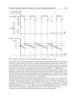
negligible values of the mean squares pure error, defines the simulation run length. Figure 8
shows the MS
PE
curve of distribution centre #2 that takes the greatest simulation time. After
500 days the MS
PE
values are negligible and further prolongations of the simulation time do
not give significant experimental error reductions.
Choosing for each simulation run the length evaluated by means of MS
PE
analysis (500
days), the validation phase is conducted using the Face Validation (informal technique). For
each retailer and for each distribution centre the simulation results, in terms of fill rate, are
compared with real results. For a better understanding of the validation procedure, let us
consider the store #1. Figure 9 shows six different curves, each one reporting the store

Supply Chain Management Based on Modeling & Simulation: State of the Art and
Application Examples in Inventory and Warehouse Management

115

Fig. 8. Mean Square Pure Error Analysis and Simulation Run Length
#1 fill rate versus time (days). In the graphs there is one real curve and five simulated curves
(note that during the validation process the simulation model works under identical input
conditions of the real supply chain).


Fig. 9. Main effects plot: Store #1 fill rate versus inventory control policies, lead time,

demand intensity and demand variability
Supply Chain Management

116
The plot is then shown to the supply chain’s experts asking them to make the difference
between the real curve and the simulated curves on the basis of their estimates (obviously
showing all the curves without identification marks). In our case the experts were not able to
see any difference between real and simulated curves, assessing (as consequence) the
validation of the simulation model. The Face Validation technique has been applied for the
remaining stores as well as for each distribution centre. Further results in terms of fill rate
confidence intervals have been analyzed. We concluded that, in its domain of application,
the simulation model recreates with satisfactory accuracy the real supply chain.
4. Experimental design, simulation runs and analysis
The first application example (proposed in this section) is a focus on the inventory problem
within the three-echelon stochastic supply chain presented above. The supply chain simulation
model is used for investigating a comprehensive set of operative scenarios including the four
different inventory control policies (discussed in section 3.2) under customers’ demand
intensity, customers’ demand variability and lead times constraints. The application example
also shows simulation capabilities as enabling technology for supporting decision-making in
supply chain management especially when combined with Design of Experiment, DOE, and
Analysis of Variance, ANOVA for simulation results analysis.
In this application example, nine stores, four distribution centers, three plants and twenty
items form the supply chain scenario. Before getting into simulation results details, let us
give some information about the simulation model efficiency in terms of time for executing
a simulation run. Each 500 days replication takes about one minutes (running on a typical
commercial desktop computer). If the number of replications is three, a simulation run is
over in 3 minutes. Our experience with supply chain simulation models developed using
eM-Plant (Longo, 2005a, 2005b), suggests simulation times higher then 10 minutes if the
traditional modeling approach is selected. Having obtained such times is not difficult to
carry out complete design of experiments using the full factorial experimental design.

Let us consider for each supply chain node four different parameters: the inventory control
policy, the lead time, the market demand intensity and the market demand variability and
let us call these parameters factors (in literature factors are also called treatments). In this
study, we have chosen, for each factor, different number of levels as reported in table 4.

Factors Levels
Inventory Control Policy (x
1
) rR,1 rR,2 rR,3 rR,4
Stores Lead Time (x
2
) 1 3 5
Customers’ Demand Intensity (x
3
) Low Medium High
Customers’ Demand Variability (x
4
) Low Medium High
Table 4. Factors and Levels
Note that the simulation model user can easily define a different supply chain scenario by
changing the number of echelons, the number of STs, DCs and PLs, the number of items or
select different parameters (i.e. demand forecast methodologies, transportation modalities,
priority rules for ordering and deliveries, etc.). Analogously new parameters or supply
chain features can be easily implemented thanks to simulator architecture completely based
on programming code. The objective of the application example is to understand the effects
of factors levels on three performance measures: fill rate (Y
1
), average on hand inventory
Supply Chain Management Based on Modeling & Simulation: State of the Art and
Application Examples in Inventory and Warehouse Management

117
(Y
2
) and inventory costs (Y
3
). The outcomes are input-output analytical relations (called the
meta-models of the simulation model).
In our application example, checking all possible factors levels combinations (full factorial
experimental design) requires 108 simulation runs; if each run is replicated three times we
have 324 replications. Having set the simulation model for executing three replications for
each simulation run and considering all the factors levels combinations, we have executed,
on a single desktop computer, all the experiments taking less than 6 hours. Note that, very
often, pre-screening analyses reduce the number of factors to be considered as well as
fractional factorial designs reduce the total number of simulation runs. The efficiency of the
simulation model in terms of time for executing simulation runs is largely due to the
simulation model architecture and modeling approach.
Monitoring the performance of an entire supply chain requires the collection of a huge
amount of simulation results. To give the reader an idea of the simulation results generated
by the simulation model in our application example, let us consider the fill rate: the
simulation model evaluates the fill rate at the end of each replication, as mean value over
500 days. For each supply chain node (both STs and DCs) and for each simulation run (a
single combination of the factors levels) the model evaluates 3 fill rate values (9 stores x 4
DCs x 109 simulation runs x 3 replications = 11772 values). Consider the average on hand
inventory: the simulation model evaluates, at the end of each replication, the mean value
over 500 days. For each supply chain node, for each simulation run and for each item, 3
values of the performance measures are collected (9 stores x 4 DCs x 109 simulation runs x 3
replications x 20 items =235440 values). The same number of values are automatically
collected for inventory costs. Obviously it is out of the scope of this chapter to report all
simulation results; some simulation results are reported and discussed to provide the reader

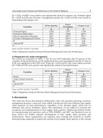
with a detailed overview of the proposed approach. Table 5 consists of some simulation
results for store #1 in terms of fill rate, average on hand inventory and inventory costs (only
for three of twenty items). The simulation results consider all factors levels combinations
keeping fixed the inventory control policy (rR1). The complete analysis consider 108
simulation runs for checking all factors levels combinations both for stores and DCs. The
huge number of simulation results has required the implementation of a specific tool for
supporting output analysis. To this end eM-Plant is jointly used with Microsoft Excel and
Minitab. As before mentioned, at the end of each replication, simulation results are
automatically stored in Excel spreadsheets. Visual Basic Macros are implemented and used
for performance measures calculation. Such values are then imported in Minitab projects
(opportunely set with the same design of experiments) for statistic analysis. The Microsoft
Excel interface works correctly in each supply chain scenario (not only in the application
example proposed). The results in terms of mean values calculated by the Microsoft Excel
interface can be analyzed by using plots and charts (i.e. fill rate versus inventory policies, on
hand inventory versus lead time, etc.). The use of the simulation model does not necessarily
require DOE , ANOVA or any kind of statistical methodologies or software.
4.1 Simulation results analysis and input output meta-models
Table 5 reports some simulation results for store #1. Let us give a look to the fill rate: the
higher is the demand intensity and variability the lower is the fill rate. Such behavior could
be explained by considering a greater error in lead time demand (demand forecast over the
lead time) as well as a greater number of stock outs and unsatisfied orders. A three-day lead
time performs better (in terms of fill rate) than one-day lead time. In addition the higher is
Supply Chain Management

118
the demand intensity and demand variability the lower is the average on hand inventory
(see items 1, 2, 3 in table 5, remaining items show a similar behavior). The higher is the lead
time the higher is the average on hand inventory. In effect the higher demand intensity
causes an inventory reduction (due to the higher number or orders) whilst a five-day lead
time causes high values of the lead time demand. The qualitative explanation of inventory

cost seems to be more difficult because of the interaction among the different factors levels.
It is worth say that a qualitative description or analysis of simulation results does not
provide a deep understanding of the supply chain behavior and could lead to erroneous
conclusions in the decision making process. We know that experiments are natural part of
the engineering and scientific process because they help us in understanding how systems
and processes work. The validity of decisions taken after an experiment strongly depends
on how the experiment was conducted and how the results were analyzed. For these
reasons, we suggest to use the simulation model jointly with the Design of Experiment
(DOE) and the Analysis of Variance (ANOVA): DOE for experiments planning and ANOVA
for understanding how factors (input parameters) affect the supply chain behavior. In effect,
many definitive simulation references (i.e. Banks, 1998) say that if some of the processes
driving a simulation are random, the output data are also random and simulation runs
result in estimates of performance measures. In other words, specific statistical techniques
(i.e. DOE and ANOVA) could provide a good support for simulation results analysis.
Our treatment uses ANOVA for understanding the impact of factors levels on performance
measures. Let Y
k
be one of the performance measures previously defined (k = 1, 2, 3), let x
i

be the factors or treatments (with x
i
varying between the levels specified in table 4), let β
ij
be
the coefficients of the model and let hypothesize a linear statistic input-output model to
express Y
k
as function of x
i

.

0, , , , , , , , , ,
1
,,, , ,
jh
kk
j
k
j
ki
j
kik
j
ki
j
mk ik
j
kmk
jij ijm
ijmnk ik jk mk nk k
ijmn
Y x xx xxx
xxx x
ββ β β
βε
=
=< <<
<< <
=+ + + +

++
∑∑∑ ∑∑∑
∑∑∑ ∑
(14)
k = 1, 2, 3 number of performance measures;
h = 1, 2, 3, 4 number of factors.
The Analysis of Variance allows to evaluate those factors that have a real impact on the
performance measure considered or, in other words, evaluating all the terms in equation
(14) eventually deleting insignificant factors from the input-output model. The Analysis of
Variance decompose the total variability of
Y
k
into components; each component is a sum of
squares associated with a specific source of variation (treatments) and it is usually called
treatment sum of squares. Without enter in formulas details, if changing the levels of a
factor has no effect on
Y
k
variance, then the expected value of the associated treatment sum
of squares is just an unbiased estimator of the error variance (this is known as null
hypothesis, H
0
).
On the contrary, if changing the level of a factor has effect on
Y
k
,

then the expected value of the
associated treatment sum of squares is the estimation of the error plus a positive term that

incorporates variation due the effect of the factor (alternative hypothesis, H
1
). It follows that,
by comparing the treatment mean square and the error mean square, we can understand
which factors affect the performance measure Y
k
. Such comparison is usually made by using a
Fisher-statistic test. In addition, the ANOVA evaluates the coefficients of equation 14.
Supply Chain Management Based on Modeling & Simulation: State of the Art and
Application Examples in Inventory and Warehouse Management

119
Inventory
Control
Policy
Lead
Time
Demand
Intensity
Demand
Variability
Run Order
Fill Rate
Average
OHI –
Item1
Average
OHI –
Item2
Average

OHI –
Item3
Inventory
Cost –
Item1 [€]
Inventory
Cost –
Item2 [€]
Inventory
Cost –
Item3 [€]
rR1
1
Low
Low
1
0,762
103
85
78
408,46
420,64
407,21
rR1
1
Low
Medium
2
0,728
104

84
79
524,02
562,90
520,22
rR1
1
Low
High
3
0,733
104
85
80
520,67
547,96
549,76
rR1
1
Medium
Low
4
0,536
37
36
34
790,32
754,04
692,61
rR1

1
Medium
Medium
5
0,533
38
36
35
770,76
749,73
696,53
rR1
1
Medium
High
6
0,525
37
36
35
766,29
727,03
691,30
rR1
1
High
Low
7
0,386
20

19
20
996,79
910,36
919,58
rR1
1
High
Medium
8
0,385
20
18
19
881,84
1039,74
985,23
rR1
1
High
High
9
0,374
21
19
20
891,43
921,24
873,29
rR1

3
Low
Low
10
0,838
112
95
89
441,44
447,90
436,59
rR1
3
Low
Medium
11
0,833
113
94
90
559,20
622,53
606,67
rR1
3
Low
High
12
0,813
113

95
90
568,77
602,89
578,57
rR1
3
Medium
Low
13
0,578
52
49
48
838,59
800,66
786,28
rR1
3
Medium
Medium
14
0,554
53
50
51
768,47
754,35
774,04
rR1

3
Medium
High
15
0,560
54
48
49
831,60
782,69
770,58
rR1
3
High
Low
16
0,402
36
34
45
1038,40
975,13
988,23
rR1
3
High
Medium
17
0,376
40

38
42
827,87
901,80
953,69
rR1
3
High
High
18
0,379
41
42
35
933,43
961,85
811,90
rR1
5
Low
Low
19
0,828
119
100
93
439,70
454,48
411,17
rR1

5
Low
Medium
20
0,837
118
101
95
579,33
618,32
581,03
rR1
5
Low
High
21
0,829
119
98
94
577,69
594,15
589,47
rR1
5
Medium
Low
22
0,561
55

57
51
794,86
833,73
714,95
rR1
5
Medium
Medium
23
0,581
58
56
58
785,19
852,77
808,67
rR1
5
Medium
High
24
0,568
57
56
53
793,25
871,55
710,71
rR1

5
High
Low
25
0,394
49
48
54
998,87
983,49
971,56
rR1
5
High
Medium
26
0,399
54
49
51
969,71
1019,55
952,16
rR1
5
High
High
27
0,399
48

49
42
952,87
990,75
1036,61

Table 5. Simulation results for Store #1 (rR1 inventory control policy, 3/20 items)
Supply Chain Management

120
Table 6 consists of some results obtained using the statistical software Minitab: the fill rate
ANOVA (table 6, upper part) and average on hand inventory ANOVA (table 6, lower part)
of item #1 for store #1. In addition, table 6 reports all the terms of equation 14 (for both
performance measures).
From the ANOVA theory it is well known that all the factors with a
p value less or equal to
the confidence level used for the analysis (α=0.05) have an impact on the performance
measure. The
P-value is the probability that the F-statistic test will take on a value that is at
least as extreme as the observed value of the statistic when the null hypothesis
H0 is true.
Let us discuss the results of the fill rate ANOVA reported in the upper part of table 6. Note
that all factors levels have an impact on the fill rate. All the effects have to be taken into
consideration: first order, second order, third order and fourth order effects. Such results
show the high complexity of a supply chain and the strong interaction among the control
policy used for inventory management and other critical factors such as demand intensity
and variability and lead times (usually in many systems the third and fourth effects can be
neglected).
For a better understanding of the fill rate analysis of variance (for store #1) we have plotted
(see figures 10 and 11) the main effects and the second order interaction effects of equation

(14). The inventory control policies have a different effect on store #1 fill rate.
rR1 and rR3
give as result an average fill rate of about 0.55 (mostly showing an analogous behavior);
rR2gives an average fill rate of about 0.40 (the worst performance) and rR4 about 0.60 (the
best one). The rR4 policy performs better than the other policies because it uses the policy
parameters review period is based on cost optimization. The demand intensity has a strong
impact on fill rate due to the greater number of required items: the average fill rates is about
0.80 in correspondence of low demand intensity, 0.50 in correspondence of medium
intensity and 0.35 in case of high intensity. Lead times and demand variability cannot be
considered as important as inventory control policy and demand intensity even if their
effect on fill rate cannot be neglected.
Now let us focus on interaction effects (see fig. 11). The interaction between inventory
control policies and lead times show a better behavior for rR1 and rR2 in correspondence of
high lead times (the average fill rate increases in correspondence of higher lead times from
0.5 to 0.6 for rR1 policy and from 0.25 to 0.40 for rR2 policy). On the contrary, rR3 and rR4
show an opposite behavior and perform better with low lead-time values: the average fill
rate decreases from 0.65 to 0.50 for rR3 policy and from 0.65 to 0.60 for rR4 policy. Note that
the fill rate reduction with rR4 is smaller than the reduction with rR3. With regards to
demand intensity rR1, rR3, rR4 policies show a similar trend in correspondence of low,
medium and high demand intensity (the fill rate decrease from 0.90 to 0.40), whilst rR2 gives
lower fill rate values (from 0.60 to 0.20). Similar results emerge when considering demand
variability: rR1, rR3, rR4 policies show a similar trend (fill rate around 0.60 even if the rR4
performs better than rR1 and rR3), whilst rR2 gives the worst performance (fill rate about
0.40). All the remaining plots in figure 10 give useful information as well as help in
understanding how the interaction among factors levels affect the store fill rate.
Both first order effect plots (figure 10) and interaction plots (figure 11) are obtained by using
equation 14. The
Terms columns (upper part of table 6) report all the values of the
coefficients of equation 14. Such coefficients must be read per column and their order
reflects the order of the experimental design matrix (i.e. consider the performance measure

fill rate,
Y
1
, β
01
=0.0022, β
11
=-0.0010, etc.). Focusing only on fill rate, the best design solution
for store #1 is rR4 inventory control policy and three days lead time.
Supply Chain Management Based on Modeling & Simulation: State of the Art and
Application Examples in Inventory and Warehouse Management

121
Fill rate ANOVA – Store #1
Source
DF
Seq SS
Adj SS
Adj MS
F
P
Terms
Terms
Terms
Terms
Terms
Terms
Terms
x
1

3
2,87475
2,87475
0,95825
5832,04
0,000
0,7185
0,0022
-0,0054
-0,0253
-0,0113
0,0051
0,0148
x
2

2
0,07717
0,07717
0,03858
234,83
0,000
0,0314
-0,0010
-0,0051
-0,0082
-0,0084
-0,0082
0,0159

x
3

2
11,07926
11,07926
5,53963
33714,93
0,000
-0,1575
-0,0288
0,0115
-0,0107
0,0065
-0,0034
-0,0258
x
4

2
0,01681
0,01681
0,00841
51,16
0,000
0,0335
-0,0158
0,0112
0,0046
0,0022

0,0072
-0,0254
x
1
*x
2

6
0,41302
0,41302
0,06884
418,95
0,000
-0,0192
0,0409
-0,0058
0,0057
0,0054
0,0167
0,0132
x
1
*x
3

6
0,18962
0,18962
0,0316
192,34

0,000
0,0185
-0,0005
-0,0060
-0,0068
0,0017
-0,0016
0,0107
x
1
*x
4

6
0,03237
0,03237
0,00539
32,83
0,000
0,2402
-
0,0052
0,0016
-0,0017
0,0070
-0,0082

x
2
*x

3

4
0,13543
0,13543
0,03386
206,07
0,000
-0,0306
-0,0051
0,0069
0,0028
0,0033
0,0113

x
2
*x
4

4
0,0231
0,0231
0,00577
35,15
0,000
0,0057
-0,0014
-0,0040
-0,0003

0,0034
0,0133

x
3
*x
4

4
0,04209
0,04209
0,01052
64,05
0,000
0,0044
0,0096
0,0107
0,0290
0,0086
-0,0094

x
1
*x
2
*x
3

12
0,19436

0,19436
0,0162
98,58
0,000
-0,0139
0,0142
-0,0593
0,0226
0,0025
-0,0022

x
1
*x
3
*x
4

12
0,07523
0,07523
0,00627
38,16
0,000
-0,0036
-0,0309
0,0284
-0,0140
0,0036
0,0113

x
2
*x
3
*x
4

8
0,05234
0,05234
0,00654
39,82
0,000
-0,0555
-0,0016
0,0113
-0,0114
-0,0126
0,0044

x
1
*x
2
*x
4

12
0,08415

0,08415
0,00701
42,68
0,000
-0,0005
0,0172
-0,0012
-0,0068
-0,0139
-0,0049

x
1
*x
2
*x
3
*x
4

24
0,16346
0,16346
0,00681
41,45
0,000
0,0460
-0,0134
0,0271
-0,0090

-0,0146
-0,0014

Error
216
0,03549
0,03549
0,00016


0,0239
-0,0026
-0,0337
0,0030
-0,0141
-0,0274

Total
323
15,48867




-0,0196
-0,0034
0,0091
0,0059
0,0134
-0,0299

Item #1 on hand inventory ANOVA – Store #1
Source
DF
Seq SS
Adj SS
Adj MS
F
P
Terms
Terms
Terms
Terms
Terms
Terms
Terms
x
1

3
115183,2
115183,2
38394,4
6738,78
0,000
75,8025
1,3951
-0,3272
-0,1759
-0,6728

1,8395
0,4722
x
2

2
29430,7
29430,7
14715,3
2582,76
0,000
-15,7284
3,9012
-0,4846
-0,9136
-0,4599
-0,3549
1,4167
x
3

2
199587,1
199587,1
99793,5
17515,22
0,000
-20,5679
1,8642
0,2469

-0,3210
0,5216
-1,1142
-1,5370
x
4

2
105,2
105,2
52,6
9,23
0,000
11,3333
-11,8519
0,1728
0,1790
0,2068
1,3025
-1,2315
x
1
*x
2

6
674,7
674,7
112,5
19,74

0,000
-12,5617
3,1481
-0,3642
0,8272
-0,0895
-0,2068
1,3796
x
1
*x
3

6
10050,3
10050,3
1675
293,99
0,000
2,0494
0,4321
-0,1605
-0,8272
0,5864
0,4043
-0,0093
x
1
*x
4

6
138,8
138,8
23,1
4,06
0,001
34,8642
-0,1327
-0,4506
-0,3086
0,0679
-0,2438

x
2
*x
3

4
2924,1
2924,1
731
128,31
0,000
-13,9136
-
0,2840
0,3920
0,3765

0,2994
1,1790

x
2
*x
4

4
92,2
92,2
23,1
4,05
0,003
-0,8025
-0,5525
-0,9043
0,5062
0,1821
-0,0617

x
3
*x
4

4
26,1
26,1
6,5

1,15
0,336
0,4660
0,3704
0,0216
2,8148
0,3395
-0,7747

x
1
*x
2
*x
3

12
995,3
995,3
82,9
14,56
0,000
-0,1420
0,9537
-1,3642
0,8148
-0,4012
-0,1265

x

1
*x
3
*x
4

12
426,2
426,2
35,5
6,23
0,000
0,7284
4,3395
-0,0772
-1,0185
0,8673
0,8457

x
2
*x
3
*x
4

8
236,3
236,3
29,5

5,18
0,000
3,0309
0,4228
-0,7809
-1,0741
-0,6574
0,7438

x
1
*x
2
*x
4

12
469,9
469,9
39,2
6,87
0,000
-1,1358
-0,2438
0,4784
-0,3395
-1,4630
-0,1636

x

1
*x
2
*x
3
*x
4

24
786,6
786,6
32,8
5,75
0,000
-0,5741
0,2006
3,5370
-0,5432
-0,6481
0,0401

Error
216
1230,7
1230,7
5,7


-0,5556
0,2006

-1,3241
0,7994
-1,1204
-2,0556

Total
323
362357,4




2,0988
-0,2901
2,1574
0,4846
0,3765
-2,0000


Table 6. Analysis of Variance for Store #1 (
Fill Rate and item#1 Average On Hand Inventory)
and equation 14 coefficients
Supply Chain Management

122
Let us consider now the analysis of variance of the average on hand inventory for store #1
and item #1 (lower part of table 6). All the factors have an impact on the average on hand
inventory except for the interaction x3*x4 (Demand Intensity and Demand Variability). The
lower right part of table 6 consists of terms of equation (14). Also in this case the equation 14

can be used for plotting first order and interaction effects and understanding, from a
quantitative point of view, the average on hand inventory behavior.
Needless to say that similar results have been obtained for the third performance measure,
the inventory cost. The same approach is followed for each item of store #1, for each store
and for each distribution center. Note that the aim of the application example is not to find
out the best configuration of the supply chain but to show the complexity of the inventory
problem along the supply chain and the simulation potentials as decision-making tool for
supply chain management. The high level of results detail (analysis of the fill rate for each
supply chain node, analysis of on hand inventory and inventory costs for each item and in
each supply node) helps in understanding simulation models capabilities as decision-
making tool. In effect as reported in literature (refer to literature overview section) the
supply chain decision process requires accurate analysis on the whole supply chain. In
addition, the simulation model architecture jointly with Excel and Minitab spreadsheets
guarantees high flexibility in terms of supply chain scenarios definition, high efficiency in
terms of time for executing simulation runs and analyzing simulation results.


Fig. 10. Main effects plot: Store #1 fill rate versus inventory control policies, lead time,
demand intensity and demand variability
Supply Chain Management Based on Modeling & Simulation: State of the Art and
Application Examples in Inventory and Warehouse Management

123

Fig. 11. Effects of factors interaction on fill rate
4.2 Testing the simulation results validity: residuals analysis
In using ANOVA for simulation results analysis, we strongly suggest to test ANOVA results
validity. The Analysis of Variance assumes (as starting hypothesis) that the observations are
normally and independently distributed, with the same variance for any combination of
factors levels. These assumptions must be verified by means of the analysis of residuals for

accepting the validity of the input-output analytical models (equation 14).
A residual is the difference between an observation of the performance measure and the
corresponding average value calculated on the 3 replications. The assumption of normality
can be tested by building a
normal probability plot of residuals. If residuals approximately fall
along a straight line passing form the centre of the graph, the assumption of normality can
be accepted. In figure 12 (upper-left part) we observe that the deviation from normality is
not severe (store #1, fill rate). The assumption of equal variance is tested by plotting
residuals against the factors levels or against the fill rate: residuals variability must anyhow
not depend on the level of factors or on the fill rate. Figure 12 (upper-right part) shows
residuals versus the fitted values and do not show any particular trend; therefore, the equal
variance hypothesis is accepted. Finally, the assumption of independence is tested by
plotting residuals against the implementation order of simulation runs. A sequence of
positive or negative residuals could indicate that observations are dependent among
themselves. Figure 12 (lower part) shows that the hypothesis of independence of
observations is accepted. The residuals analysis, as part of the Minitab standard tools, can be
easily carried out for each supply chain scenario.
In case of starting hypothesis rejection, a linear statistical model (as the model in equation
14) must be rejected. A test for model curvature should be conducted.
Supply Chain Management

124

Fig. 12. Test of the simulation results validity: Residuals analysis
5. The Warehouse management problem: interactions among operational
strategies, available resources and internal logistic costs
The survey of state of art proposed in section 2.2 highlights that, very often, models
proposed are not able to recreate the whole complexity of a real warehouse system
(including stochastic variables, huge number of items, multiple deliveries, etc). The
application example proposed in this section investigates the effects of warehouse resources

management on warehouse efficiency highlighting as the interactions among operational
strategies and available resources strongly affect the internal logistic costs. In particular the
simulation model of a real warehouse is presented. The simulator, called WILMA
(
Warehouse and Internal Logistics Management) has been developed under request of one of
the major Italian company operating in the large scale retail sector.
5.1 Warehouse description and warehouse simulation model
As before mentioned, the warehouse belongs to one of the most important company
operating in the large scale retail sector (in Italy) and it is characterized by:
• total surface: 13000 m
2
;
• shelves surface: 5000 m
2
;
• surface for packing and shipping operations: 3000 m
2
;
• surface for unloading and control operations: 1800 m
2
;
• three levels of shelves;
• eight types of products;
• capacity in terms of pallets: 28400 pallets;
Supply Chain Management Based on Modeling & Simulation: State of the Art and
Application Examples in Inventory and Warehouse Management

125
• capacity in terms of pallets for each product: 3550 pallets;
• capacity in terms of packages: about one million packages.

Figure 13 shows the warehouse layout.


Fig. 13. The warehouse layout
The main modeling effort was carried out to recreate with satisfactory accuracy the most
important warehouse operations:
• trucks arrival and departure for items deliveries (from suppliers to the warehouse and
from the warehouse to retailers);
• materials handling operations (performed by using forklifts and lift trucks) including,
trucks unloading operations, inbound quality and quantity controls, preparation for
storage, storage operations, retrieval operations, picking operations, preparation for
shipping, packaging operations, trucks loading operations and shipping;
• performance measures control and monitoring (a detailed description of performance
measures will be provided later on).
The simulation software adopted for developing WILMA simulator is the commercial
package Anylogic™ by
XJ Technologies. Most of the logics and rules of the real warehouse
are implemented by using ad-hoc Java routines. The description proposed below will be
useful for those readers interested in developing similar simulation models. Figure 14 shows
the simulation model Flow Chart.
In order to support scenarios investigation, the main variables of the WILMA simulator
have been completely parametrized. To this end, the simulator is equipped with a dedicated
Graphic User Interface (GUI) with a twofold functionality:
• to increase the simulation model flexibility changing its input parameters both at the
beginning of the simulation run and at run-time observing the effect on the warehouse
behavior (
Input Section);
• to provide the user with all simulation outputs for evaluating and monitoring the
warehouse performances (Output Section).
Supply Chain Management

126

Fig. 14. The WILMA Simulation Model Flow Chart
The
Input Section (figure 15) is in four different parts:
• The Suppliers’ Trucks section which includes slider objects for changing the following
parameters: suppliers’ trucks arrival time, number of suppliers’ trucks per day, time
window in which suppliers’ trucks deliver products;
• the Retailers’ Trucks section includes slider objects for changing the following
parameters: retailers’ trucks arrival time, number of retailers’ trucks per day, time
window for retailers’ trucks arrival, time for starting items preparation;


Fig. 15. The WILMA Input Section (part of the WILMA Graphic User Interface)
Supply Chain Management Based on Modeling & Simulation: State of the Art and
Application Examples in Inventory and Warehouse Management

127
• the Warehouse Management parameters section which includes slider objects for changing
the following parameters: shelves levels, number of forklifts, number of lift trucks,
number of docks available for loading and unloading operations, forklifts and lift trucks
efficiency, stock-out costs parameters;
• the Logistics Internal Costs section which includes slider objects for changing the
following parameters: sanction fee for retailers/suppliers, time after which the
warehouse has to pay a sanction fee to retailers for operations performed out of the
scheduled period, time after which suppliers have to pay a sanction fee to the
warehouse for operations performed out of the scheduled period.
The
Output Section (figure 16) provides the user with the most important warehouse

performance measures. The main performance measures include the following:
• forklifts utilization level;
• lift trucks utilization level;
• service level provided to suppliers’ trucks;
• service level provided to retailers’ trucks;
• waiting time of suppliers’ trucks before starting the unloading operations;
• waiting time of retailers’ trucks before starting the loading operations;
• number of packages handled per day (actual and average values);
• daily cost for each handled package (actual and average values).


Fig. 16. The WILMA Output Section (part of the WILMA Graphic User Interface)
5.2 Internal logistics management: scenarios definition and simulation experiments
The WILMA simulation model has been used to investigate the effects of warehouse
resources management on warehouse efficiency highlighting as the interactions among
operational strategies and available resources strongly affect the internal logistic costs. The
analysis carried out by using the WILMA simulator include the following:
• internal resources allocations versus number of packages handled per day;
• internal resources allocations versus the daily cost for each handled package;
• Internal resources allocations versus suppliers’ waiting time and retailers’ waiting time
In each case a sensitivity analysis is carried out and an input-output analytical model is
determined. As in the first application example, the simulation approach is jointly used with
the Design of Experiments and Analysis of Variance.
Supply Chain Management

128
The input parameters (
factors) taken into consideration are:
• the number of suppliers’ trucks per day (NTS);
• the number of retailers’ trucks per day (NTR);

• the number of forklifts (NFT);
• the number of lift trucks (NMT);
• the number of shelves levels (SL).
The variation of such parameters creates distinct operative scenarios characterized by
different operative strategies and resources availability, allocation and utilization. The
performance measures considered are:
• the average number of handled packages per day (APDD);
• the average value of the daily cost for each handled package (ADCP);
• the waiting time of suppliers’ trucks before starting unloading operations (STWT);
• the waiting time of retailers’ trucks before starting loading operations (RTWT).
The experiments planning is supported by the Design of Experiments (a Full Factorial
Experimental Design is used). Table 7 consists of factors and levels used for the design of
experiments.

Factors Level 1 Level 2
Number of suppliers’ trucks per day, NTS (x
1
) 80 100
Number of retailers’ trucks per day, NTR (x
2
) 30 40
Number of forklifts, NFT, (x
3
) 6 24
Number of lift trucks, NMT, (x
4
) 12 50
Number of shelves levels, SL, (x
5
) 3 5

Table 7. DOE Factors and Levels
As shown in Table 7, each factor has two levels: in particular, Level 1 indicates the lowest
value for the factor while Level 2 its greatest value. In order to test all the possible factors
combinations, the total number of the simulation runs is 2
5
. Each simulation run is
replicated three times, so the total number of replications is 96 (32x3=96). The simulation
results are studied, according to the various experiments, by means of the Analysis Of
Variance (
ANOVA) and graphic tools.
Let Y
i
be the i-th performance measure and let x
i
be the factors, equation 15 expresses the i-th
performance measure as linear function of the factors.

555 555 5555
0
11 1 1
555 5 5
1
i i i ij i j ijh i j h ijhk i j h k
i i ji i jihj i jihjkh
ijhkp i j h k p ijhkpn
ijihjkhpk
Yxxx xxx xxxx
xxx x x
ββ β β β
βε

==> =>> =>>>
=>>> >
=+ + + + +
++
∑∑∑ ∑∑∑ ∑∑∑∑
∑∑∑∑ ∑
(15)

where:

0
β
is a constant parameter common to all treatments;
Supply Chain Management Based on Modeling & Simulation: State of the Art and
Application Examples in Inventory and Warehouse Management

129
5
1
ii
i
x
β
=
∑
are the five main effects of factors;

55
1
i

j
i
j
iji
xx
β
=>
∑∑
are the ten two-factors interactions;

555
1
i
j
hi
j
h
ijihj
xxx
β
=>>
∑∑∑
represents the three-factors interactions;

555 5
1
i
j
hk i
j

hk
ijihjkh
xxx x
β
=>>>
∑∑∑∑
are the three four-factors interactions;

555 5 5
1
i
j
hk
p
i
j
hk
p
ijihjkhpk
xxx x x
β
=>>> >
∑∑∑∑ ∑
is the sole five-factors interaction;
ε
ijhkpn
is the error term;
n is the number of total observations.
In particular the analysis carried out aims at:
• identifying those factors that have a significant impact on the performance measures

(sensitivity analysis);
• evaluating the coefficients of equation 4.2 in order to have an analytical relationship
capable of expressing the performance measures as function of the most critical factors.
5.3 Internal resources allocations versus number of packages handled per day
(APDD)
Table 8 reports the experiments design matrix and the simulation results in terms of average
number of handled packages per day. The first four table columns show all the possible
combinations of the factors levels while the last column reports the results provided by the
WILMA simulation model for the APDD performance measure. Note that the APDD values
reported in the last column of Table 8 are values obtained as average on three simulation
replications.
According to the ANOVA theory, the non-negligible effects are characterized by
p-value ≤ α
where p is the probability to accept the negative hypothesis (the factor has no impact on the
performance measure) and α = 0.05 is the confidence level used in the analysis of variance.
According to the ANOVA, the most significant factors are:
• NTS (the number of suppliers’ trucks per day);
• NTR (the number of retailers’ trucks per day);
• NFT (the number of forklifts);
• NMT (the number of lift trucks);
• NTR*NMT (the interaction between the number of retailers’ trucks per day and the
number of lift trucks);
• NTS* NTR* NFT (the interaction between the number of suppliers’ trucks per day, the
number of retailers’ trucks per day and the number of forklifts).
Supply Chain Management

130
NTS NTR NFT NMT SL APDD
80 30 6 12 3 30370
80 30 6 12 5 30345

80 30 6 50 3 30439
80 30 6 50 5 30457
80 30 24 12 3 30421
80 30 24 12 5 30358
80 30 24 50 3 30387
80 30 24 50 5 30488
80 40 6 12 3 40574
80 40 6 12 5 40501
80 40 6 50 3 40603
80 40 6 50 5 40580
80 40 24 12 3 40551
80 40 24 12 5 40568
80 40 24 50 3 40553
80 40 24 50 5 40541
100 30 6 12 3 38528
100 30 6 12 5 37181
100 30 6 50 3 30361
100 30 6 50 5 30399
100 30 24 12 3 30388
100 30 24 12 5 30405
100 30 24 50 3 30416
100 30 24 50 5 30387,6
100 40 6 12 3 35846,1
100 40 6 12 5 37186,2
100 40 6 50 3 40498,8
100 40 6 50 5 40532,1
100 40 24 12 3 40550
100 40 24 12 5 35447,4
100 40 24 50 3 40530
100 40 24 50 5 40563,6

Table 8. Design Matrix and Simulation Results (APDD)
ANOVA results are summarized in table 9:
• the first column reports the sources of variations;
• the second column is the degree of freedom (DOF);
• the third column is the Sum of Squares;
• the 4
th
column is the Adjusted Mean Squares;
• the 5
th
column is the Fisher statistic;
• the 6
th
column is the p-value.

Source DOF AdjSS AdjMS F P
Main Effects 4 50,30 125,75 23,22 0
2-Way interactions 1 45,24 4,52 8,35 0
3-Way interactions 1 24,84 2,48 4,59 0,04
Residual Error 25 13,53 0,54
Total 31
Table 9. ANOVA Results for APDD (most significant factors)
Supply Chain Management Based on Modeling & Simulation: State of the Art and
Application Examples in Inventory and Warehouse Management

131
The input-output meta-model expressing APDD as function of the most important factors is
the following:

21777 21, 46 * 348,74 * 167,083 *

423,71 * 12,51 * ( * ) 0,028 * ( * * )
APDD NTS NTR NFT
NMT NTR NMT NTS NTR NFT
=
++ − +
−+ +
(16)

Equation 16 is the most important result of the analysis: it is a powerful tool that can be used
for correctly defining, in this case, the average number of packages handled per day in
function of the warehouse available resources.
5.4 Internal resources allocations versus the daily cost for each handled package
(ADCP)
The same analysis is carried out taking into consideration the average daily cost per handled
packages (ADCP). Table 10 reports the design matrix and the simulation results. The normal

NTS NTR NFT NMT SL ADCP
80 30 6 12 3 1,38
80 30 6 12 5 1,33
80 30 6 50 3 0,48
80 30 6 50 5 0,483
80 30 24 12 3 3,06
80 30 24 12 5 3,91
80 30 24 50 3 2,27
80 30 24 50 5 0,623
80 40 6 12 3 1,38
80 40 6 12 5 13,82
80 40 6 50 3 0,45
80 40 6 50 5 11,54
80 40 24 12 3 4,69

80 40 24 12 5 5,3
80 40 24 50 3 3,69
80 40 24 50 5 2,89
100 30 6 12 3 3,05
100 30 6 12 5 4,31
100 30 6 50 3 0,53
100 30 6 50 5 6,72
100 30 24 12 3 5
100 30 24 12 5 6,28
100 30 24 50 3 0,64
100 30 24 50 5 0,62
100 40 6 12 3 3,72
100 40 6 12 5 8,18
100 40 6 50 3 1,06
100 40 6 50 5 8,97
100 40 24 12 3 2,7
100 40 24 12 5 11
100 40 24 50 3 0,48
100 40 24 50 5 0,47
Table 10. Design Matrix and Simulation Results (ADCP)
Supply Chain Management

132
probability plot in Figure 17 allows to evaluate the predominant effects (red squares): in this
case the first order effects and some effects of the second order:
• NTR (the number of retailers’ trucks per day);
• NMT (the number of lift trucks);
• SL (the number of shelves levels);
• NTR*SL (the interaction between the number of retailers’ trucks per day and the
number of shelves levels);

• NFT*SL (the interaction between the number of suppliers’ trucks per day and the
number of shelves levels).




Fig. 17. The Most Significant Effects for the ADCP
Figure 18 shows the trend of ADCP in function of the main effects NTR, NMT and SL. As
reported in Figure 18, when the number of lift trucks increases, the average daily cost for
packages delivered decreases; the contrary happens with the shelves levels and the number
of retailers’ trucks variations.
Finally, Figure 19 presents the plots concerning the interaction effects between some couples
of parameters (i.e NTR-NFT, NFT-SL). The results obtained by means of DOE and ANOVA
allow to correctly arrange warehouse internal resources in order to maximize the average
number of handled packages per day and to minimize the total logistics internal costs. In
effect an accurate combination of the number of forklifts and lift trucks, help to keep under
control both the number of handled packages per day and the total logistic costs.
Supply Chain Management Based on Modeling & Simulation: State of the Art and
Application Examples in Inventory and Warehouse Management

133

Fig. 18. ADCP versus Main Effects


Fig. 19. Interactions Plots for the ADCP
Supply Chain Management

134
5.5 Internal resources allocations versus suppliers’ waiting time (STWT) and retailers’

waiting time (RTWT)
This Section focuses on evaluating the analytical relationship between factors defined in
Table 7 and the waiting time of suppliers’ trucks before starting the unloading operation
and the waiting time of retailers’ trucks before starting the loading operation. Such
relationships should be used for a correct system design.
The first analysis carried out aims at detecting factors that influence the waiting time of
suppliers’ trucks before starting the unloading operations (
STWT). Adopting also in this
case a confidence level α = 0.05, the Pareto Chart in Figure 20 highlights factors that
influence STWT. These factors are:
• the number of retailers’ trucks per day (NTR);
• the number of shelves levels (SL);
• the interaction factor between NTR and SL (NTR*SL).

Term
Standardized Effect
ADE
BCD
AE
A
AD
ABD
CD
AB
ABE
CDE
DE
BDE
BD
AC

ACE
ACD
BCE
ABC
D
BC
C
CE
BE
B
E
3,53,02,52,01,51,00,50,0
2,447
A
B
C
D
E
Factor
Pareto Chart of the Standardized Effects
(response is STWT, Alpha = ,05)
NTS
NTR
NFT
NMT
SL

Fig. 20. The Pareto Chart for the STWT
Repeating the ANOVA for the most important factors, it is confirmed that factors are correctly
chosen because their p-value is lower than the confidence level, as reported in Table 4.V.

Source DF AdjSS AdjMS F P
Main Effects 2 14,38 7,19 8,26 0,002
2-Way interactions 1 5,34 5,34 6,14 0,02
Residual Error 28 24,39 0,871
Total 31
Table 11. ANOVA Results for STWT
The input-output meta-model which expresses the analytical relationship between the
STWT and the most significant factors is reported in equation 17.
Supply Chain Management Based on Modeling & Simulation: State of the Art and
Application Examples in Inventory and Warehouse Management

135

713,58 24,19 * 234,32 * 8,17 *( * )STWT NTR SL NTR SL
=
−−++ (17)
This equation clearly explains how the waiting time of suppliers’ trucks before starting the
unloading operations depends on warehouse available resources.
The same analysis has been carried out taking into consideration the waiting time of retailers’
trucks before starting loading operations (
RTWT). Figure 21 (Normal Probability Plot of the
Standardized Effects) helps in understanding those factors that have a significant impact on
RTWT; in this case the first order effects and some effects of the second and third order:
• the number of retailers’ trucks per day (NTR);
• the number of lift trucks (NMT);
• the number of shelves levels (SL);
• the interaction factor between NTS and NTR (NTS*NTR);
• the interaction factor between NTS and NFT (NTS*NFT);
• the interaction factor between NTR and SL (NTR*SL);

• the interaction factor between NFT and NMT (NFT*NMT);
• the interaction factor between NFT and SL (NFT*SL);
• the interaction factor between NTR, NFT and SL (NTR*NFT*SL);
• the interaction factor between NFT, NMT and SL (NFT*NMT*SL).
Table 12 reports analysis of variance results while equation 18 is the input-output analytical
model that expresses RTWT as function of the predominant effects:
261,843 13,125 * 3,159 * 166,299 * 0,081 * ( * )
0,029 *( * ) 5,930 *( * ) 0,122 * ( * ) 1,027 * ( * )
0,073 *( * * ) 0,022 *( * * )
RTWT NTR NMT SL NTS NTR
NTS NFT NTR SL NFT NMT NFT SL
NTR NFT SL NFT NMT SL
=− + − + +
−++ ++
−−
(18)

Standardized Effect
Percent
5,02,50,0-2,5-5,0-7,5
99
95
90
80
70
60
50
40
30
20

10
5
1
A
B
C
D
E
Factor
Not Significant
Significant
Effect Type
CDE
BCE
CE
CD
BE
AC
AB
E
D
B
Normal Probability Plot of the Standardized Effects
(response is RTWT, Alpha = ,05)
NTS
NTR
NFT
NMT
SL

Fig. 21. The Normal Probability Plot for the RTWT