Advances in Spacecraft Technologies Part 15 doc

2 Advances in Spacecraft Technologies
It has been demonstrated that pendulum and mass-spring models can approximate
complicated fluid and structural dynamics; such models have formed the basis for many
studies on dynamics and control of space vehicles with fuel slosh (Peterson et al., 1989). There
is an extensive body of literature on the interaction of vehicle dynamics and slosh dynamics
and their control, but this literature treats only the case of small perturbations to the vehicle
dynamics. However, in this chapter the control laws are designed by incorporating the
complete nonlinear translational and rotational vehicle dynamics.
For accelerating space vehicles, several thrust vector control design approaches have
been developed to suppress the fuel slosh dynamics. These approaches have commonly
employed methods of linear control design (Sidi, 1997; Bryson, 1994; Wie, 2008) and
adaptive control (Adler et al., 1991). A number of related papers following a similar
approach are motivated by robotic systems moving liquid filled containers (Feddema et al.,
1997; Grundelius, 2000; Grundelius & Bernhardsson, 1999; Yano, Toda & Terashima, 2001;
Yano, Higashikawa & Terashima, 2001; Yano & Terashima, 2001; Terashima & Schmidt, 1994).
In most of these approaches, suppression of the slosh dynamics inevitably leads to excitation
of the transverse vehicle motion through coupling effects; this is a major drawback which has
not been adequately addressed in the published literature.
In this chapter, a spacecraft with a partially filled spherical fuel tank is considered, and
the lowest frequency slosh mode is included in the dynamic model using pendulum and
mass-spring analogies. A complete set of spacecraft control forces and moments is assumed to
be available to accomplish planar maneuvers. Aerodynamic effects are ignored here, although
they can be easily included in the spacecraft dynamics assuming that they are canceled by the
spacecraft controls. It is also assumed that the spacecraft is in a zero gravity environment,
but this assumption is for convenience only. These simplifying assumptions render the
problem tractable, while still reflecting the important coupling between the unactuated slosh
dynamics and the actuated rigid body motion of the spacecraft. The control objective, as is
typical for spacecraft orbital maneuvering problems, is to control the translational velocity
vector and the attitude of the spacecraft, while attenuating the slosh mode. Subsequently,
mathematical models that reflect all of these assumptions are constructed. These problems are

interesting examples of underactuated control problems for multibody systems. In particular,
the objective is to simultaneously control the rigid body degrees of freedom and the fuel slosh
degree of freedom using only controls that act on the rigid body. Control of the unactuated
fuel slosh degree of freedom must be achieved through the system coupling. Finally, linear
and nonlinear feedback control laws are designed to achieve this control objective.
It is shown that a linear controller, while successful in stabilizing the pitch and slosh dynamics,
fails to control the transverse dynamics of a spacecraft. A Lypunov-based nonlinear feedback
control law is designed to achieve stabilization of the pitch and transverse dynamics as well
as suppression of the slosh mode while the spacecraft accelerates in the axial direction. The
results of this chapter are illustrated through simulation examples.
In this section, we formulate the dynamics of a spacecraft with a spherical fuel tank and
include the lowest frequency slosh mode. We represent the spacecraft as a rigid body
(base body) and the sloshing fuel mass as an internal body, and follow the development
in our previous work (Cho et al., 2000a) to express the equations of motion in terms of
the spacecraft translational velocity vector, the angular velocity, and the internal (shape)
coordinate representing the slosh mode.
550
Advances in Spacecraft Technologies
Modeling and Control of Space Vehicles with Fuel Slosh Dynamics 3
To summarize the formulation in (Cho et al., 2000a), let v ∈
3
, ω ∈
3
,andη ∈denote the
base body translational velocity vector, the base body angular velocity vector, and the internal
coordinate, respectively. In these coordinates, the Lagrangian has the form L
= L(v , ω, η,
˙
η),
which is SE

(3)-invariant in the sense that it does not depend on the base body position and
attitude. The generalized forces and moments on the spacecraft are assumed to consist of
control inputs which can be partitioned into two parts: τ
t
∈
3
(typically from thrusters) is
the vector of generalized control forces that act on the base body and τ
r
∈
3
(typically from
symmetric rotors, reaction wheels, and thrusters) is the vector of generalized control torques
that act on the base body. We also assume that the internal dissipative forces are derivable
from a Rayleigh dissipation function R. Then, the equations of motion of the spacecraft with
internal dynamics are shown to be given by:
d
dt
∂L
∂v
+ ˆω
∂L
∂v
= τ
t
,(1)
d
dt
∂L
∂ω

+ ˆω
∂L
∂ω
+ ˆv
∂L
∂v
= τ
r
,(2)
d
dt
∂L
∂
˙
η
−
∂L
∂η
+
∂R
∂
˙
η
= 0, (3)
where ˆa denotes a 3
× 3 skew-symmetric matrix formed from a =[a
1
, a
2
, a

3
]
T
∈
3
:
ˆa
=
⎡
⎣
0
−a
3
a
2
a
3
0 −a
1
−a
2
a
1
0
⎤
⎦
.
Note that equations (1)-(2) are identical to Kirchhoff’s equations (Meirovitch & Kwak, 1989),
which can also be expressed in the form of Euler-Poincar´e equations. It must be pointed
out that in the above formulation it is assumed that no control forces or torques exist that

directly control the internal dynamics. The objective is to simultaneously control the rigid
body dynamics and the internal dynamics using only control effectors that act on the rigid
body; the control of internal dynamics must be achieved through the system coupling. In this
regard, equations (1)-(3) model interesting examples of underactuated mechanical systems.
In our previous research (Reyhanoglu et al., 1996, 1999), we have developed theoretical
controllability and stabilizability results for a large class of underactuated mechanical systems
using tools from nonlinear control theory. We have also developed effective nonlinear
control design methodologies (Reyhanoglu et al., 2000) that we applied to several examples
of underactuated mechanical systems, including underactuated space vehicles (Reyhanoglu,
2003; Cho et al., 2000b).
The formulation using a pendulum analogy can be summarized as follows. Consider a rigid
spacecraft moving in a fixed plane as indicated in Fig. 1. The important variables are the axial
and transverse components of the velocity of the center of the fuel tank, v
x
, v
z
, the attitude
angle θ of the spacecraft with respect to a fixed reference, and the angle ψ of the pendulum
with respect to the spacecraft longitudinal axis, representing the fuel slosh. A thrust F,which
is assumed to act through the spacecraft center of mass along the spacecraft’s longitudinal
axis, a transverse force f , and a pitching moment M are available for control purposes. The
constants in the problem are the spacecraft mass m and moment of inertia I (without fuel), the
551
Modeling and Control of Space Vehicles with Fuel Slosh Dynamics
4 Advances in Spacecraft Technologies
Fig. 1. A single slosh pendulum model for a spacecraft with throttable side thrusters.
fuel mass m
f
and moment of inertia I
f

(assumed constant), the length a > 0 of the pendulum,
and the distance b between the pendulum point of attachment and the spacecraft center of
mass location along the longitudinal axis; if the pendulum point of attachment is in front of
the spacecraft center of mass then b
> 0. The parameters m
f
, I
f
and a depend on the shape of
the fuel tank, the characteristics of the fuel and the fill ratio of the fuel tank.
Let
ˆ
i and
ˆ
k denote unit vectors along the spacecraft-fixed longitudinal and transverse axes,
respectively, and denote by (x, z) the inertial position of the center of the fuel tank. The
position vector of the center of mass of the vehicle can then be expressed in the spacecraft-fixed
coordinate frame as
r =(x − b)
ˆ
i + z
ˆ
k .
Clearly, the inertial velocity of the vehicle can be computed as
˙
r =(
˙
x
+ z
˙

θ)
ˆ
i +(
˙
z
− x
˙
θ + b
˙
θ)
ˆ
k
= v
x
ˆ
i +(v
z
+ b
˙
θ)
ˆ
k ,(4)
where we have used the fact that v
x
=
˙
x
+ z
˙
θ and v

z
=
˙
z
− x
˙
θ.
Similarly, the position vector of the center of mass of the fuel lump in the spacecraft-fixed
coordinate frame is given by
r
f
=(x − a cosψ)
ˆ
i
+(z + asin ψ)
ˆ
k,
and the inertial velocity of the fuel lump can be computed as
˙
r
f
=[
˙
x
+ a
˙
ψ sinψ +
˙
θ(z + asin ψ)]
ˆ

i +[
˙
z
+ a
˙
ψ cosψ −
˙
θ(x − a cosψ)]
ˆ
k
=[v
x
+ a(
˙
θ +
˙
ψ
)sin ψ]
ˆ
i +[v
z
+ a(
˙
θ +
˙
ψ
)cos ψ]
ˆ
k.(5)
The total kinetic energy can now be expressed as

T
=
1
2
m
˙
r
2
+
1
2
m
f
˙
r
2
f
+
1
2
I
˙
θ
2
+
1
2
I
f
(

˙
θ
+
˙
ψ
)
2
=
1
2
m
[v
2
x
+(v
z
+ b
˙
θ)
2
]+
1
2
m
f
[(v
x
+ a(
˙
θ

+
˙
ψ
)sin ψ)
2
+(v
z
+ a(
˙
θ
+
˙
ψ
)cos ψ)
2
]
+
1
2
I
˙
θ
2
+
1
2
I
f
(
˙

θ +
˙
ψ
)
2
.(6)
552
Advances in Spacecraft Technologies
Modeling and Control of Space Vehicles with Fuel Slosh Dynamics 5
M
a
θ
v
z
Z
X
v
x
δ
F
b
ψ
p
Fig. 2. A single slosh pendulum model for a spacecraft with a gimballed thrust engine.
Since gravitational effects are ignored, there is no potential energy. Thus, the Lagrangian
equals the kinetic energy, i.e. L
= T. Applying equations (1)-(3) with
η
= ψ, R =
1

2

˙
ψ
2
, v =
⎡
⎣
v
x
0
v
z
⎤
⎦
, ω
=
⎡
⎣
0
˙
θ
0
⎤
⎦
, τ
t
=
⎡
⎣

F
0
f
⎤
⎦
, τ
r
=
⎡
⎣
0
M
+ fb
0
⎤
⎦
,
and rearranging, the equations of motion can be obtained as:
(m + m
f
)(
˙
v
x
+
˙
θv
z
)+m
f

a(
¨
θ +
¨
ψ
)sin ψ + mb
˙
θ
2
+ m
f
a(
˙
θ +
˙
ψ
)
2
cos ψ = F ,(7)
(m + m
f
)(
˙
v
z
−
˙
θv
x
)+m

f
a(
¨
θ +
¨
ψ
)cos ψ + mb
¨
θ − m
f
a(
˙
θ +
˙
ψ
)
2
sinψ = f ,(8)
(I + mb
2
)
¨
θ + mb(
˙
v
z
−
˙
θv
x

) − 
˙
ψ = M + bf,(9)
(I
f
+ m
f
a
2
)(
¨
θ
+
¨
ψ
)+m
f
a[(
˙
v
x
+
˙
θv
z
)sin ψ +(
˙
v
z
−

˙
θv
x
)cos ψ]+
˙
ψ = 0. (10)
Now consider the single slosh pendulum model for a spacecraft with a gimballed thrust
engineasshowninFig.2,whereδ denotes the gimbal deflection angle, which is considered
as one of the control inputs. It is clear that, as in the previous case, the total kinetic energy
is given by equation (6) and the Lagrangian equals the kinetic energy. Applying equations
(1)-(3) with
η
= ψ, R =
1
2

˙
ψ
2
, v =
⎡
⎣
v
x
0
v
z
⎤
⎦
, ω

=
⎡
⎣
0
˙
θ
0
⎤
⎦
, τ
t
=
⎡
⎣
F cosδ
0
F sinδ
⎤
⎦
, τ
r
=
⎡
⎣
0
M
+ F(b + p)sin δ
0
⎤
⎦

,
and rearranging, the equations of motion can be obtained as:
(m + m
f
)(
˙
v
x
+
˙
θv
z
)+m
f
a(
¨
θ
+
¨
ψ
)sin ψ + mb
˙
θ
2
+ m
f
a(
˙
θ
+

˙
ψ
)
2
cos ψ = Fcosδ, (11)
(m + m
f
)(
˙
v
z
−
˙
θv
x
)+m
f
a(
¨
θ +
¨
ψ
)cos ψ + mb
¨
θ − m
f
a(
˙
θ +
˙

ψ
)
2
sinψ = F sinδ , (12)
(I + mb
2
)
¨
θ + mb(
˙
v
z
−
˙
θv
x
) − 
˙
ψ = M + F(b + p)sinδ, (13)
(I
f
+ m
f
a
2
)(
¨
θ
+
¨

ψ
)+m
f
a[(
˙
v
x
+
˙
θv
z
)sin ψ +(
˙
v
z
−
˙
θv
x
)cos ψ]+
˙
ψ = 0. (14)
553
Modeling and Control of Space Vehicles with Fuel Slosh Dynamics
6 Advances in Spacecraft Technologies
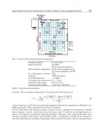
Fig. 3. A single slosh mass-spring model for a spacecraft with throttable side thrusters.
The control objective is to design feedback controllers so that the controlled spacecraft
accomplishes a given planar maneuver, that is a change in the translational velocity vector
and the attitude of the spacecraft, while attenuating the slosh mode. The work in (Cho et al.,
2000b) considers a constant thrust F

> 0 and develops a feedback law (using a backstepping
approach) to stabilize the system (7)-(10) to a relative equilibrium defined by a constant
acceleration in the axial direction. A slightly modified and relatively simpler feedback
controller that uses a Lyapunov approach (without resorting to backstepping) can be found
in (Reyhanoglu, 2003). In the subsequent development, we will develop feedback controllers
to achieve the same control objective using the system (11)-(14).
The mass-spring analogy is related to the pendulum analogy, in which the oscillation
frequency of the mass-spring element represents the lowest frequency sloshing mode (Sidi,
1997).
Consider a rigid spacecraft moving on a plane as indicated in Fig. 3, where v
x
, v
z
are the axial
and transverse components, respectively, of the velocity of the center of the fuel tank, and θ
denotes the attitude angle of the spacecraft with respect to a fixed reference. The slosh mode
is modeled by a point mass m
f
whose relative position along the body z-axis is denoted by s;a
restoring force
−ks acts on the mass whenever the mass is displaced from its neutral position
s
= 0. As in the previous model, a thrust F, which is assumed to act through the spacecraft
center of mass along the spacecraft’s longitudinal axis, a transverse force f , and a pitching
moment M are available for control purposes. The constants in the problem are the spacecraft
mass m and moment of inertia I,thefuelmassm
f
, and the distance b between the body z-axis
and the spacecraft center of mass location along the longitudinal axis. The parameters m
f

, k
and b depend on the shape of the fuel tank, the characteristics of the fuel and the fill ratio of
the fuel tank.
The position vector of the fuel mass m
f
in the spacecraft-fixed coordinate frame is given by
r
f
= x
ˆ
i +(z + s)
ˆ
k,
554
Advances in Spacecraft Technologies
Modeling and Control of Space Vehicles with Fuel Slosh Dynamics 7
and the inertial velocity of the fuel can be computed as
˙
r
f
=[
˙
x
+(z + s)
˙
θ
]
ˆ
i
+[

˙
z
− x
˙
θ +
˙
s
]
ˆ
k
=(v
x
+ s
˙
θ)
ˆ
i +(v
z
+
˙
s
)
ˆ
k. (15)
Thus, under the indicated assumptions, the Lagrangian can be found as
L
=
1
2
m

˙
r
2
+
1
2
m
f
˙
r
2
f
+
1
2
I
˙
θ
2
−
1
2
ks
2
=
1
2
m
[v
2

x
+(v
z
+ b
˙
θ)
2
]+
1
2
m
f
[(v
x
+ s
˙
θ)
2
+(v
z
+
˙
s
)
2
]+
1
2
I
˙

θ
2
−
1
2
ks
2
. (16)
Applying equations (1)-(3) with
η
= s, R =
1
2
c
˙
s
2
, v =
⎛
⎝
v
x
0
v
z
⎞
⎠
, ω
=
⎛

⎝
0
˙
θ
0
⎞
⎠
, τ
t
=
⎛
⎝
F
0
f
⎞
⎠
, τ
r
=
⎛
⎝
0
M
+ fb
0
⎞
⎠
,
the equations of motion can be obtained as

(m + m
f
)(
˙
v
x
+
˙
θv
z
)+m
f
s
¨
θ + mb
˙
θ
2
+ 2m
f
˙
s
˙
θ
= F , (17)
(m + m
f
)(
˙
v

z
−
˙
θv
x
)+mb
¨
θ + m
f
¨
s
− m
f
s
˙
θ
2
= f , (18)
(I + mb
2
+ m
f
s
2
)
¨
θ
+ m
f
s(

˙
v
x
+
˙
θv
z
)+2m
f
s
˙
s
˙
θ + mb(
˙
v
z
−
˙
θv
x
)=M + bf, (19)
m
f
(
¨
s
+
˙
v

z
−
˙
θv
x
− s
˙
θ
2
)+ks + c
˙
s = 0 . (20)
The control objective is again to design feedback controllers so that the controlled spacecraft
accomplishes a given planar maneuver, that is a change in the translational velocity vector
and the attitude of the spacecraft, while suppressing the slosh mode.
In this section, we restrict the development to the single slosh pendulum model of a spacecraft
with a gimballed thrust engine, i.e. we design feedback controllers for the system (11)-(14)
only. In particular, we study the problem of controlling the system to a relative equilibrium
defined by a constant acceleration in the axial direction.
To obtain the linearized equations of motion, assume small gimbal deflection so that cos δ ≈ 1
and sin δ
≈ δ, and we rewrite (11)-(14) as:
(m + m
f
)a
x
+ m
f
a(
¨

θ
+
¨
ψ
)sin ψ + mb
˙
θ
2
+ m
f
a(
˙
θ
+
˙
ψ
)
2
cosψ = F , (21)
(m + m
f
)a
z
+ m
f
a(
¨
θ
+
¨

ψ
)cos ψ + mb
¨
θ − m
f
a(
˙
θ
+
˙
ψ
)
2
sinψ = Fδ , (22)
(I + mb
2
)
¨
θ + mb a
z
− 
˙
ψ = M + Fl δ, (23)
(I
f
+ m
f
a
2
)(

¨
θ
+
¨
ψ
)+m
f
a(a
x
sinψ + a
z
cos ψ)+
˙
ψ = 0, (24)
where l
= b + p and (a
x
, a
z
)=(
˙
v
x
+
˙
θv
z
,
˙
v

z
−
˙
θv
x
) are the axial and transverse components
of the acceleration of the center of the fuel tank. The number of equations of motion can
555
Modeling and Control of Space Vehicles with Fuel Slosh Dynamics
8 Advances in Spacecraft Technologies
be reduced to two by solving equations (21) and (22) for a
x
and a
z
, and eliminating these
accelerations from equations (23) and (24).
[I + m
∗
(b
2
− abcos ψ )]
¨
θ
− m
∗
ab
¨
ψ cosψ + m
∗
ab(

˙
θ
+
˙
ψ
)
2
sinψ − 
˙
ψ = M + b
∗
Fδ , (25)
[I
f
+ m
∗
(a
2
− abcos ψ )]
¨
θ
+(I
f
+ m
∗
a
2
)
¨
ψ

+(a
∗
F − m
∗
ab
˙
θ
2
)sin ψ + 
˙
ψ = −a
∗
Fδ cosψ , (26)
where
m
∗
=
mm
f
m + m
f
, a
∗
=
m
f
a
m + m
f
, b

∗
=
m
f
b
m + m
f
+ d.
As mentioned previously, without loss of generality, we will assume that the desired
equilibrium is given by:
(θ
∗
,
˙
θ
∗
,ψ
∗
,
˙
ψ
∗
)=(0, 0,0,0).
Assuming that θ,
˙
θ, ψ,and
˙
ψ are small, the following linearized equations can be obtained:
I
1

¨
θ − I
2
¨
ψ
− 
˙
ψ = M + b
∗
Fδ , (27)
I
3
¨
θ
+ I
4
¨
ψ
+ a
∗
Fψ + 
˙
ψ = −a
∗
Fδ . (28)
where
I
1
= I + m
∗

(b
2
− ab) , I
2
= m
∗
ab,
I
3
= I
f
+ m
∗
(a
2
− ab) , I
4
= I
f
+ m
∗
a
2
.
For the linearized system (27)-(28), the state variables are the attitude angle θ, the slosh angle
ψ, and their time derivatives. The collection of these state variables is defined as the partial
state vector given by
x
=[θ,
˙

θ, ψ,
˙
ψ]
T
.
Let u
=[δ, M]
T
denote the control input vector. Then, the state space equations can be written
as:
˙x
= Ax + Bu , (29)
where
A
=
⎡
⎢
⎢
⎢
⎢
⎣
01 0 0
00
−
a
∗
I
2
F
Δ

−
(
I
2
− I
4
)
Δ
00 0 1
00
−
a
∗
I
1
F
Δ
−
(
I
1
+ I
3
)
Δ
⎤
⎥
⎥
⎥
⎥

⎦
, B
=
⎡
⎢
⎢
⎢
⎢
⎣
00
−
(
I
2
a
∗
− I
4
b
∗
)F
Δ
I
4
Δ
00
−
(
I
1

a
∗
+ I
3
b
∗
)F
Δ
−
I
3
Δ
⎤
⎥
⎥
⎥
⎥
⎦
. (30)
and
Δ
= I
1
I
4
+ I
2
I
3
.

We consider an LQR (Linear Quadratic Regulator) controller of the form
u
= −Kx (31)
that minimizes the quadratic cost function
J
=

∞
0
(x
T
Qx + u
T
Ru)dt , (32)
556
Advances in Spacecraft Technologies
Modeling and Control of Space Vehicles with Fuel Slosh Dynamics 9
where Q is a symmetric positive-semidefinite weighting matrix and R is a positive-definite
weighting matrix.
The optimal control gain matrix K is found by solving the corresponding matrix Riccati
equation (or using MATLAB’s lqr function). This controller is then applied to the actual
nonlinear system (11)-(14). The simulation results show that the linear controller (31) results
in undesirable steady-state errors in transverse velocity (see Figure 4).
Consider the single slosh pendulum model of a spacecraft with a gimballed thrust engine
shown in Fig. 2. If the thrust F is a positive constant, and if the gimbal deflection angle and
pitching moment are zero, δ
= M = 0, then the spacecraft and fuel slosh dynamics have a
relative equilibrium defined by
v
∗

x
(t)=
F
m + m
f
t + v
x0
, v
z
= v
∗
z
,
θ
= θ
∗
,
˙
θ = 0,ψ = 0,
˙
ψ = 0,
where v
∗
z
and θ
∗
are arbitrary constants, and v
x0
is the initial axial velocity of the spacecraft.
Note that θ

∗
and v
∗
z
are the desired attitude angle and transverse velocity, chosen as zero
here. Now assume the axial acceleration term a
x
is not significantly affected by small
gimbal deflections, pitch changes and fuel motion (an assumption verified in simulations).
Consequently, equation (11) becomes:
˙
v
x
+
˙
θv
z
=
F
m + m
f
. (33)
Substituting this approximation leads to the following equations of motion for the transverse,
pitch and slosh dynamics:
(m + m
f
)(
˙
v
z

−
˙
θv
x
(t)) + m
f
a(
¨
θ +
¨
ψ
)cos ψ + mb
¨
θ − m
f
a(
˙
θ +
˙
ψ
)
2
sinψ = Fδ , (34)
(I + mb
2
)
¨
θ
+ mb(
˙

v
z
−
˙
θv
x
(t)) − 
˙
ψ = M + Fl δ, (35)
(I
f
+ m
f
a
2
)(
¨
θ
+
¨
ψ
)+m
f
a
F
m + m
f
sinψ + m
f
a(

˙
v
z
−
˙
θv
x
(t))cos ψ + 
˙
ψ = 0, (36)
where v
x
(t) is considered as an exogenous input.
Define the error variable
˜
v
x
= v
x
(t) − v
∗
x
(t) .
Then, the equations of motion can be written in the following form
˙
˜
v
x
= −
˙

θv
z
, (37)
˙
v
z
= u
1
+
˙
θ
(
˜
v
x
+ v
∗
x
(t)), (38)
¨
θ
= u
2
, (39)
¨
ψ
= −u
1
ccos ψ − u
2

− dsin ψ − e
˙
ψ, (40)
where
c
=
m
f
a
I
f
+ m
f
a
2
, d =
Fc
m + m
f
, e =

I
f
+ m
f
a
2
,
557
Modeling and Control of Space Vehicles with Fuel Slosh Dynamics

10 Advances in Spacecraft Technologies
and (u
1
, u
2
) are new control inputs defined as

u
1
u
2

= M
−1
(ψ)

F sinδ
− m
f
a
¨
ψ cosψ + m
f
a(
˙
θ
+
˙
ψ
)

2
sinψ
M
+ Flsinδ + 
˙
ψ

, (41)
where
M
(ψ)=

m
f
acos ψ + mb m + m
f
I + mb
2
mb

. (42)
Now, we consider the following candidate Lyapunov function for the system (37)-(40):
V
=
r
1
2
(
˜
v

2
x
+ v
2
z
)+
r
2
2
θ
2
+
r
3
2
˙
θ
2
+ r
4
d(1 − cosψ)+
r
4
2
(
˙
θ
+
˙
ψ

)
2
, (43)
where r
1
, r
2
, r
3
,andr
4
are positive constants. The function V is positive definite in the domain
D
= {(
˜
v
x
, v
z
, θ,
˙
θ, ψ,
˙
ψ) |−π < ψ < π}.
ThetimederivativeofV along the trajectories of (37)-(40) is
˙
V =[r
1
v
z

− r
4
c(
˙
θ +
˙
ψ
)cos ψ] u
1
+[r
1
v
∗
x
(t)v
z
+ r
2
θ + r
3
u
2
+ r
4
e(
˙
θ +
˙
ψ
) − r

4
dsin ψ]
˙
θ
− r
4
e(
˙
θ +
˙
ψ
)
2
.
(44)
Clearly, the feedback laws
u
1
= −l
1
[r
1
v
z
− r
4
c(
˙
θ +
˙

ψ
)cos ψ], (45)
u
2
= −l
2
˙
θ
− [
r
1
r
3
v
∗
x
(t)v
z
+
r
2
r
3
θ] −
r
4
r
3
[e(
˙

θ
+
˙
ψ
) − dsin ψ)], (46)
where l
1
and l
2
are positive constants, yield
˙
V
= −l
1
[r
1
v
z
− r
4
c(
˙
θ +
˙
ψ
)cos ψ]
2
− l
2
˙

θ
2
− r
4
e(
˙
θ +
˙
ψ
)
2
,
which satisfies
˙
V
≤ 0inD. Using LaSalle’s principle, it is easy to prove asymptotic stability of
the origin of the closed loop defined by the equations (37)-(40) and the feedback control laws
(45)-(46). Note that the positive gains r
i
, i = 1, 2, 3, 4 and l
j
, j = 1, 2, can be chosen arbitrarily
to achieve good closed loop responses.
The feedback control laws developed in the previous sections are implemented here for a
spacecraft. The physical parameters used in the simulations are m
= 600 kg, I = 720kg/m
2
,
m
f

= 100 kg, I
f
= 90 kg/m
2
, a = 0.2 m, b = 0.3 m, p = 0.2 m, F = 2300 N and  = 0.19 kg · m
2
/s.
We consider stabilization of the spacecraft in orbital transfer, suppressing the transverse and
pitching motion of the spacecraft and sloshing of fuel while the spacecraft is accelerating. In
other words, the control objective is to stabilize the relative equilibrium corresponding to a
constant axial spacecraft acceleration of 3.286 m/s
2
and v
z
= θ =
˙
θ = ψ =
˙
ψ
= 0.
558
Advances in Spacecraft Technologies
Modeling and Control of Space Vehicles with Fuel Slosh Dynamics 11
In this section, an LQR controller of the form (31) is applied to the complete nonlinear system
(11)-(14). Using the physical parameters given above, the A and B matrices defined by
equation (30) were computed as
A
=
⎡
⎢

⎢
⎣
01 0 0
00
−0.005 0.0002
00 0 1
00
−0.6987 −0.0023
⎤
⎥
⎥
⎦
,
B
=
⎡
⎢
⎢
⎣
00
0.7629 0.0014
00
−1.4243 −0.0013
⎤
⎥
⎥
⎦
.
Choosing the weighting matrices as
Q

=
⎡
⎢
⎢
⎣
1000
0100
0010
0001
⎤
⎥
⎥
⎦
,
R
=

10 0
00.01

,
the LQR gain matrix for the linear system (29) was found as
K
=

0.3153 1.2214
−0.3496 −0.2696
0.7627 2.8027 0.6462 0.0764

.

This gain matrix yields the following eigenvalues for the closed-loop system matrix A
− BK:
(−0.3312 ± 0.8233 i, −0.3297 ± 0.3294i).
Time responses shown in Fig. 4 and Fig. 5 correspond to the initial conditions v
x0
= 10000 m/s,
v
z0
= 0, θ
0
= 2
o
,
˙
θ
0
= 0.57
o
/s, ψ
0
= 15
o
,and
˙
ψ
0
= 0. As can be seen in the figures, the LQR
controller stabilizes the pitch and slosh dynamics, but fails to stabilize the transverse velocity
to zero. The controller results in a steady-state error of v
z

= −349.1 m/s.
In this section, we demonstrate the effectiveness of the Lyapunov-based controller (45)-(46) by
applying to the complete nonlinear system (11)-(14).
Time responses shown in Fig. 6 and Fig. 7 correspond to the initial conditions v
x0
= 10000 m/s,
v
z0
= 350 m/s, θ
0
= 2
o
,
˙
θ
0
= 0.57
o
/s, ψ
0
= 30
o
,and
˙
ψ
0
= 0. As can be seen in the figures, the
transverse velocity, attitude angle and the slosh angle converge to the relative equilibrium at
zero while the axial velocity v
x

increases and
˙
v
x
tends asymptotically to 3.286m/s
2
.Notethat
there is a trade-off between good responses for the directly actuated degrees of freedom (the
transverse and pitch dynamics) and good responses for the unactuated degree of freedom
(the slosh dynamics); the controller given by (45)-(46) with parameters r
1
= 10
−7
, r
2
= 10, r
3
=
10
2
, r
4
= 10
−2
, l
1
= 10
3
, l
2

= 1 represents one example of this balance.
559
Modeling and Control of Space Vehicles with Fuel Slosh Dynamics
12 Advances in Spacecraft Technologies
0 5 10 15 20 25 30
0.99
1
1.01
x 10
4
v
x
(m/s)
0 5 10 15 20 25 30
−1000
0
1000
v
z
(m/s)
0 5 10 15 20 25 30
−5
0
5
θ (deg)
0 5 10 15 20 25 30
−20
0
20
ψ (deg)

Time (s)
Fig. 4. Time responses of state variables v
x
, v
z
, θ,andψ (LQR controller).
0 5 10 15 20 25 30
−4
−2
0
2
4
δ (deg)
0 5 10 15 20 25 30
−0.05
0
0.05
0.1
0.15
M (N.m)
Time (s)
Fig. 5. Gimbal deflection angle δ and pitching moment M (LQR controller).
0 5 10 15 20 25 30
0.98
1
1.02
x 10
4
v
x

(m/s)
0 5 10 15 20 25 30
−500
0
500
v
z
(m/s)
0 5 10 15 20 25 30
0
2
4
θ (deg)
0 5 10 15 20 25 30
−50
0
50
ψ (deg)
Time (s)
Fig. 6. Time responses of state variables v
x
, v
z
, θ,andψ (Lyapunov-based controller).
560
Advances in Spacecraft Technologies
Modeling and Control of Space Vehicles with Fuel Slosh Dynamics 13
0 5 10 15 20 25 30
−15
−10

−5
0
5
δ (deg)
0 5 10 15 20 25 30
−50
0
50
100
150
M (N.m)
Time (s)
Fig. 7. Gimbal deflection angle δ and pitching moment M (Lyapunov-based controller).
We have shown that a linear controller, while successful in stabilizing the pitch and slosh
dynamics, fails to control the transverse dynamics of a spacecraft. We have designed a
Lyapunov-based nonlinear feedback control law that achieves stabilization of the pitch and
transverse dynamics as well as suppression of the slosh mode, while the spacecraft accelerates
in the axial direction. The effectiveness of this control feedback law has been illustrated
through a simulation example.
The many avenues considered for future research include problems involving
higher-frequency slosh modes, multiple propellant tanks, and three dimensional maneuvers.
Future research also includes designing nonlinear control laws that achieve robustness,
insensitivity to system and control parameters, and improved disturbance rejection. In
particular, we plan to explore the use of sliding mode controllers to accomplish this.
Adler, J. M., Lee, M. S. & Saugen, J. D. (1991). Adaptive control of propellant slosh for launch
vehicles, SPIE Sensors and Sensor Integration 1480: 11–22.
Biswal, K. C., Bhattacharyya, S. K. & Sinha, P. K. (2004). Dynamic characteristics of liquid
filled rectangular tank with baffles, IE (I) Journal-CV 84: 145–148.
Blackburn, T. R. & Vaughan, D. R. (1971). Application of linear optimal control and
filtering theory to the saturn v launch vehicle, IEEE Transactions on Automatic Control

16(6): 799–806.
Bryson, A. E. (1994). ControlofSpacecraftandAircraft, Princeton University Press.
Cho, S., McClamroch, N. H. & Reyhanoglu, M. (2000a). Dynamics of multibody vehicles
and their formulation as nonlinear control systems, Proceedings of American Control
Conference, pp. 3908–3912.
Cho, S., McClamroch, N. H. & Reyhanoglu, M. (2000b). Feedback control of a space vehicle
with unactuated fuel slosh dynamics, Proceedings of AIAA Guidance, Navigation, and
Control Conference, pp. 354–359.
Feddema, J. T., Dohrmann, C. R., Parker, G. G., Robinett, R. D., Romero, V. J. & Schmitt,
D. J. (1997). Control for slosh-free motion of an open container, IEEE Control Systems
561
Modeling and Control of Space Vehicles with Fuel Slosh Dynamics
14 Advances in Spacecraft Technologies
Magazine pp. 29–36.
Freudenberg, J. & Morton, B. (1992). Robust control of a booster vehicle using h
∞
and
ssv techniques, Proceedings of the 31st IEEE Conference on Decision and Control,
pp. 2448–2453.
Grundelius, M. (2000). Iterative optimal control of liquid slosh in an industrial packaging
machine, Proceedings of the 39th IEEE Conference on Decision and Control, pp. 3427–3432.
Grundelius, M. & Bernhardsson, B. (1999). Control of liquid slosh in an industrial packaging
machine, Proceedings of IEEE International Conference on Control Applications,
pp. 1654–1659.
Hubert, C. (2003). Behavior of Spinning Space Vehicles with Onboard Liquids, NASA/KSC
Contract NAS10-02016.
Hubert, C. (2004). Design and flight performance of a system for rapid attitude maneuvers by
a spinning vehicle, Proceedings of the 27th Annual AAS Guidance and Control Conference.
Meirovitch, L. & Kwak, M. K. (1989). State equations for a spacecraft with maneuvering
flexible appendages in terms of quasi-coordinates, Applied Mechanics Reviews

42(11): 161–170.
Peterson, L. D., Crawley, E. F. & Hansman, R. J. (1989). Nonlinear fluid slosh coupled to the
dynamics of a spacecraft, AIAA Journal 27(9): 1230–1240.
Reyhanoglu, M. (2003). Maneuvering control problems for a spacecraft with unactuated fuel
slosh dynamics, Proceedings of IEEE Conference on Control Applications, pp. 695–699.
Reyhanoglu, M., Cho, S. & McClamroch, N. H. (2000). Discontinuous feedback control of a
special class of underactuated mechanical systems, International Journal of Robust and
Nonlinear Control 10(4): 265–281.
Reyhanoglu, M., van der Schaft, A. J., McClamroch, N. & Kolmanovsky, I. (1996). Nonlinear
control of a class of underactuated systems, Proceedings of IEEE Conference on Decision
and Control, pp. 1682–1687.
Reyhanoglu, M., van der Schaft, A. J., McClamroch, N. & Kolmanovsky, I. (1999). Dynamics
and control of a class of underactuated mechanical systems, IEEE Transactions on
Automatic Control 44(9): 1663–1671.
Sidi, M. J. (1997). Spacecraft Dynamics and Control, Cambridge University Press, New York.
Terashima, K. & Schmidt, G. (1994). Motion control of a cart-based container considering
suppression of liquid oscillations, Proceedings of IEEE International Symposium on
Industrial Electronics, pp. 275–280.
Venugopal, R. & Bernstein, D. S. (1996). State space modeling and active control of slosh,
Proceedings of IEEE International Conference on Control Applications, pp. 1072–1077.
Wie, B. (2008). Space Vehicle Dynamics and Control, AIAA Education Series.
Yano, K., Higashikawa, S. & Terashima, K. (2001). Liquid container transfer control on 3d
transfer path by hybrid shaped approach, Proceedings of IEEE International Conference
on Control Applications, pp. 1168–1173.
Yano, K. & Terashima, K. (2001). Robust liquid container transfer control for complete sloshing
suppression, IEEE Transactions on Control Systems Technology 9(3): 483–493.
Yano, K., Toda, T. & Terashima, K. (2001). Sloshing suppression control of automatic pouring
robot by hybrid shape approach, Proceedings of the 40th IEEE Conference on Decision
and Control, pp. 1328–1333.
562

Advances in Spacecraft Technologies
0
Synchronization of Target Tracking Cascaded
Leader-Follower Spacecraft Formation
Rune Schlanbusch and Per Johan Nicklasson
Department of Technology, Narvik University College, PB 385, AN-8505 Narvik
Norway
1. Introduction
In recent years, formation flying has become an increasingly popular subject of study. This
is a new method of performing space operations, by replacing large and complex spacecraft
with an array of simpler micro-spacecraft bringing out new possibilities and opportunities
of cost reduction, redundancy and improved resolution aspects of onboard payload. One
of the main challenges is the requirement of synchronization between spacecraft; robust
and reliable control of relative position and attitude are necessary to make the spacecraft
cooperate to gain the possible advantages made feasible by spacecraft formations. For
fully autonomous spacecraft formations both path- and attitude-planning must be performed
on-line which introduces challenges like collision avoidance and restrictions on pointing
instruments towards required targets, with the lowest possible fuel expenditure. The system
model is a key element to achieve a reliable and robust controller.
1.1 Previous work
The simplest Cartesian model of relative motion between two spacecraft is linear and known
as the Hill (Hill, 1878) or Clohessy-Wiltshire (Clohessy & Wiltshire, 1960) equations; a
linear model based on assumptions of circular orbits, no orbital perturbations and small
relative distance between spacecraft compared with the distance from the formation to
the center of the Earth. As the visions for tighter spacecraft formations in highly elliptic
orbits appeared, the need for more detailed models arose, especially regarding orbital
perturbations. This resulted in nonlinear models as presented in e.g. (McInnes, 1995; Wang
& Hadaegh, 1996), and later in (Yan et al., 2000a) and (Kristiansen, 2008), derived for
arbitrary orbital eccentricity and with added terms for orbital perturbations. Most previous
work on reference generation are concerned with translational trajectory generation for fuel

optimal reconfiguration and formation keeping such as in (Wong & Kapila, 2005) where
a formation located at the Sun-Earth L
2
Langrange Point is considered, while (Yan et al.,
2009) proposed two approaches to design perturbed satellite formation relative motion orbits
using least-square techniques. Trajectory optimization for satellite reconfiguration maneuvers
coupled with attitude constraints have been investigated in (Garcia & How, 2005) where
a path planner based on rapidly-exploring random tree is used in addition to a smoother
function. Coupling between the position and attitude is introduced by the pointing constrains,
and thus the trajectory design must be solved as a single 6N Degrees of Freedom (DOF)
problem instead of N separate 6 DOF problems.
25
2 Advances in Spacecraft Technologies
Ground target tracking for spacecraft has been addressed by several other researchers, such
as (Goerre & Shucker, 1999; Chen et al., 2000; Tsiotras et al., 2001) and (Steyn, 2006) where
only one spacecraft is considered. The usual way to generate target tracking reference is
to find a vector pointing from the spacecraft towards a point on the planet surface where
the instrument is supposed to be pointing, and then the desired quaternions and angular
velocities are generated to ensure high accuracy tracking of the specified target point.
Due to the parameterization of the attitude for both Euler angles and the unit quaternion we
obtain a set of two equilibria of the closed-loop system of a rigid body, and possibilities of the
unwinding phenomenon. One approach to solve the problem of multiple equilibria is the use
of hybrid control (cf. (Liberzon, 2003), (Goebel et al., 2009)), and different solutions have been
presented, as in (Casagrande, 2008) for an underactuated non-symmetric rigid body, and by
(Mayhew et al., 2009) using quaternion-based hybrid feedback where the choice of rotational
direction is performed by a switching control law.
The nonlinear nature of the tracking control problem has been a challenging task in robotics
and control research. The so called passivity-based approach to robot control have gained much
attention, which, contrary to computed torque control, coupe with the robot control problem
by exploiting the robots’ physical structure (Berghuis & Nijmeijer, 1993). A simple solution to

the closed-loop passivity approach was proposed by (Takegaki & Arimoto, 1981) on the robot
position control problem. The natural extension the motion control task was solved in (Paden
& Panja, 1988), where the controller was called PD+, and in (Slotine & Li, 1987) where the
controller was called passivity- based sliding surface. The control structure was later applied for
spacecraft formation control in (Kristiansen, 2008).
For large systems, e.g. complex dynamical systems such as spacecraft formations, the
expression divide and conquer may seem appealing, and for good reasons; by dividing a
system into smaller parts, the difficulties of stability analysis and control design can be greatly
reduced. A particular case of such systems is cascaded structure which consists of a driving
system which is an input to the driven system through an interconnection (see (Lor
´
ıa & Panteley,
2005) and references therein).
The topic of cascaded systems have received a great deal of attention and has successfully
been applied to a wide number of applications. In (Fossen & Fjellstad, 1993) a cascaded
adaptive control scheme for marine vehicles including actuator dynamics was introduced,
while (Lor
´
ıa et al., 1998) solved the problem of synchronization of two pendula through use
of cascades. The authors of (Jankovi
´
c et al., 1996) studied the problem of global stabilisability
of feedforward systems by a systematic recursive design procedure for autonomous systems,
while time-varying systems were considered in (Jiang & Mareels, 1997) for stabilization of
robust control, while (Panteley & Lor
´
ıa, 1998) established sufficient conditions for Uniform
Global Asymptotical Stability (UGAS) for cascaded nonlinear time-varying systems. The
aspects of practical and semi-global stability for nonlinear time-varying systems in cascade
were pursued in (Chaillet, 2006) and (Chaillet & Lor

´
ıa, 2008). A stability analysis of spacecraft
formations including both leader and follower using relative coordinates was presented in
(Grøtli, 2010), where the controller-observer scheme was proven input-to-state-stable.
1.2 Contribution
In this paper we present a solution for real-time generation of attitude references
for a leader-follower spacecraft formation with target tracking leader and followers
complementing the measurement by pointing their instruments at a common target on the
Earth surface. The solution is based on a 6DOF model where each follower generates the
564
Advances in Spacecraft Technologies
Synchronization of Target Tracking Cascaded Leader-Follower Spacecraft Formation 3
attitude references in real-time based on relative translational motion between the leader
and its followers, which also ensures that the spacecraft are pointing at the target during
formation reconfiguration. We are utilizing a passivity-based sliding surface controller for
relative position and Uniform Global Practical Asymptotic Stability (UGPAS) is proven for
the equilibrium point of the closed-loop system. The control law is also adapted for hybrid
switching control with hysteresis for attitude tracking spacecraft in formation to ensure
robust stability when measurement noise is considered, and avoid unwinding, thus achieving
Uniform Practical Asymptotical Stability (UPAS) in the large on the set
S
3
× R
3
for the
equilibrium point of the closed-loop system. Simulation results are presented to show how
the attitude references are generated during a formation reconfiguration using the derived
control laws.
The rest of the paper is organized as follows. In Section 2we describe the modeling of relative
translation and rotation for spacecraft formations; in Section 3 we present a scheme were

the attitude reference for the leader and follower spacecraft is generated based on relative
coordinates; in Section 4 we present continuous control of relative translation and hybrid
control of relative rotation where stability of the overall system is proved through use of
cascades; in Section 5 we present simulation results and we conclude with some remarks in
Section 6.
2. Modeling
In the following, we denote by
˙
x the time derivative of a vector x, i.e.
˙
x = dx/dt, and moreover,
¨
x
= d
2
x/dt
2
. We denote by · the Euclidian norm of a vector and the induced L
2
norm of a
matrix. The cross-product operator is denoted S
(·), such that S(x)y = x ×y. Reference frames
are denoted by
F
(·)
, and in particular, the standard Earth-Centered Inertial (ECI) frame is
denoted
F
i
and The Earth-Centered Earth-Fixed (ECEF) frame is denoted F

e
. We denote by
ω
ω
ω
c
b,a
the angular velocity of frame F
a
relative to frame F
b
, referenced in frame F
c
. Matrices
representing rotation or coordinate transformation from frame
F
a
to frame F
b
are denoted
R
b
a
. When the context is sufficiently explicit, we may omit to write arguments of a function,
vector or matrix.
2.1 Cartesian coordinate frames
Basically there are two different approaches for modeling spacecraft formations: Cartesian
coordinates and orbital elements, which both have their pros and cons. The orbital element
method is often used to design formations concerning low fuel expenditure because of the
relationship towards natural orbits, while Cartesian models often are used where an orbit

with fixed dimensions are studied, which is the case in this paper.
The coordinate reference frames used throughout the paper are shown in Figure 1, and defined
as follows:
Leader orbit reference frame: The leader orbit frame, denoted
F
l
, has its origin located in
the center of mass of the leader spacecraft. The e
r
axis in the frame coincide with the vector
r
l
∈ R
3
from the center of the Earth to the spacecraft, and the e
h
axis is parallel to the orbital
angular momentum vector, pointing in the orbit normal direction. The e
θ
axis completes the
right-handed orthonormal frame. The basis vectors of the frame can be defined as
e
r
:=
r
l
r
l

, e

θ
:= S(e
h
)e
r
and e
h
:=
h
h
, (1)
where h
= S(r
l
)
˙
r
l
is the angular momentum vector of the orbit.
565
Synchronization of Target Tracking Cascaded Leader-Follower Spacecraft Formation
4 Advances in Spacecraft Technologies
Follower orbit reference frame: The follower orbit frame has its origin in the center of mass
of the follower spacecraft, and is denoted
F
f
. The vector pointing from the center of the Earth
to the frame origin is denoted r
f
∈ R

3
, and the frame is specified by a relative orbit position
vector p
=
[
x, y, z
]

expressed in F
l
components, and its unit vectors align with the basis
vectors of
F
l
. Accordingly,
p
= R
l
i
(r
f
−r
l
)=xe
r
+ ye
θ
+ ze
h
⇒ r

f
= R
i
l
p + r
l
. (2)
2.2 Quaternions and kinematics
The attitude of a rigid body is often represented by a rotation matrix R ∈ SO(3) fulfilling
SO
(3)={R ∈ R
3×3
: R

R = I, detR = 1} , (3)
which is the special orthogonal group of order three, where I denotes the identity matrix.
A rotation matrix for a rotation θ about an arbitrary unit vector k
k
k
∈ R
3
can be angle-axis
parameterized as –cf. (Egeland & Gravdahl, 2002),
R
k,θ
= I + S(k)sinθ + S
2
(k)(1 −cosθ) , (4)
and coordinate transformation of a vector r from frame a to frame b is written as r
b

= R
b
a
r
a
.
The rotation matrix in (4) can be expressed by an Euler parameter representation as
R
= I + 2ηS(

)+2S
2
(

) , (5)
where the matrix S
(·) is the cross product operator
S
(

)=

× =
⎡
⎣
0 −
z

y


z
0 −
x
−
y

x
0
⎤
⎦
, 


=
⎡
⎣

x

y

z
⎤
⎦
. (6)
Quaternions are often used to parameterize members of SO
(3) where the unit quaternion is
defined as q
=[η, 




]

∈S
3
= {x ∈ R
4
: x

x = 1}, where η = cos(θ/2) ∈ R is the scalar
Leader
Follower
r
l
r
f
i
x
i
y
i
z
e
r
e
θ
e
h
p

Fig. 1. Reference coordinate frames.
566
Advances in Spacecraft Technologies
Synchronization of Target Tracking Cascaded Leader-Follower Spacecraft Formation 5
part and 

 = k sin(θ/2) ∈ R
3
is the vector part. The set S
3
forms a group with quaternion
multiplication, which is distributive and associative, but not commutative, and the quaternion
product is defined as
q
1
⊗q
2
=

η
1
η
2
−



1




2
η
1



2
+ η
2



1
+ S(


1
)


2

. (7)
The inverse rotation can be performed by using the inverse conjugate of q given by
¯
q
=
[
η, −




]

. The time derivative of the rotation matrix is
˙
R
a
b
= S

ω
ω
ω
a
a,b

R
a
b
= R
a
b
S

ω
ω
ω
b

a,b

, (8)
and the kinematic differential equations may be expressed as
˙
q
= T(q)ω
ω
ω, T(q)=
1
2

−


T
ηI + S(

)

∈ R
4×3
. (9)
2.2.1 Relative translation
The fundamental differential equation of the two-body problem can be expressed as (cf.
(Battin, 1999))
¨
r
s
= −

μ
r
3
s
r
s
+
f
sd
m
s
+
f
sa
m
s
, (10)
where f
sd
∈ R
3
is the perturbation term due to external effects, f
sa
∈ R
3
is the actuator force,
m
s
is the mass of the spacecraft, and super-/sub-script s denotes the spacecraft in question, so
s

= l, f for the leader and follower spacecraft respectively. The spacecraft masses are assumed
to be small relative to the mass of the Earth M
e
,soμ ≈ GM
e
, where G is the gravitational
constant. According to (2) the relative position between the leader and follower spacecraft
may be expressed as
R
i
l
p = r
f
−r
l
, (11)
and by differentiating twice we obtain
R
i
l
¨
p
+ 2R
i
l
S(ω
ω
ω
l
i,l

)
˙
p
+ R
i
l

S
2
(ω
ω
ω
l
i,l
)+S(
˙
ω
ω
ω
l
i,l
)

p
=
¨
r
f
−
¨

r
l
. (12)
By inserting (10), the right hand side of (12) may be written as
¨
r
f
−
¨
r
l
= −
μ
r
3
f
r
f
+
f
fd
m
f
+
f
fa
m
f
+
μ

r
3
l
r
l
−
f
ld
m
l
−
f
la
m
l
, (13)
and by inserting (2) into (13), we find that
m
f
(
¨
r
f
−
¨
r
l
)=−m
f
μ


1
r
3
f
−
1
r
3
l

r
l
+
R
i
l
p
r
3
f

+ f
fa
+ f
fd
−
m
f
m

l
(f
la
+ f
ld
) . (14)
Moreover, by inserting (14) into (12), and rearranging the terms we obtain
m
f
¨
p
+ C
t
(ω
ω
ω
l
i,l
)
˙
p
+ D
t
(
˙
ω
ω
ω
l
i,l

,ω
ω
ω
l
i,l
,r
f
)p + n
t
(r
l
,r
f
)=F
a
+ F
d
, (15)
567
Synchronization of Target Tracking Cascaded Leader-Follower Spacecraft Formation
6 Advances in Spacecraft Technologies
where
C
t
(ω
ω
ω
l
i,l
)=2m

f
S(ω
ω
ω
l
i,l
) (16)
is a skew-symmetric matrix,
D
t
(
˙
ω
ω
ω
l
i,l
,ω
ω
ω
l
i,l
,r
f
)=m
f

S
2
(ω

ω
ω
l
i,l
)+S(
˙
ω
ω
ω
l
i,l
)+
μ
r
3
f
I

(17)
may be viewed as a time-varying potential force, and
n
t
(r
l
,r
f
)=μm
f
R
l

i

1
r
3
f
−
1
r
3
l

r
l
(18)
is a nonlinear term. The composite perturbation force F
d
and the composite relative control
force F
a
are respectively written as
F
d
= R
l
i

f
fd
−

m
f
m
l
f
ld

and F
a
= R
l
i

f
fa
−
m
f
m
l
f
la

. (19)
Note that all forces f are presented in the inertial frame. If the forces are computed in another
frame, the rotation matrix should be replaced accordingly. The orbital angular velocity and
angular acceleration can be expressed as ω
ω
ω
i

i,l
= S(r
l
)v
l
/r

l
r
l
, and
˙
ω
ω
ω
i
i,l
=
r

l
r
l
S(r
l
)a
l
−2v

l

r
l
S(r

l
)v
l
(r

l
r
l
)
2
, (20)
respectively.
2.2.2 Relative rotation
With the assumptions of rigid body movement, the dynamical model of a spacecraft can be
found from Euler’s momentum equations as (Sidi, 1997)
J
s
˙
ω
ω
ω
sb
i,sb
= −S(ω
ω
ω

sb
i,sb
)J
s
ω
ω
ω
sb
i,sb
+ τ
τ
τ
sb
sd
+ τ
τ
τ
sb
sa
(21)
ω
ω
ω
sb
s,sb
= ω
ω
ω
sb
i,sb

−R
sb
i
ω
ω
ω
i
i,s
, (22)
where J
s
= diag{J
sx
, J
sy
, J
sz
}∈R
3×3
is the spacecraft moment of inertia matrix, τ
τ
τ
sb
sd
∈ R
3
is
the total disturbance torque, τ
τ
τ

sb
sa
∈ R
3
is the total actuator torque and ω
ω
ω
i
i,s
= S(r
s
)v
s
/r

s
r
s
is
the orbital angular velocity. Rotation from the leader body frame to the inertial frame are
denoted q
i
lb
, while rotation from the follower body frame to the inertial frame are denoted
q
i
fb
. Relative rotation between the follower and leader body frame is found by applying the
quaternion product (cf. (7)) expressed as
q

lb
fb
= q
i
fb
⊗
¯
q
i
lb
, (23)
and with a slightly abuse of notation we denote q
l
= q
i
lb
and q
f
= q
lb
fb
. The relative attitude
dynamics may be expressed as (cf. (Yan et al., 2000b; Kristiansen, 2008))
J
f
˙
ω
ω
ω
+ J

f
S(R
fb
lb
ω
ω
ω
lb
i,lb
)ω
ω
ω −J
f
R
fb
lb
J
−1
l
S(ω
ω
ω
lb
i,lb
)J
l
ω
ω
ω
lb

i,lb
(24)
+ S(ω
ω
ω + R
fb
lb
ω
ω
ω
lb
i,lb
)J
f
(ω
ω
ω + R
fb
lb
ω
ω
ω
lb
i,lb
)=Υ
d
+ Υ
a
,
568

Advances in Spacecraft Technologies
Synchronization of Target Tracking Cascaded Leader-Follower Spacecraft Formation 7
where
ω
ω
ω
= ω
ω
ω
fb
i, fb
−R
fb
lb
ω
ω
ω
lb
i,lb
(25)
is the relative angular velocity between the follower body reference frame and the leader body
reference frame expressed in the follower body reference frame,
Υ
d
= τ
τ
τ
fb
fd
−J

f
R
fb
lb
J
−1
l
τ
τ
τ
lb
ld
, Υ
a
= τ
τ
τ
fb
fa
−J
f
R
fb
lb
J
−1
l
τ
τ
τ

lb
la
(26)
are the relative perturbation torque and actuator torque, respectively. For simplicity (24) may
be rewritten as
J
f
˙
ω
ω
ω
+ C
r
(ω
ω
ω)ω
ω
ω + n
r
(ω
ω
ω)=Υ
d
+ Υ
a
, (27)
where
C
r
(ω

ω
ω)=J
f
S(R
fb
lb
ω
ω
ω
lb
i,lb
)+S(R
fb
lb
ω
ω
ω
lb
i,lb
)J
f
−S(J
f
(ω
ω
ω + R
fb
lb
ω
ω

ω
lb
i,lb
)) (28)
is a skew-symmetric matrix, and
n
r
(ω
ω
ω)=S(R
fb
lb
ω
ω
ω
lb
i,lb
)J
f
R
fb
lb
ω
ω
ω
lb
i,lb
−J
f
R

fb
lb
J
−1
l
S(ω
ω
ω
lb
i,lb
)J
l
ω
ω
ω
lb
i,lb
(29)
is a nonlinear term.
3. Reference generation
Our objective for the spacecraft formation is to have each spacecraft, including the leader,
tracking a fixed point located at the surface of e.g. the Earth by specifying a tracking direction
of the selected pointing axis where a measurement instrument is mounted such as e.g. a
camera or antenna. The target is chosen by the spacecraft operator as a given set of coordinates
such as latitude
(φ) and longitude (λ). The vector pointing from the center of Earth to the
target in an Earth Centered Earth Fixed (ECEF) frame is obtained by applying
r
e
t

=
⎡
⎣
cos
(φ) cos(λ)
cos(φ) sin(λ)
sin(φ)
⎤
⎦
r
e
(30)
where r
e
= 6378.137 × 10
3
m is the Earth radii. It is assumed a perfect spherical Earth;
alternatively a function of the Earth radii may be used as r
e
(λ,φ) with longitude and latitude
as arguments. If we assume that the Earth has a constant angular rate ω
e
= 7.292115 ×
10
−5
rad/s around its rotation axis we can rotate the target vector to ECI coordinates by
utilizing
r
t
= R

i
e
r
e
t
(31)
where the rotation matrix from ECEF to ECI coordinates is dentoed
R
i
e
=
⎡
⎣
cos
(ω
e
t + α) −sin(ω
e
t + α) 0
sin
(ω
e
t + α) cos(ω
e
t + α) 0
001
⎤
⎦
, (32)
where t is time scalar and α is an initial phase between the x-axis of the ECEF and EIC

coordinates at t
= 0.
569
Synchronization of Target Tracking Cascaded Leader-Follower Spacecraft Formation
8 Advances in Spacecraft Technologies
3.1 Leader reference
For the leader spacecraft we start by defining a target pointing vector in inertial coordinates
as
l
ld
= r
t
−r
l
, (33)
which is used to construct a leader desired frame called
F
ld
as
x
ld
= −
l
ld
l
ld

, y
ld
=

S(x
ld
)(−h
l
)
S(x
ld
)(−h
l
)
and z
ld
= S(x
ld
)y
ld
, (34)
and thus we can obtain a desired quaternion vector by transforming the constructed
rotation matrix and require continuity of solution to ensure a smooth vector over time. By
differentiating (33) twice we obtain
˙
l
ld
=
˙
r
t
−
˙
r

i
, (35)
¨
l
ld
=
¨
r
t
−
¨
r
i
, (36)
where
˙
r
t
= S(ω
ω
ω
i
i,e
)R
i
e
r
e
t
, (37)

¨
r
t
= S
2
(ω
ω
ω
i
i,e
)R
i
e
r
e
t
, (38)
and ω
ω
ω
i
i,e
=[0, 0, ω
e
]

. According to (Wertz, 1978) the relationship between the desired angular
velocity and the normalized target vector is
˙




ld
= S(ω
ω
ω
i
i,ld
)


ld
, (39)
where



ld
= l
ld
/l
ld
 . (40)
Equ. (39) is linearly dependent, thus the desired angular velocity is not uniquely specified.
On component form (39) is written as
˙

ldx
= −ω
ldz


ldy
+ ω
ldy

ldz
, (41a)
˙

ldy
= ω
ldz

ldx
−ω
ldx

ldz
, (41b)
˙

ldz
= −ω
ldy

ldx
+ ω
ldx

ldy

, (41c)
where ω
ω
ω
i
i,ld
=[ω
ldx
, ω
ldy
, ω
ldz
]

and 


ld
=[
ldx
, 
ldy
, 
ldz
]

. This particular problem was
solved in (Chen et al., 2000) by adding a cost constraint to minimize the amplitude of ω
ω
ω

i
i,ld
such as
J
=
1
2
kω
ω
ω
i,
i,ld
ω
ω
ω
i
i,ld
, (42)
where k is a positive cost scalar. We then define a Hamiltonian function based on (41b) and
(41c) leading to
H =
1
2
kω
ω
ω
i,
i,ld
ω
ω

ω
i
i,ld
+ λ
1
(
˙

ldy
−ω
ldz

ldx
+ ω
ldx
l
ldz
)+λ
2
(
˙

ldz
ω
ldy

ldx
−ω
ldx


ldy
) , (43)
570
Advances in Spacecraft Technologies
Synchronization of Target Tracking Cascaded Leader-Follower Spacecraft Formation 9
where λ
1
,λ
2
are constant adjoint scalars. By differentiating (43) with respect to ω
ω
ω
i
i,ld
and
setting the result to zero, we obtain
kω
ldx
+ λ
1

ldz
−λ
2

ldy
= 0 , (44a)
kω
ldy
+ λ

2

ldx
= 0 , (44b)
kω
ldz
−λ
1

ldx
= 0 . (44c)
By inserting (44b) and (44c) into (44a) we obtain the relation
ω
ω
ω
i
i,ld
·


ld
= 0, (45)
which implies that the desired angular velocity will be orthogonal to the desired tracking
direction. By solving (39) and (45) for the angular velocity, we obtain
ω
ω
ω
i
i,ld
= S(



ld
)
˙



ld
, (46)
which is a solution resulting in no rotation about the desired pointing direction during
tracking maneuvers. By inserting (40) and its differentiated into (46), it can be shown that
ω
ω
ω
i
i,ld
=
S(l
ld
)
˙
l
ld
l
ld

2
. (47)
To obtain the desired angular acceleration we differentiate (47), which leads to the expression

˙
ω
ω
ω
i
i,ld
=
S(l
ld
)
¨
l
ld
l
ld

2
−2l

ld
S(l
ld
)
˙
l
ld
l
ld

2

. (48)
Since the leader body frame is utilized in the dynamic equations (21), we simply rotate (47)
and (48), obtaining
ω
ω
ω
lb
i,ld
=R
lb
i
ω
ω
ω
i
i,ld
, (49)
˙
ω
ω
ω
lb
i,ld
= −S(ω
ω
ω
lb
i,lb
)R
lb

i
ω
ω
ω
i
i,ld
+ R
lb
i
˙
ω
ω
ω
i
i,ld
. (50)
3.2 Follower reference
The procedure to generate a follower reference is similar to the one presented in Section 3.1.
We start by defining a target pointing vector in the inertial frame as
l
fd
= r
t
−r
l
−R
i
lo
p , (51)
which is used to construct a follower desired reference frame called

F
fd
as
x
fd
= −
l
fd
l
fd

, y
fd
=
S(x
fd
)(−h
l
)
S(x
fd
)(−h
l
)
and z
fd
= S(x
fd
)y
fd

. (52)
We can now construct a rotation matrix between
F
fd
and F
i
, and because the relative rotation
is between
F
fb
and F
lb
we apply composite rotation, thus obtaining
R
lb
fd
= R
lb
i
R
i
fd
, (53)
571
Synchronization of Target Tracking Cascaded Leader-Follower Spacecraft Formation
10 Advances in Spacecraft Technologies
and transform the rotation matrix (53) to desired quaternion. By differentiating (51) twice, we
obtain
˙
l

fd
=
˙
r
t
−
˙
r
l
−S(ω
ω
ω
i
i,lo
)R
i
lo
p −R
i
lo
˙
p , (54)
¨
l
fd
=
¨
r
t
−

¨
r
l
−(S(
˙
ω
ω
ω
i
i,lo
)+S
2
(ω
ω
ω
i
i,lo
))R
i
lo
p −2S(ω
ω
ω
i
i,lo
)R
i
lo
˙
p

−R
i
lo
¨
p . (55)
The same optimization technique as presented in Section 3.1 can then be applied, leading to
ω
ω
ω
i
i, fd
=
S(l
fd
)
˙
l
fd
l
fd

2
, (56)
˙
ω
ω
ω
i
i, fd
=

S(l
fd
)
¨
l
fd
l
fd

2
−2l

fd
S(l
fd
)
˙
l
fd
l
fd

2
. (57)
The desired angular rotation and acceleration vectors have to be transformed according to the
relative dynamics of (24), resulting in
ω
ω
ω
fb

lb, fd
= R
fb
i
ω
ω
ω
i
i, fd
−R
fb
lb
ω
ω
ω
lb
i,lb
, (58)
˙
ω
ω
ω
fb
lb, fd
= −S(ω
ω
ω
fb
i, fb
)R

fb
i
ω
ω
ω
i
i, fd
+ R
fb
i
˙
ω
ω
ω
i
i, fd
+ S(ω
ω
ω
fb
lb, fb
)R
fb
lb
ω
ω
ω
lb
i,lb
−R

fb
lb
˙
ω
ω
ω
lb
i,lb
. (59)
4. Controller design
In this section we present a control law for relative translation and switching control laws
for attitude control of the leader spacecraft and relative attitude control for the follower
spacecraft. All controllers are reminiscent of the so-called Slotine and Li controller for robot
manipulators –cf. (Slotine & Li, 1987). For all control laws it is assumed that all disturbances
are unknown but upper bounded.
4.1 Translational control
We assume that disturbances for both the leader and follower spacecraft are unknown but
bounded such that
f
ld
≤α
ld
and f
fd
≤α
fd
. In addition we also assume that control force
of the leader spacecraft is upper bounded such that
f
la

≤α
la
. Reference trajectories are
defined as
˙
p
r
=
˙
p
d
−γ
˜
p,
¨
p
r
=
¨
p
d
−γ
˙
˜
p , (60)
where p
d
is the desired position, γ > 0 is a constant gain, and
˜
p = p − p

d
is the position
error. The reference vector
˙
p
r
represent a notational manipulation that allows translation of
energy-related properties expressed in terms of the actual velocity vector
˙
p into trajectory
control properties expressed in terms of the virtual velocity error vector s. This is performed
by shifting the desired velocities
˙
p
d
according to the position error
˜
p (cf. (Slotine & Li, 1987;
Berghuis & Nijmeijer, 1993)). The sliding surface is defined as
s
=
˙
p
−
˙
p
r
=
˙
˜

p
+ γ
˜
p . (61)
A model based control law is derived based on (15) as
f
fa
= m
f
¨
p
r
+ C
t
(ω
ω
ω
l
i,l
)
˙
p
r
+ D
t
(
˙
ω
ω
ω

l
i,l
,ω
ω
ω
l
i,l
,r
f
)p + n
t
(r
l
,r
f
) −K
p
˜
p
−K
d
s (62)
572
Advances in Spacecraft Technologies
Synchronization of Target Tracking Cascaded Leader-Follower Spacecraft Formation 11
where K
p
and K
d
are both symmetric positive definite constant matrices such that K

p
= K

p
>
0 and K
d
= K

d
> 0. By inserting (62) and (61) into (15), the closed-loop dynamics may be
written as
m
f
˙
s
+
(
C
t
+ K
d
)
s + K
p
˜
p
−f
fd
+

m
f
m
l
(f
ld
+ f
la
)=0 . (63)
A suitable Lypaunov Function Candidate (LFC) is chosen as
V
t
=
1
2
s

m
f
s +
1
2
˜
p

K
p
˜
p
> 0 ∀ s = 0,

˜
p = 0 , (64)
and by differentiation and insertion of (63), we obtain
˙
V
t
= −s

C
t
s −s

K
p
˜
p
−s

K
d
s +
˜
p

K
p
˙
˜
p
+ s



f
fd
−
m
f
m
l
(f
ld
+ f
la
)

. (65)
Using the fact that C
t
(ω
ω
ω
l
i,l
) is skew-symmetric, we further obtain
˙
V
t
= −(s

−

˙
˜
p

)K
p
˜
p
−s

K
d
s + s


f
fd
−
m
f
m
l
(f
ld
+ f
la
)

(66)
= −x


t
Px
t
+ s


f
fd
−
m
f
m
l
(f
ld
+ f
la
)

(67)
≤−p
m
x
t

2
+

α

fd
+
m
f
m
l
(α
ld
+ α
la
)

x
t
 (68)
where x
t
=[s

,
˜
p

]

, P = diag{K
d
, γK
p
} and p

m
> 0 is the smallest eigenvalue of P.
Thus
˙
V
t
< 0 when x
t
 > δ
t
=[α
fd
+(α
ld
+ α
la
m
f
/m
l
)]/p
m
and δ
t
can be diminished by
increasing p
m
which is done by increasing the controller gains, and we can conclude that
equilibrium point of the closed-loop system is Uniformly Globally Practically Exponentially
Stable (UGPES) (cf. (Grøtli, 2010)).

Remark 1. If some of the unknown forces are assumed to be known, they can be removed by the control
law thus putting less constraint on the controller gains.
Remark 2. We would also like to remark that even if we state global stability, this is not precise since
when R
i
l
p = −r
l
, which means that the follower is located at the center of the orbit, there is a singularity
in (15) and according to (Hahn, 1967) the adjective global pertains to the case and only to the case when
the state space is R
n
.
4.2 Rotational control
For attitude control, the system’s solutions are defined using Teel’s framework (cf. (Goebel
et al., 2009)) for hybrid systems and incorporates a switching law with hysteresis to coupe with
the well known problem of dual equilibrium points when working with quaternion attitude
representation. We assume that disturbances for both the leader and follower spacecraft are
unknown but bounded such that
τ
τ
τ
lb
ld
≤β
ld
and τ
τ
τ
fd

≤β
fd
. The leader-follower dynamical
system is looked upon as a cascaded system on the form
Σ
1
:
˙
x
1
= f
1
(t, x
1
)+g(t, x) (69)
Σ
2
:
˙
x
2
= f
2
(t, x
2
), (70)
573
Synchronization of Target Tracking Cascaded Leader-Follower Spacecraft Formation