Solar Cells Silicon Wafer Based Technologies Part 15 doc
Bạn đang xem bản rút gọn của tài liệu. Xem và tải ngay bản đầy đủ của tài liệu tại đây (665.08 KB, 24 trang )
Maturity of Photovoltaic Solar-Energy Conversion 9
η
|
Ter
,[%]
Converter
C = 1/D C = 1
†
Carnot 95.0 95.0
Landsberg-Tonge 93.3
a
72.4
b
De Vos-Grosjean-Pauwels 86.8
c
52.9
d
Shockley-Queisser 40.7
e
24.0
f
†
Listed values are first-law efficiencies
that are calculated by including the
energy flow absorbed due to direct solar
radiation and the energy flow due to
diffuse atmospheric radiation. The listed
values are likely to be less than what
are previously recorded in the literature.
See Section 3.1 on page 3 for a more
comprehensive discussion.
a
Calculated from Equation (3) on page 5.
b
Calculated from Equation (4) on page 5.
c
Obtained from reference (De Vos, 1980)
and reference (Würfel, 2004).
d
Adjusted from the value 68.2%
recorded in reference (De Vos, 1980)
and independently calculated by the
present author.
e
Obtained from reference (Bremner et al.,
n.d.).
f
Adjusted from the value 31.0% recorded
in reference (Martí & Araújo, 1996).
Table 1. Upper-efficiency limits of the terrestrial conversion of solar energy, η
|
Ter
.All
efficiencies calculated for a surface solar temperature of 6000 K, a surface terrestrial
temperature of 300 K, a solar cell maintained at the surface terrestrial temperature, a
geometric dilution factor, D,of2.16
×10
−5
, and a geometric-concentration factor, C,thatis
either 1 (non-concentrated sunlight) or 1/D (fully-concentrated sunlight).
must have an upper-efficiency limit greater than 24.0.%. Clearly, for physical consistency,
the optimized theoretical performance of the high-efficiency proposal must be less than
that of the omni-colour solar cell at that geometric concentration factor. Furthermore,
the present author asserts that any fabricated solar cell that claims to be a high-efficiency
solar cell must demonstrate a global efficiency enhancement with respect to an optimized
Shockley-Queisser solar cell. For example, to substantiate a claim of high-efficiency, a solar
cell maintained at the terrestrial surface temperature and under a geometric concentration
of 240 suns must demonstrate an efficiency greater than 35.7% – the efficiency of an
optimized Shockley-Queisser solar cell operating under those conditions. Before moving on to
Section 4.2, where the present author reviews the tandem solar cell, the reader is encouraged
to view the high-efficiency regime as illustrated in Figure 5. The reader will note that there is
a significant efficiency enhancement that is scientifically plausible.
341
Maturity of Photovoltaic Solar-Energy Conversion
10 Will-be-set-by-IN-TECH
10
0
10
1
10
2
10
3
10
4
20
30
40
50
60
70
80
90
High-Efficiency Regime
Concentration factor, C, [suns]
Efficiency, η |
Te r
,[%]
World Record
Omni-colour
Five Junction
Two Junction
Single Junction
Fig. 5. The region of high-efficiency solar-energy conversion as a function of the
geometric-concentration factor. The high-efficiency region (shaded) is defined as that region
offering a global-efficiency enhancement with respect to the maximum single-junction
efficiencies (lower edge) and the maximum omni-colour efficiencies (upper edge). The
efficiency required to demonstrate a global efficiency enhancement varies as a function of the
geometric-concentration factor. For illustrative purposes, the terrestrial efficiencies (see
Table 2) of a two-stack tandem solar cell and a five-stack tandem solar cell are given . Finally,
for illustrative purposes, the present world-record solar cell efficiency is given (i.e., 41.1%
under a concentration of 454 suns (Guter et al., 2009)).
4.2 Tandem solar cell
The utilization of a stack of p-n junction solar cells operating in tandem is proposed to
exceed the performance of one p-n junction solar cell operating alone (Jackson, 1955). The
upper-efficiency limits for N-stack tandems (1
≤ N ≤ 8) are recorded in Table 2 on
page 11 . As the number of solar cells operating in a tandem stack increases to infinity,
the upper-limiting efficiency of the stack increases to the upper-limiting efficiency of the
omni-colour solar cell (De Vos, 1980; 1992; De Vos & Vyncke, 1984). This is explained in
Section 3.4 on page 7. In practice, solar cells may be integrated into a tandem stack via
a vertical architecture or a lateral architecture. An example of a vertical architecture is a
monolithic solar cell. Until now, the largest demonstrated efficiency of a monolithic solar
cell – or for any solar cell – is the metamorphic solar-cell fabricated by Fraunhofer Institute
for Solar Energy Systems (Guter et al., 2009). This tandem is a three-junction metamorphic
solar cell and operates with a conversion efficiency of 41.1% under a concentration of
454 suns (Guter et al., 2009). An example of horizontal architectures are the solar cells
of references (Barnett et al., 2006; Green & Ho-Baillie, 2010), which utilize spectral-beam
splitters (Imenes & Mills, 2004) that direct the light onto their constituent solar cells.
The present author now reviews the carrier-multiplication solar cell, the first of three
next-generation proposals to be reviewed in this chapter.
4.3 Carrier-multiplication solar cell
Carrier-multiplication solar cells are theorized to exceed the Shockley-Queisser
limit (De Vos & Desoete, 1998; Landsberg et al., 1993; Werner, Brendel & Oueisser,
342
Solar Cells – Silicon Wafer-Based Technologies
Maturity of Photovoltaic Solar-Energy Conversion 11
η
|
Ter
,[%]
Converter
C = 1/D C = 1
†
Infinite-Stack Tandem
*
86.8
a
52.9
b
Eight-Stack Photovoltaic Tandem 77.63
c
46.12
e
Seven-Stack Photovoltaic Tandem 76.22
c
46.12
e
Six-Stack Photovoltaic Tandem 74.40
c
44.96
e
Five-Stack Photovoltaic Tandem 72.00
c
43.43
e
Four-Stack Photovoltaic Tandem 68.66
c
41.31
d
Three-Stack Photovoltaic Tandem 63.747
c
38.21
d
Two-Stack Photovoltaic Tandem 55.80
c
33.24
d
One-Stack Photovoltaic Solar Cell
**
40.74
c
24.01
d
†
Listed values are first-law efficiencies that are
calculated by including the energy flow absorbed
due to direct solar radiation and the energy
flow due to diffuse atmospheric radiation. The
listed values are likely to be less than what
are previously recorded in the literature. See
Section 3.1 on page 3 for a more comprehensive
discussion.
*
Recorded values are identical to those of the
omni-colour converter of Table 1 on page 9.
**
Recorded values are identical to those of the
Shockley-Queisser converter of Table 1 on page 9.
a
Obtained from reference (De Vos, 1980) and
independently calculated by the present author.
b
Adjusted from the value 68.2% recorded in
reference (De Vos, 1980) and independently
calculated by the present author.
c
Obtained from reference (Bremner et al., n.d.) and
independently calculated by the present author.
d
Adjusted from the values recorded in
reference (Martí & Araújo, 1996) and
independently calculated by the present author.
e
Calculated independently by the present author.
Values are not previously published in the
literature.
Table 2. Upper-efficiency limits, η
|
Ter
, of the terrestrial conversion of stacks of
single-transition single p-n junction solar cells operating in tandem. All efficiencies calculated
for a surface solar temperature of 6000 K, a surface terrestrial temperature of 300 K, a solar
cell maintained at the surface terrestrial temperature, a geometric dilution factor, D,of
2.16
×10
−5
, and a geometric-concentration factor, C, that is either 1 (non-concentrated
sunlight) or 1/D (fully-concentrated sunlight).
1994; Werner, Kolodinski & Queisser, 1994), thus they may be correctly viewed as
a high-efficiency approach. These solar cells produce an efficiency enhancement
by generating more than one electron-hole pair per absorbed photon via
343
Maturity of Photovoltaic Solar-Energy Conversion
12 Will-be-set-by-IN-TECH
inverse-Auger processes (Werner, Kolodinski & Queisser, 1994) or via impact-ionization
processes (Kolodinski et al., 1993; Landsberg et al., 1993). The efficiency enhancement
is calculated by several authors (Landsberg et al., 1993; Werner, Brendel & Oueisser,
1994; Werner, Kolodinski & Queisser, 1994). Depending on the assumptions, the upper
limit to terrestrial conversion of solar energy using the carrier-multiple solar cell is
85.4% (Werner, Brendel & Oueisser, 1994) or 85.9% (De Vos & Desoete, 1998). Though the
carrier-multiple solar cell is close to the upper-efficiency limit of the De Vos-Grosjean-Pauwels
solar cell, the latter is larger than the former because the former is a two-terminal device.
The present author now reviews the hot-carrier solar cell, the second of three next-generation
proposals to be reviewed in this chapter.
4.4 Hot-carrier solar cell
Hot-carrier solar cells are theorized to exceed the Shockley-Queisser limit (Markvart, 2007;
Ross, 1982; Würfel et al., 2005), thus they may be correctly viewed as a high-efficiency
approach. These solar cells generate one electron-hole pair per photon absorbed. In describing
this solar cell, it is assumed that carriers in the conduction band may interact with themselves
and thus equilibrate to the same chemical potential and same temperature (Markvart,
2007; Ross, 1982; Würfel et al., 2005). The same may be said about the carriers in the
valence band (Markvart, 2007; Ross, 1982; Würfel et al., 2005). However, the carriers do
not interact with phonons and thus are thermally insulated from the absorber. Resulting
from a mono-energetic contact to the conduction band and a mono-energetic contact to
the valence band, it may be shown that (i), the output voltage may be greater than the
conduction-to-valence bandgap and that (ii) the temperature of the carriers in the absorber
may be elevated with respect to the absorber. The efficiency enhancement is calculated
by several authors (Markvart, 2007; Ross, 1982; Würfel et al., 2005). Depending on the
assumptions, the upper-conversion efficiency of any hot-carrier solar cell is asserted to
be 85% (Würfel, 2004) or 86% (Würfel et al., 2005). The present author now reviews the
multiple-transition solar cell, the third of three next-generation proposals to be reviewed in
this chapter.
4.5 Multiple-transition solar cell
The multi-transition solar cell is an approach that may offer an improvement to solar-energy
conversion as compared to a single p-n junction, single-transition solar cell (Wolf, 1960).
The multi-transition solar cell utilizes energy levels that are situated at energies below the
conduction band edge and above the valence band edge. The energy levels allow the
absorption of a photon with energy less than that of the conduction-to-valence band gap.
Wolf uses a semi-empirical approach to quantify the solar-energy conversion efficiency of
a three-transition solar cell and a four-transition solar cell (Wolf, 1960). Wolf calculates an
upper-efficiency limit of 51% for the three-transition solar cell and 65% four-transition solar
cell (Wolf, 1960).
Subsequently, as opposed to the semi-empirical approach of Wolf, the detailed-balance
approach is applied to multi-transition solar cells (Luque & Martí, 1997). The upper-efficiency
limit of the three-transition solar cell is now established at 63.2 (Brown et al., 2002;
Levy & Honsberg, 2008b; Luque & Martí, 1997). In addition, the upper-conversion efficiency
limits of N-transition solar cells are examined (Brown & Green, 2002b; 2003). Depending on
the assumptions, the upper-conversion efficiency of any multi-transition solar cell is asserted
to be 77.2% (Brown & Green, 2002b) or 85.0% (Brown & Green, 2003). These upper-limits
344
Solar Cells – Silicon Wafer-Based Technologies
Maturity of Photovoltaic Solar-Energy Conversion 13
justify the claim that the multiple-transition solar cell is a high-efficiency approach. Resulting
from internal current constraints and voltage constraints, the upper-efficiency limit of the
multi-transition solar cell is asserted to be less than that of the De Vos-Grosjean-Pauwels
converter (Brown & Green, 2002b; 2003). That said, it has been shown (Levy & Honsberg,
2009) that the absorption characteristic of multiple-transition solar cells may lead to
both incomplete absorption and absorption overlap (Cuadra et al., 2004). Either of these
phenomena would significantly diminish the efficiencies of these solar cells.
4.6 Comparative analysis
In Section 4.1, the present author defined the high-efficiency regime of a solar cell. In
Sections 4.2-4.5, the present author reviewed several approaches that are proposed to
exceed the Shockley-Queisser limit and reach towards De Vos-Grosjean-Pauwels limit. Of
all the approaches, only a stack of p-n junctions operating in tandem has experimentally
demonstrated an efficiency greater than the Shockley-Queisser limit. The current
world-record efficiency is 41.1% for a tandem solar cell operating at 454 suns (Guter et al.,
2009). The significance of this is now more deeply explored.
The fact that the experimental efficiency of solar-energy conversion by a photovoltaic solar cell
has surpassed Shockley-Queisser limit is a major scientific and technological accomplishment.
This accomplishment demonstrates that the field of solar energy science and technology is
no longer in its infancy. However, as may be seen from Figure 5 on page 10 there is still
significant space for further maturation of this field. Foremost, the present world record is
less than half of the terrestrial limit (86.8%). Reaching closer to the terrestrial limit will require
designing solar cells that operate under significantly larger geometric concentration factors
and designing tandem solar cells with more junctions. That said, there is significant room for
improvement even with respect to the present technologic paradigm used to obtain the world
record. The world-record experimental conversion efficiency of 41.1% is recorded for a solar
cell composed of three-junctions operating in tandem under 454 suns. Yet, this experimental
efficiency is fully 9 percentage points and 16 percentage points less than the theoretical upper
limit of a solar cell composed of a two-junction tandem and three-junction tandem (i.e., 50.1%),
respectively, operating in tandem at 454 suns (i.e., 50.1%) and 16 percentage points less than
the theoretical upper limit of a solar cell composed of three-junctions (i.e., 57.2%) operating at
454 suns. The author now offers concluding remarks.
5. Conclusions
The author begins this chapter by reviewing the operation of an idealized single-transition,
single p-n junction solar cell. The present author concludes that though the upper-efficiency
limit of a single p-n junction solar cell is large, a significant efficiency enhancement is
possible. This is so because the terrestrial limits of a single p-n junction solar cell is
40.7% and 24.0%, whereas the terrestrial limits of an omni-colour converter is 86.8% and
52.9% for fully-concentrated and non-concentrated sunlight, respectively. There are several
high-efficiency approaches proposed to bridge the gap between the single-junction limit
and the omni-colour limit. Only the current technological paradigm of stacks of single
p-n junctions operating in tandem experimentally demonstrates efficiencies with a global
efficiency enhancement. The fact that any solar cells operates with an efficiency greater
than the Shockley-Queisser limit is a major scientific and technological accomplishment,
which demonstrates that the field of solar energy science and technology is no longer in its
infancy. That being said, the differences between the present technological record (41.1%) and
345
Maturity of Photovoltaic Solar-Energy Conversion
14 Will-be-set-by-IN-TECH
sound physical models indicates significant room to continue to enhance the performance of
solar-energy conversion.
6. Acknowledgments
The author acknowledges the support of P. L. Levy during the preparation of this manuscript.
7. References
Alvi, N. S., Backus, C. E. & Masden, G. W. (1976). The potential for increasing the efficiency
of photovoltaic systems by using multiple cell concepts, Twelfth IEEE Photovoltaic
Specialists Conference 1976, Baton Rouge, LA, USA, pp. 948–56.
Anderson, N. G. (2002). On quantum well solar cell efficiencies, Physica E 14(1-2): 126–31.
Araújo, G. & Martí, A. (1994). Absolute limiting efficiencies for photovoltaic energy
conversion, Solar Energy Materials and Solar Cells 33(2): 213 – 40.
Barnett, A., Honsberg, C., Kirkpatrick, D., Kurtz, S., Moore, D., Salzman, D., Schwartz, R.,
Gray, J., Bowden, S., Goossen, K., Haney, M., Aiken, D., Wanlass, M. & Emery,
K. (2006). 50% efficient solar cell architectures and designs, Conference Record of
the 2006 IEEE 4th World Conference on Photovoltaic Energy Conversion (IEEE Cat. No.
06CH37747), Waikoloa, HI, USA, pp. 2560–4.
Bremner, S. P., Levy, M. Y. & Honsberg, C. B. (2008). Analysis of tandem solar cell
efficiencies under Am1.5G spectrum using a rapid flux calculation method, Progress
in Photovoltaics .
Brown, A. S. & Green, M. A. (2002a). Detailed balance limit for the series constrained two
terminal tandem solar cell, Physica E 14: 96–100.
Brown, A. S. & Green, M. A. (2002b). Impurity photovoltaic effect: Fundamental energy
conversion efficiency limits, Journal of Applied Physics 92(3): 1329–36.
Brown, A. S. & Green, M. A. (2003). Intermediate band solar cell with many bands: Ideal
performance, Journal of Applied Physics 94: 6150–8.
Brown, A. S., Green, M. A. & Corkish, R. P. (2002). Limiting efficiency for a multi-band solar
cell containing three and four bands, Physica E 14: 121–5.
Cuadra, L., Martí, A. & Luque, A. (2004). Influence of the overlap between the absorption
coefficients on the efficiency of the intermediate band solar cell, IEEE Transactions on
Electron Devices 51(6): 1002–7.
De Vos, A. (1980). Detailed balance limit of the efficiency of tandem solar cells., Journal of
Physics D 13(5): 839–46.
De Vos, A. (1992). Endoreversible Thermodynamics of Solar Energy Conversion,OxfordUniversity
Press, Oxford, pp. 4, 7, 18, 77, 94–6, 120–123, 124–125,125–129.
De Vos, A. & Desoete, B. (1998). On the ideal performance of solar cells with larger-than-unity
quantum efficiency, Solar Energy Materials and Solar Cells 51(3-4): 413 – 24.
De Vos, A., Grosjean, C. C. & Pauwels, H. (1982). On the formula for the upper limit of
photovoltaic solar energy conversion efficiency, Journal of Physics D 15(10): 2003–15.
De Vos, A. & Vyncke, D. (1984). Solar energy conversion: Photovoltaic versus photothermal
conversion., Fifth E. C. Photovoltaic Solar Energy Conference, Proceedings of the
International Conf erence, Athens, Greece, pp. 186–90.
Green, M. A. & Ho-Baillie, A. (2010). Forty three per cent composite split-spectrum
concentrator solar cell efficiency, Progress in Photovoltaics: Research and Applications
18(1): 42–7.
346
Solar Cells – Silicon Wafer-Based Technologies
Maturity of Photovoltaic Solar-Energy Conversion 15
Guter, W., Schöne, J., Philipps, S. P., Steiner, M., Siefer, G., Wekkeli, A., Welser, E., Oliva,
E., Bett, A. W. & Dimroth, F. (2009). Current-matched triple-junction solar cell
reaching 41.1% conversion efficiency under concentrated sunlight, Applied Physics
Letters 94(22): 223504.
Imenes, A. G. & Mills, D. R. (2004). Spectral beam splitting technology for increased
conversion efficiency in solar concentrating systems: a review, Solar Energy Materials
and Solar Cells 84(1-4): 19–69.
Jackson, E. D. (1955). Areas for improvement of the semiconductor solar energy converter,
Proceedings of the Conference on the Use of Solar Energy, Tucson, Arizona, pp. 122–6.
Kolodinski, S., Werner, J. H., Wittchen, T. & Queisser, H. J. (1993). Quantum efficiencies
exceeding unity due to impact ionization in silicon solar cells, Applied Physics Letters
63(17): 2405–7.
Landsberg, P. T., Nussbaumer, H. & Willeke, G. (1993). Band-band impact ionization and solar
cell efficiency, Journal of Applied Physics 74(2): 1451.
Landsberg, P. T. & Tonge, G. (1980). Thermodynamic energy conversion efficiencies, Journal of
Applied Physics 51: R1.
Levy, M. Y. & Honsberg, C. (2006). Minimum effect of non-infinitesmal intermediate band
width on the detailed balance efficiency of an intermediate band solar cell, 4th World
Conference on Photovoltaic Energy Conversion, Waikoloa, HI, USA, pp. 71–74.
Levy, M. Y. & Honsberg, C. (2008a). Intraband absorption in solar cells with an intermediate
band, Journal of Applied Physics 104: 113103.
Levy, M. Y. & Honsberg, C. (2008b). Solar cell with an intermediate band of finite width,
Physical Review B .
Levy, M. Y. & Honsberg, C. (2009). Absorption coefficients of an intermediate-band absorbing
media, Journal of Applied Physics 106: 073103.
Loferski, J. J. (1976). Tandem photovoltaic solar cells and increased solar energy conversion
efficiency, Twelfth IEEE Ph otovoltaic Specialists Conference 1976, Baton Rouge, LA, USA,
pp. 957–61.
Luque, A. & Martí, A. (1997). Increasing the efficiency of ideal solar cells by photon induced
transitions at intermediate levels, Physical Review Letters 78: 5014.
Luque, A. & Martí, A. (1999). Limiting efficiency of coupled thermal and photovoltaic
converters, Solar Energy Materials and Solar Cells 58(2): 147 – 65.
Luque, A. & Martí, A. (2001). A metallic intermediate band high efficiency solar cell, Progress
in Photovoltaics 9(2): 73–86.
Markvart, T. (2007). Thermodynamics of losses in photovoltaic conversion, Applied Physics
Letters 91(6): 064102 –.
Martí, A. & Araújo, G. L. (1996). Limiting efficiencies for photovoltaic energy conversion in
multigap system, Solar Energy Materials and Solar Cells 43: 203–222.
Petela, R. (1964). Exergy of heat radiation, ASME Journal of Heat Transfer 86: 187–92.
Ross, R. T. (1982). Efficiency of hot-carrier solar energy converters, Journal of Applied Physics
53(5): 3813–8.
Shockley, W. & Queisser, H. J. (1961). Efficiency of p-n junction solar cells, Journal of Applied
Physics 32: 510.
Werner, J. H., Brendel, R. & Oueisser, H. J. (1994). New upper efficiency limits for
semiconductor solar cells, 1994 IEEE First World C onference on Photovoltaic Energy
Conversion. Conference Record of the Twenty Fourth IEEE Photovoltaic Specialists
Conference-1994 (Cat.No.94CH3365-4), Vol. vol.2, Waikoloa, HI, USA, pp. 1742–5.
347
Maturity of Photovoltaic Solar-Energy Conversion
16 Will-be-set-by-IN-TECH
Werner, J. H., Kolodinski, S. & Queisser, H. (1994). Novel optimization principles and
efficiency limits for semiconductor solar cells, Physical Review Letters 72(24): 3851–4.
Wolf, M. (1960). Limitations and possibilities for improvement of photovoltaic solar energy
converters. Part I: Considerations for Earth’s surface operation, Proceedings of the
Institute of Radio Engineers, Vol. 48, pp. 1246–63.
Würfel, P. (1982). The chemical potential of radiation, Journal of Physics C 15: 3867–85.
Würfel, P. (2002). Thermodynamic limitations to solar energy conversion, Physica E
14(1-2): 18–26.
Würfel, P. (2004). Thermodynamics of solar energy converters, in A. Martí & A. Luque
(eds), Next Generations Photovoltaics, Institute of Physics Publishing, Bristol and
Philadelphia, chapter 3, p. 57.
Würfel, P., Brown, A. S., Humphrey, T. E. & Green, M. A. (2005). Particle conservation in the
hot-carrier solar cell, Progress in Photovoltaics 13(4): 277–85.
348
Solar Cells – Silicon Wafer-Based Technologies
16
Application of the Genetic Algorithms for
Identifying the Electrical Parameters of
PV Solar Generators
Anis Sellami
1
and Mongi Bouaïcha
2
1
Laboratoire C3S, Ecole Supérieure des Sciences et Techniques de Tunis,
2
Laboratoire de Photovoltaïque, Centre de Recherches et des Technologies de l’Energie,
Technopole de Borj-Cédria,
Tunisia
1. Introduction
The determination of model parameters plays an important role in solar cell design and
fabrication, especially if these parameters are well correlated to known physical phenomena.
A detailed knowledge of the cell parameters can be an important way for the control of the
solar cell manufacturing process, and may be a mean of pinpointing causes of degradation
of the performances of panels and photovoltaic systems being produced. For this reason, the
model parameters identification provides a powerful tool in the optimization of solar cell
performance.
The algorithms for determining model parameters in solar cells, are of two types: those that
make use of selected parts of the characteristic (Chan et al., 1987; Charles et al., 1981; Charles et
al., 1985; Dufo-Lopez and Bernal-Agustin, 2005; Enrique et al., 2007) and those that employ the
whole characteristic (Haupt and Haupt, 1998; Bahgat et al., 2004; Easwarakhanthan et al.,
1986). The first group of algorithms involves the solution of five equations derived from
considering select points of an current-voltage (I-V) characteristic, e.g. the open-circuit and
short-circuit coordinates, the maximum power points and the slopes at strategic portions of the
characteristic for different level of illumination and temperature. This method is often much
faster and simpler in comparison to curve fitting. However, the disadvantage of this approach
is that only selected parts of the characteristic are used to determine the cell parameters. The
curve fitting methods offer the advantage of taking all the experimental data in consideration.
Conversely it has the disadvantage of artificial solutions. The nonlinear fitting procedure is
based on the minimisation of a not convex criterion, and using traditional deterministic
optimization algorithms leads to local minima solutions. To overcome this problem, the
nonlinear least square minimization technique can be computed with global search
approaches such Genetic Algorithms (GAs) (Haupt and Haupt, 1998; Sellami et al., 2007;
Zagrouba et al., 2010) strategy, increasing the probability of obtaining the best minimum value
of the cost function in very reasonable time.
In this chapter, we propose a numerical technique based on GAs to identify the electrical
parameters of photovoltaic (PV) solar cells, modules and arrays. These parameters are,
respectively, the photocurrent (I
ph
), the saturation current (I
s
), the series resistance (R
s
), the
Solar Cells – Silicon Wafer-Based Technologies
350
shunt resistance (R
sh
) and the ideality factor (n). The manipulated data are provided from
experimental I-V acquisition process. The one diode type approach is used to model the
AM1.5 I-V characteristic of the solar cell. To extract electrical parameters, the approach is
formulated as a non convex optimization problem. The GAs approach was used as a
numerical technique in order to overcome problems involved in the local minima in the case
of non convex optimization criteria.
This chapter is organized as follows: Firstly, we present the classical one-diode equivalent
circuit and discuss its validity to model solar modules and arrays. Then, we expose the
limitations of the classical optimization algorithms for parameters extraction. Next, we
describe the detailed steps to be followed in the application of GAs for determining solar PV
generators parameters. Finally, we show the procedure of extracting the coordinates
(Vm,Im) of the maximum power point (MPP) from the identified parameters.
2. The one diode model
The I-V characteristic of a solar cell under illumination can be derived from the Schottky
diffusion model in a PN junction. In Fig. 1, we give the scheme of the equivalent electrical
circuit of a solar cell under illumination for both cases; the double diode model and the one
diode model.
Fig. 1. Scheme of the equivalent electrical circuit of an illuminated solar cell: (a) the double
diode model, and (b) the one diode model.
A rigorous and complete expression of the I-V characteristic of an illuminated solar cell that
describes the complete transport phenomena is given by: (Sze, 1982)
=
−
−1−
−1−
(1)
Where I
ph
is the photocurrent, I
s1
and I
s2
are the saturation currents of diodes D
1
and D
2
,
respectively. R
s
is the series resistance, R
sh
is the shunt resistance and V
th
is the thermal
voltage. However, it is well established that value of I
s2
is generally 10
-6
times lesser than
that one of I
s1
. For this reason, it is well suitable to restrict ourselves to the one diode model.
In addition, despite the fact that the double diode model can take into account all the
conduction modes, which is likely for physical interpretation, it may generate many
difficulties. Hence, in this case, the accuracy of the fitting related to the value of the ending
cost of the objective function, which corresponds to the admitted absolute minimum can be
improved (Ketter et al., 1975). However, the physical meaning of the solution is lost, since
I
ph
I
V
D
1
D
2
R
sh
R
s
(a)
I
V
D
R
sh
R
s
I
ph
(b)
Application of the Genetic Algorithms
for Identifying the Electrical Parameters of PV Solar Generators
351
the number of parameters is augmented by 2 for the second diode. Consequently, the
unicity of the solution is affected. However, precise experiments taking into account
different physical phenomena contributing to the electronic transport are suitable to identify
all the conduction modes. The single one diode model used here is rather simple, efficient
and sufficiently accurate for process optimization and system design tasks. In photovoltaic,
the output power of a solar module and a solar array is generally dependant of the electrical
characteristics of the poor cell in the module, and the electrical characteristics of the poor
module in an array. To skip this difficulty, electrical parameters of all cells forming a
photovoltaic module should be very close each one to the other. For a photovoltaic array, all
solar modules forming it should also have similar electrical characteristics. Consequently, the
one diode model can also be applied to fit solar modules and arrays if we ensure that the cell
to cell and the module to module variations are not important (Easwarakhanthan et al., 1986).
It should be noted, however, that the parameters determined by the one diode model will lose
somewhat their physical meaning in the case of solar modules and arrays. Consequently, the
precision of each fitting approach will be certainly better in the case of solar cells than that of
solar modules, which itself, should be more accurate than that of solar arrays.
Under these assumptions, results could be very acceptable with a good accuracy, and in
replacement of expression (1), we will use the I-V relation given by expression (2), where n
is the ideality factor. (Charles et al., 1985)
1
s
th
VRI
nV
s
ph s
sh
VRI
II Ie
R
(2)
Using expression (2) and the GAs, we can determine values of the electrical parameters R
s
,
G
sh
=1/R
sh
, I
ph
, n and I
s
.
3. Classical optimization algorithms
The error criterion which used in classical curve fitting is based on the sum of the squared
distances separating experimental Ii and predicted data I(V
i
,):
1
2
S( )
(,)
m
ii
i
IIV
(3)
Where = (I
ph
,I
s
,n,R
s
,G
sh
), I
i
and V
i
are respectively the measured current and voltage at the
i
th
point among m data points.
The equation (3) is implicit in I and one way of simplifying the computation of I(V
i
,) is to
substitute I
i
and V
i
in equation (3). Hence, we obtain the following equation:
()
(,) 1 ( )
()
isi
i
p
hs shi si
th
VRI
Exp
IV I I G V RI
nV
(4)
The equation (4) is nonlinear. Hence, the resulting set of normal equations F()=0, derived
from multivariate calculus will be non linear and no exact solution can be found. To obtain
Solar Cells – Silicon Wafer-Based Technologies
352
an approximation of the exact solution, we use Newton's method. The Newton functional
iteration procedure evolves from:
1
11 1
() ()
kk k k
JF
(5)
Where J[] is the Jacobean matrix
Although, using Newton's Method, the initializing step of the five parameters plays a
prominent part in the identification and determines drastically the convergence. There is a
net difficulty in initializing the fitting parameters, which can be overcome by performing a
procedure based on a reduced non-linear least-squares technique in which only two
parameters have to be initialized. The electrical parameters are grouped in two classes: the
series resistance R
s
and the diode quality factor n for the first one and the shunt resistance
R
sh
, the photocurrent I
ph
and the saturation current is for the second one.
The model is highly non-linear for the first class, if n and R
s
were fixed, the model would
have a linear behaviour in regard to the second class. So that theses parameters are
estimated by linear regression (Chan et al., 1987). Keeping theses three parameters constant,
the model will be non-linear in regard to the first class of parameters. The objective function
S() will be minimized with respect to n and R
s
. The two non-linear equations resulting from
multivariate calculus are solved also by Newton's method, the iterations for n and R
s
are
continued till the relative accuracy for each of them becomes less then 0,1%. The steps are
then repeated with the new determined values of n and R
s
, till the relative difference
between two consecutive values of S computed soon after each linear regression, becomes
smaller than a relative error which depends on the accuracy of the measured data.
The intention of the initializing procedure is to reduce from five to two the number of
parameters that have to be initialized; a result of this first step is to have five starting values
of the parameters within the domain of convergence. The feature of this set of values
obtained from the first step is:
- The two parameters responsible on the non linearity are almost near the final result.
- The three parameters of the second class which are responsible on the supra linearity
are sufficiently accurate.
To overcome the undesired oscillations and an eventual overflow which results from the
Newton step choice, the algorithm uses a step adjustment procedure at each iteration. The
modified Newton functional iteration procedure evolves from:
1
111
() ()
kk k k
JF
(6)
The Newton steps are continued until the successively computed parameters are found to
change by less than 0.0001%. At this end, Dichotomies method is used to solve the implicit
equation (3).
This algorithm is tested for a number of samples of solar cells and for many configurations
of initial values, it has been demonstrated that it converges in few seconds. The number of
bugs resulting from overflows is scarce. Dead lock events do not exceed 3% for all the cells
that are performed. The results of the fitted curve and experimental data for a 57 mm
diameter silicon solar cell are presented in Fig. 2, Fig. 3 and Fig. 4.
The results show that for Fig. 4, the algorithm finds the absolute minimum with the desired
accuracy (less than 0.3%). However, the initialized parameters in Fig. 2 and Fig. 3 allow the
algorithm to converge to local minimums.
Application of the Genetic Algorithms
for Identifying the Electrical Parameters of PV Solar Generators
353
Fig. 2. Comparison between the experimental I-V characteristic and the fitted curve for a 57
mm diameter solar cell. The initial value of n and R
s
are: n=1; R
s
=0
Fig. 3. Comparison between the experimental I-V characteristic and the fitted curve for a 57
mm diameter solar cell. The initial value of n and R
s
are: n=2; R
s
=0
In order to analyse the effect of the initialized parameters n and R
s
on the minimization of
the error criterion, we have fixed one of them and we have varied the other.
Fig. 5 depicts the evolution of the objective function in regard to the initial value of N
parameters (N varies from 1 up to 2). The initial value of Rs is fixed, and the minima are
represented by dots joined just more clearness. We remark that the initial value of N
parameters decides on the type of minimum whether it is absolute (case N
init
=1.5) or relative
(the other cases). We note that the search trajectory is a set of parabolic arcs confirming the
fact that:
- the minimum is the absolute and hence it represents the real solution, and
Voltage (V)
Current (A)
-0,3
-0,2
-0,1
0
0,1
0,2
0,3
0,4
0,5
0,6
0,7
0,8
-0,3 -0,2 -0,1 0 0,1 0,2 0,3 0,4 0,5 0,6
I exp
I fit
Voltage (V)
Current (A)
-0,3
-0,2
-0,1
0
0,1
0,2
0,3
0,4
0,5
0,6
0,7
0,8
-0,3 -0,2 -0,1 0 0,1 0,2 0,3 0,4 0,5 0,6
I exp
I fit
Solar Cells – Silicon Wafer-Based Technologies
354
- the objective function is almost quadratic near the absolute minimum.
Fig. 6 gives the evolution of the objective function with the initial value of R
s
(the initial value
of R
s
varies from 10
-6
to 0.1 ); the initial value of n is fixed. We deduce that the starting value
of R
s
, has, practically no influence on the minimum in comparison with the effect of the initial
Fig. 4. Comparison between the experimental I-V characteristic and the fitted curve for a 57
mm diameter solar cell. The initial value of n and R
s
are: n=1,5; R
s
=0,001
Fig. 5. Search path of the absolute minimum in R
s
plans.
Voltage (V)
Current
(
A
)
-0,3
-0,2
-0,1
0
0,1
0,2
0,3
0,4
0,5
0,6
0,7
0,8
-0,3 -0,2 -0,1 0 0,1 0,2 0,3 0,4 0,5 0,6
I exp
I fit
Initial value of N parameter
The objective function: Sum of
squared errors (x1,00E-03)
0
0,5
1
1,5
2
2,5
3
3,5
4
4,5
5
1 1,1 1,2 1,3 1,4 1,5 1,6 1,7 1,8 1,9 2
Rs=0
Rs=0,003
Rs=0,05
Application of the Genetic Algorithms
for Identifying the Electrical Parameters of PV Solar Generators
355
Fig. 6. Search path of the absolute minimum in n plans.
value of n parameter. Therefore, the initial value of R
s
is tacked to be arbitrary within an
interval witch take into consideration the physical proprieties of this parameter.
For each combination of (R
s
initial, n initial), the algorithm converges to a minimum which
can be relative or absolute. We stress on the fact that theoretically there is no way to predict
the nature of the minimum (absolute or relative) for non linear models when we use
Newton method. When the initial value of the n parameter is sampled linearly in the
interval of its natural variation from 1 to 2 (Fig. 5), we have excluded, in such manner, the
influence of the initial conditions. We obtain a set of minima; we deduce the absolute
minimum which is the lowest and the real solution.
4. Application of the genetic algorithms
To numerically carry out the electrical parameters of the solar generators (cell and module),
from the measured I-V curves, we fit the theoretical expression given in equation (2) to the
experimental one. The fitting procedure is based on the use of the genetic algorithms (GAs).
The error criterion in the nonlinear fitting procedure is based on the sum of the squared
difference between the theoretical and experimental current values. As a consequence, the
cost function to be minimized is given by (Easwarakhanthan et al., 1986; Phang et al., 1986):
exp
2
1
[(,)]
m
i
i
i
IIV
(7)
Where
exp
i
I
is the measured current at the V
i
bias, = (I
ph
, I
s
, R
s
, G
sh,
n) is the set of parameters
to carry out, m the number of considered data points and I(V
i
,) is the predicted current.
Eq. (2) is implicit in I; one way of simplifying the computation of I(V
i
,) is to substitute I
i
and
V
i
in Eq. (2). Hence, we obtain Eq. (8).
(V )
(,) exp 1 ( )
is
i
p
hs shi s
qRI
IV I I G V RI
nKT
(8)
Initial value of Rs parameter
The objective function: Sum o
f
squared errors (x1,00E-03)
0
0,5
1
1,5
2
2,5
3
3,5
4
1,00E-06 1,00E-05 1,00E-04 1,00E-03 1,00E-02 1,00E-01
N=1
N=1,5
N=2
Solar Cells – Silicon Wafer-Based Technologies
356
Fig. 7. Flow chart of the genetic algorithms.
Where:
N
ipop
is the initial number of chromosomes in IPOP,
N
par
is the number of parameters in the chromosome (N
par
= 5 in our case),
l
o
and h
i
are respectively the lowest and the highest values of parameters I
s
, I
ph
, R
s
, R
sh
and n.
In Fig. 7, we give the flow chart of the GAs. The chromosome here is the vector containing
the five parameters I
ph
, I
s
, R
s
, G
sh,
and n. The initial population (IPOP) of chromosomes is a
matrix given by Eq. (9): (Easwarakhanthan et al., 1986)
Define: - Parameters (I
s
, I
ph
, R
s
,R
sh
,n)
- Cost function ()
Create Initial Population (IPOP)
Evaluate cost
Select mate
Reproduce
Mutate
Stop
Test of conver
g
ence
Application of the Genetic Algorithms
for Identifying the Electrical Parameters of PV Solar Generators
357
(). [,]
io i
p
o
pp
ar o
IPOP h l random N N l
(9)
The very common operators used in GAs are selection, reproduction and mutation (Haupt
and Haupt, 1998; Sellami et al., 2007; Zagrouba et al., 2010), which are described as follows:
1.
Selection: This procedure is applied to select chromosomes that participate in the
reproduction process to give birth to the next generation. Only the best chromosomes
are retained for the next generation of the algorithm, while the bad ones are discarded.
There are several methods of this process, including the elitist model, the ranking
model, the roulette wheel procedure, etc.
2.
Reproduction/pairing: This procedure takes two selected chromosomes from a current
generation (parents) and crosses them to obtain two individuals for the new generation
(offspring’s). There are several types of crossing, but the simplest methods choose
arbitrary one or more points (parameters) in the chromosome of each parent to mark as
crossover points. Then the parameters between these points are merely swapped
between the two parents.
In our case, each parent is represented by a chromosome containing five parameters.
The paring is performed by crossing one, two, three, four and five parameters between
the two parents, leading to obtain from these two parents a new generation of 2
5
individuals (chromosomes).
3.
Mutation: It consists of introducing changes in some genes (parameters) of a
chromosome in a population. This procedure is performed by GAs to explore new
solutions. Random mutations alter a small percentage of the population (mutation rate)
except for the best chromosomes. A mutation rate between 1% and 20% often works
well. If the mutation rate is above 20%, too many good parameters can be mutated, and
then the algorithm stalls. In our case, mutation was applied to all parameters of 4% of
chromosomes number. Note that the new value of each parameter should be in the
[l
o
,h
i
] corresponding interval. Consequently, after paring, mutated parameters are
engaged to ensure that the parameters space is explored in new regions.
The used GA program is a homemade. We developed it on Matlab environment, for both
PV cell, module and array. For flexibility, we choose to develop this program instead of
using Genetic Algorithms and Direct Search Toolbox of Matlab.
4.1 Identification of the electrical parameters of the solar cell
Current-Voltage characteristic under AM1.5 illumination was performed using the cell
tester CT 801 from Pasan (Pasan, 2004). This cell tester includes in the same compact
architecture a single-flash xenon light source, an automatic sliding contact frame, a test
chuck with interchangeable plates to fit any cell configuration, a calibrated reference cell,
and a Panel-PC type computer. To become a fully featured cell testing unit, it needs to be
connected to an external electronic load and flash generator, itself included in a 19" 6U rack.
Its single-flash technology gives a negligible heating of the cell, in the tenths of a degree
range, much lower than continuous-light testers, so an accurate I-V curve determination can
be achieved (Pasan, 2004). In Fig. 8, we give the plot of the I-V curve of a multicrystalline
silicon solar cell having a surface area of 4 cm
2
.
To determine the cell parameters, we use equation (2) and the I-V curve of Fig. 8. Obtained
results are compared to those obtained by the Pasan cell tester software version V3.0.
In general, the time-convergence of the algorithm is influenced by the choice of the IPOP. If
coordinates of the absolute minimum of the cost function in the parameter’s space are
unknown, initial invidious (IPOP) were generated randomly. The latter were chosen
Solar Cells – Silicon Wafer-Based Technologies
358
Fig. 8. Experimental I-V curve of the solar cell performed with the Pasan machine.
uniformly between the highest and the lowest value of each parameter. In this work, the
first generation was started with 14
5
(537824) chromosomes as the initial population (IPOP),
where 5 is the number of parameters to be identified. Each parameter in a chromosome has
a lowest (l
o
) and a highest (h
i
) value. Since the interval between l
o
and h
i
contains an infinite
number of values, we started in the simulation with different values such as 200, 100, 50, 25,
15, 10 and 5. We remark that simulation results are similar for all values 200, 100, 50, 25, 15
and 14. For values less than 14, the algorithm leads to a relatively high value of the cost
function.
After determining the cost function for each chromosome, we apply a selection in IPOP
(Select mate): only a family of good chromosomes that corresponds to good values of the
cost was kept for the pairing (reproduce) and the others (bad) were killed. To ensure that the
parameters space is suitably explored, a mutation of 4% in the chromosomes was operated
(mutate). At the end of the algorithm, the convergence was tested. If the result (last value of
) does not give satisfaction compared to a predefined cost minimum (=0.000270 A
2
), all
below steps are repeated in the second generation and so on. The fitting result is plot in Fig.
9. As we can see, theoretical curve fits very well experimental results.
In Fig. 10, we plot the mean and the minimum values of the cost function with respect to
the generation number. One can notice that beyond the third generation, the cost function
becomes stable in a relative good minimum. The minimum value of the cost function was
found to be equal to 0.000256 A
2
and was reached after five generations. According to this
relatively good value, one can assume that the GAs are very suitable for the estimation of
the electrical parameters via the fitting method. In table 1, we compare the electrical
parameters resulting from the use of the GAs-based fitting procedure, with those given by
the Pasan cell tester software. Hence, the minimization problem is of five parameters (I
ph
, I
s
,
R
s
, R
sh
, n), which is a hard problem in fitting procedures. As presented in table 1, the Pasan
software gives only estimations of three parameters (I
ph
, R
s
, R
sh
) from the five unknown ones.
The saturation current I
s
and the ideality factor n are not performed. In contrast, using the GAs
method, we can estimate values of I
s
and n in addition to the other three parameters (I
ph
, R
s
,
R
sh
). Obtained values’ using the Pasan software and GAs method are identical for I
ph
and
Application of the Genetic Algorithms
for Identifying the Electrical Parameters of PV Solar Generators
359
differs of 1% for R
sh
. However, value of R
s
obtained with the Pasan software is 7.5 times that
one obtained with GAs. Regarding the good fitting result in Fig. 9, and taking into account that
the R
s
effect on the I-V curve is in general observed for voltages near the V
oc
value, one can
argue that the output value of R
s
obtained with GAs is reasonable, but no conclusion can be
done on the R
s
value given by the Pasan software since no fitting is presented.
Fig. 9. Adjustment of the theoretical I-V curve of the solar cell’s to the experimental one
using GAs method.
Fig. 10. Mean and minimum values of the function versus generation number of the solar
cell.
0 0.1 0.2 0.3 0.4 0.5 0.6 0.7
-0.02
0
0.02
0.04
0.06
0.08
0.1
0.12
0.14
V (V)
I (A)
Experimental
Theoretical
Solar Cells – Silicon Wafer-Based Technologies
360
Electrical parameters Pasan CT 801 Genetic Algorithms
I
s
(A) Not performed 1.2170 10
-2
I
p
h
(A) 0.1360 0.1360
R
s
(Ω) 0.2790 0.0363
R
sh
(Ω) 99999 99050
n
Not performed 1.0196
Table 1. Comparison between the electrical parameters determined using GAs and those
given by the Pasan CT 801 software in the case of the used solar cell.
4.2 Determination of the PV module parameters
For the module characterization, we use a homemade solar module tester. The system takes
advantage of the quick response time of PV devices by illuminating and characterising the
samples within a few milliseconds. The tester measures the complete I-V curve of the PV
module by using a capacitor load (Sellami et al., 1998). In the meantime, it measures the
illumination level, the temperature, the voltage and its corresponding current in order to
minimize the quantification errors coming from ADC and DAC conversion. Data are then
transferred to the computer that calculates the efficiency, the short circuit current, the open
circuit voltage and the fill factor. The bloc diagram of the PV module tester is given in Fig.
11. We used a commercial 50 Wp PV module manufactured by ANIT-Italy. Testing was
performed at 44°C and 873 W/m
2
illuminations.
Fig. 11. Block diagram of the PV module tester.
The adjustment of the theoretical I-V curve of the PV module to the experimental one using
GAs, and the mean and the minimum values of the cost function versus generation
number are given in Fig. 12 and 13, respectively. In this simulation (PV module), we choose
12
5
chromosomes as IPOP and the predefined cost minimum is =0.0700 A
2
.
Sensor
Reference cell
Photovoltaic
module
Electronic
load
Vv
+
Vv
-
Vi
+
Vi
-
R
C
Temperature
ADC
ADC
ADC
ADC
Illumination
Voltage Current
DAC
Industrial interface card / Computer
Application of the Genetic Algorithms
for Identifying the Electrical Parameters of PV Solar Generators
361
In the case of the used PV module, the GAs-based fitting procedure of the theoretical I-V
curve to the experimental one (achieved using the PV module tester shown in Fig. 11) gives
a minimum value around 0.0676 A
2
and was reached after only seven generations. The
results of this minimization are shown in Table 2.
Fig. 12. Adjustment of the theoretical I-V curve of the PV solar module to the experimental
one, using Gas.
Fig. 13. The mean and the minimum values of the standard deviation versus generation
number (case of PV solar modules).
0 2 4 6 8 10 12 14 16 18 20
0
0.5
1
1.5
2
2.5
Voltage V(V)
I(A)
Experimental
Theoretic al
1 2 3 4 5 6 7
0
0.5
1
1.5
2
2.5
3
Generation number
Cost
Min-cost
Mean-cost
Solar Cells – Silicon Wafer-Based Technologies
362
Electrical parameters Values (GAs)
I
s
(A) 8.1511 10
-6
I
p
h
(A) 2.4901
R
s
(Ω) 0.9539
R
sh
(Ω) 196.4081
n
60.4182
Table 2. Electrical parameters of the PV module obtained with GAs.
4.3 Determination of the Maximum Power Point
In order to extract the maximum available power from a PV cell, it is necessary to use it (the
cell) at its maximum power point (MPP). Several MPP methods, such as perturbation, fuzzy
control, power–voltage differentiation and on-line method have been reported (Dufo-Lopez
and Bernal-Agustin, 2005; Bahgat et al., 2004; Yu et al., 2004). These control methods have
drawbacks in stability and response time in the case when solar illumination changes
abruptly. A direct MPP method using PV model parameters was introduced in (Yu et al.,
2004). However, the validity of obtained result depends on the accuracy of the model
parameters; i.e. the criterion for parameters extraction is not convex, and the traditional
deterministic optimization algorithm used in (Yu et al., 2004) leads to local minima
solutions. Indeed, in our case, we use the GAs, which belongs to heuristic solutions that
represent a trade-off between solution quality and time. The GAs have a stochastic search
procedure in nature, they usually outperform gradient based techniques in getting close to
the global minima and hence avoid being trapped in local ones.
A derivative of the output power P with respect to the output voltage V is equal to zero at
MPP.
1
0
1
s
ph s
sh sh
s
ss
ph s
sh sh
q
VRI
III
nkT R R
dP
IV
dV
qR
VRI R
III
nkT R R
(10)
If the parameters of the equivalent circuit model are given, MPP is obtained by solving Eq.
(10) using standard numerical non-linear method. This can be easily achieved with the
optimisation Toolbox of MATLAB software.
In table 3, we give the current and voltage values corresponding to the Maximum Power
Points (MPP) obtained using Eq. (10) and the electrical parameters given in tables 1 and 2
identified by the GAs. The output results in the case of the solar cell are compared to those
provided by the Pasan software. In the case of the cell (table 3), one can notice that our GAs
simulations results differ at least by 5.3% from those given by the Pasan software. In
general, the well used procedure to estimate the MPP in cell and module testers is based on
the selection of the maximum power from an experimental set of current-voltage
multiplication. The accuracy of this statistical approach depends on the precision of the
experimental data, which should surround the real value of the MPP. However, our
approach presents two advantages; first, it is based on Eq. (10), which is free of these
experimental constrains. Secondly, Eq. (10) itself, uses the identified electrical parameters
extracted by the GAs that belong to a sophisticated global search method.
Application of the Genetic Algorithms
for Identifying the Electrical Parameters of PV Solar Generators
363
Obtained results in the case of the PV cell using the Pasan software and the GAs are nearly
identical. However, in the case of the PV module, our homemade system is able to measure
I-V characteristics, but it is not equipped with sophisticated software to give the electrical
characteristics of the module. Consequently, the measured I-V curve of the module is
analysed only with the GAs method, and no comparison is performed as shown in table 3.
The credibility of obtained results with the PV module is extrapolated from that one of the
PV solar cell, where obtained results with the GAs technique are compared to those
obtained using a professional machine (Pasan CT 801).
I
opt
(A) U
opt
(V) MPP (W)
Cell (using GAs) 0.137 0.571 0.078
Cell (using Pasan software V 3.0) 0.131 0.565 0.074
M
odule (using GAs)
2.120 14.200 30.104
Table 3. MPP’s coordinates of the solar cell and the solar module and their corresponding
powers.
5. Conclusion
This chapter has studied the extraction of solar generators’ (cell and module) parameters
from the I-V characteristics under illumination. The main problem that has been addressed
is the accuracy of the determined parameters with curve fitting by using optimisation
algorithms.
In this work, we proposed the genetic algorithms to extract PV solar cells electrical
parameters. The determination of these parameters using experimental data was formulated
in the form of a non convex optimization problem. The curve fitting by the Newton
algorithm, conducts to less satisfactory results, which depend on the initial conditions
leading to local minima solutions. We thus used the genetic algorithms (GAs) as an
optimization tool in order to increase the probability to reach the global minima solutions.
The algorithm for the identification of solar modules electrical parameters can be extended
to multi-diode model. Furthermore, we can use a minimisation criterion based on the area
difference between the experimental and theoretical characteristics. Moreover, hybrid
algorithms which combine heuristic solutions as GAs and PSO (Particle Swarm
Optimisation) with deterministic methods can be a powerful tool in the future.
6. References
Bahgat, A. B. G., Helwa, N.H., Ahamd, G.E., El Shenawy, E.T., 2004. Estimation of the
maximum power and normal operating power of a photovoltaic module by neural
networks. Ren. Energy 29 (3), 443–457.
Chan, Daniel S. H,. Phang, Jacob C. H., 1987, Analytical Methods for the extraction of Solar-
Cell Single- and Double-Diode Model Parameters from I-V Characteristics, IEEE
Transactions on Electron Devices, Vol. ED-34, N°2, p. 286-293.
Charles, J. P., Abdelkrim, M., Muoy, Y. H., Mialhe, P., 1981. A practical method of analysis
of the current voltage characteristics of solar cells. Solar cells, 4, p.169-178.
Solar Cells – Silicon Wafer-Based Technologies
364
Charles, J. P., Ismail, M.A., Bordure, G., 1985, A critical study of the effectiveness of the
single and double exponential models for I-V characterization of solar cells. Solid-
State Electronics, Vol. 28, N°8, p. 807-820.
Dufo-Lopez, Rodolfo, Bernal-Agustin, José L., 2005, Design and control strategies of PV-
Diesel systems using genetic algorithms. Sol. Energy, 79, 33–46.
Easwarakhanthan, T., Bottin, J., Bouhouch, I., Boutrit, C., 1986. Non linear minimization
algorithm for determining the solar cell parameters with microcomputers. Int. J.
Solar Energy, Vol.4, p.1-12.
Enrique, J.M., Durán, E., Sidrach-de-Cardona, M., Andújar, J.M., 2007. Theoretical
assessment of the maximum power point tracking efficiency of photovoltaic
facilities with different converter topologies. Solar Energy, Volume 81, Issue
1, Pages 31-38.
Haupt, R. L., Haupt, S. E., 1998. Practical Genetic Algorithms (New York: Wiley).
Ikegami, T., Maezono, T., Nakanishi, F., Yamagata, Y., Ebihara, K., 2001. Estimation of
equivalent circuit parameters of PV module and its application to optimal
operation of PV system. Solar Energy Materials & Solar Cells, 67, 389-395.
Ketter, Robert L., Prawel, Sherwood P., 1975. "Modern methods of engineering
computation"; Mac Graw-Hill book company.
Pasan Cell Tester CT 801 operating manual., 2004, (www. pasan.ch).
Phang, Jacob C.H., Chan, S.H. Daniel., 1986. A review of curve fitting error criteria for solar
cell I-V characteristics. Solar cells, 18, p.1-12.
Sellami, A., Ghodbane, F., Andoulsi, R., Ezzaouia, H., 1998. An electrical performance tester
for PV modules. Proc. WREC (Florence, Italy) vol 3, pp 1717–1720.
Sellami, A., Zagrouba, M., Bouaïcha, M., Bessaïs, B., Meas. Sci. Technol. 18 (2007) 1472–1476.
Sze, S. M., ‘’Physics of Semiconductors Devices’’, 2
nd
edition (1982).
Yu, G.J., Jung, Y.S., Choi, J.Y., Kim, G.S., 2004. A novel two-mode MPPT control algorithm
based on comparative study of existing algorithms. Sol. Energy 76, 455–463.
Zagrouba, M., Sellami, A., Bouaïcha, M., Solar Energy Solar Energy 84 (2010) 860–866.