Biomedical Engineering Trends Research and Technologies Part 13 ppt

Biomedical Engineering, Trends, Research and Technologies

470
physiology. Unlike other methods like HRV, the value of DFA was that it has a baseline
value of one (1), like a standard body temperature (37), a standard blood pH (7.4), and so on.
Thus, we thought DFA was a simple tool. One (1) is nonlinearly determined a “healthy”
outcome resulting from complex interactions between the structure and function of
molecules, cells, and organs. Thereby, we hoped that DFA could determine the state of
health “numerically.” DFA seemed to not only reflect the state of the heart itself but also the
(cardiac) nervous system. We considered that DFA might be used to detect the onset of
cardiac problems, including disorders of the autonomic nervous system.
In this chapter, we provide empirical evidence of the practical usefulness of DFA and a new
EKG amplification device that facilitates automatic DFA computation in practical use. The
fluctuation analysis (i.e., DFA) was a potentially helpful early detection tool, as it revealed
information that was not provided by EKG data.
2. Materials and methods
2.1 Peak detection of the heartbeat
Interval analysis requires detection of the precise timing of the heartbeat. A consecutive and
perfect detection without miscounting is desirable. According to our preliminary test,
approximately 2,000 consecutive heartbeats are required to obtain a reliable scaling
exponent computation. We thought that the longer recording time resulted in a more
accurate diagnosis. However, we found out that recording for longer than 2,000 beats was
not helpful. We first reached this conclusion in model animal experiments. The ideal
number of about 2,000 consecutive heartbeats is also applicable in human subjects.
To detect the timing of the heartbeats, both EKG recording and blood flow pulse recording
are useful. Figure 1 shows an example of the premature ventricular contraction registered
by both EKG and finger pulse recordings. Note the difference between Figure 1 A and B.
Electrical excitation of the ventricle did not produce an observable pulse at the finger (see
Figure 1A); in turn, an electrical excitation of the ventricle of the identical heart sent a small
pressure pulse to the finger, which is indicated by an arrowhead (see Figure 1B). No matter

what recording method was used, difficulty first arose when recording the timing of the
heartbeats. The baseline drift of the commercial recording system presented the primary
obstacle. When we saw the drift and contaminated the electric power-line noise, we were
totally unable to detect 2,000 consecutive beats.



Fig. 1. Extrasystolic heartbeats in a 55-year–old man.
Low Scaling Exponent during Arrhythmia: Detrended Fluctuation
Analysis is a Beneficial Biomedical Computation Tool

471
There was another obstacle: premature ventricular contraction (PVC). Among the “normal”
subjects (age over 40 years old), about 60% of the subjects had arrhythmic heartbeats, such
as PVC (Figures 1 & 2). Normally, PVC is believed to be benign arrhythmia, and, in fact,
many healthy-looking people have exhibited this arrhythmia in our own experience.
However, this PVC was an obstacle to the perfect detection of the timing of the heartbeat
because the height of the signal was sometime very small (see Figure 1). If the baseline of the
EKG recording was extremely stable, the heartbeats were automatically detectable even
when irregular beats appeared sporadically (see Figure 2). However, in commercial EKG
recording devices, the baseline of the recording was not as stable as shown in Figure 2.
Figure 2 shows an example of peak identification. In Figure 2A, the heartbeats were not
detected by visual observation but by our peak-identification program. Heartbeats No. 5 and
No. 8 show PVC spikes. In Figure 2B, after the peak identification, the interval time series is
constructed automatically. This is comparable to the so-called R-R interval time series in
medicine. The two arrows indicate the correlation between the heartbeats in A and B.


Fig. 2. An example of peak identification in a 55-year–old man.
2.2 EKG recording with stable baseline

To capture peaks without misdetection, we first needed to know how noise disturbs general
EKG recordings. Figure 3 shows how false peak identifications occur. Here, 3 EKG
electrodes (+, -, and ground (Nihonkoden Co. Ltd.; disposable Model Vitrode V) were
placed on the chest of the subject. The subject was asked to hit his chest with his hands
during the middle of the recording. Artificial noise-like spikes (4 arrowheads) appeared by
hitting. They were automatically captured as the “false” heartbeats in this figure.
We made an EKG amplifier that enabled us to perform stable baseline recordings (see
Figures 4, 5, & 6). An example set is shown in Figure 4. In the photograph, AC- and DC-EKG
amplifiers, a 100-times amplifier, an analogue digital converter, and a USB connector can be
Biomedical Engineering, Trends, Research and Technologies

472
seen. Nothing was special with respect to the arrangement of the parts, but the important
issue was that we found out that the time constant for the input stage of the recording must
be adjusted to <0.22 s (Yazawa et al., 2010a; 2010b, Yazawa & Shimoda, 2010a; 2010b).
Figure 5 shows how our amplifier works for correct peak observation. The EKG trace is
very stable. Body movements appeared on the record of the Piezo-electric pressure pulse
(Finger p. trace), but the movements did not disturb the stable EKG recording (EKG
trace).
Figure 6 shows an example of the long-period recording needed to perform instantaneous
DFA computation. Here, a 15-year-old girl sat on a chair and engaged in fun conversation
for a period of about 25 min. We used the amplifiers and a small time constant for the
present study. This facilitated our DFA research. However, in some cases, inevitable noises
contaminated the recordings, like the data shown in Figure 3. In such case, we removed the
noises by eye observation on the PC screen in making a heartbeat interval time series.
However, we have already identified how this problem occurred. It was due to the
electrodes partially separating from the skin caused by sweating. We can overcome this
problem by ensuring low smear clean skin.

Fig. 3. False peaks incorporated into EKG in a 63-year–old man.





Fig. 4. An EKG amplifier.
Low Scaling Exponent during Arrhythmia: Detrended Fluctuation
Analysis is a Beneficial Biomedical Computation Tool

473

Fig. 5. Steady EKG recording during bodily movements in a 59-year–old man.


Fig. 6. A long-term EKG recording without obstacle noise in a 15-year–old girl.
2.3 DFA: Background
DFA is based on the concepts of “scaling” and “self-similarity” (Stanley, 1995). It can identify
“critical” phenomena because systems near critical points exhibit self-similar fluctuations
(Stanley, 1995, Peng et al., 1995, Goldberger et al., 2002), which means that recorded signals
and their magnified/contracted copies are statistically similar. Self-similarity is defined as
follows. In general, the statistical quantities, such as “average” and “variance,” of a fluctuating
signal can be calculated by taking the average of the signal through a certain section; however,
the average is not necessarily a simple average. In this study, we took an average of the data
squared. The statistical quantity calculated depended on the section size. The signal was self-
similar when the statistical quantity was λ
α
times for a section size magnified by λ. Here, “α” is

the “scaling exponent” and characterizes the self-similarity.
Biomedical Engineering, Trends, Research and Technologies

474
Stanley and colleagues consider that the scaling property can be detected in biological data
because most biological systems are strongly nonlinear and resemble the systems in nature
that exhibit critical phenomena. They applied DFA to DNA arrangement and EKG data in
the late 80s and early 90s, identified the scaling property (Peng et al., 1995, Goldberger et al.,
2002), and emphasized the potential utility of DFA in the life sciences (Goldberger et al.,
2002). Although DFA technology has not progressed to a great extent, nonlinear technology
is now widely accepted, and rapid advances are being made in this technology.
2.4 DFA: Technique
DFA computation methods have been explained elsewhere (Katsuyama et al., 2003). In brief,
DFA is performed as follows:
i. The heartbeat is recorded for 30–50 minutes in a single test because approximately 2,000
beats are required for determination of the scaling exponent. We recorded heartbeats
using an EKG or finger pressure pulses.
ii. Pulse-peak time series {t
i
} (i = 1, 2, , N + 1) are captured from the record by using an
algorithm based on the peak-detection method. To avoid false detection, we visually
identified all peaks on the PC screen. Experience in neurobiology and cardiac animal
physiology is occasionally necessary when determining whether a pulse-peak is a
cardiac signal or noise.
iii. Heartbeat-interval time series {I
i
}, such as the R-R intervals on an EKG, are calculated as
follows:

{

}
{
}
1
 , 1, 2, , N
+
=−=
iii
Itti (1)
iv.
The series {B
k
}, upon which we conduct the DFA, is calculated as follows:

{}
{
}
1
,
=
⎡
⎤
=
−< >
⎣
⎦
∑
k
kj
j

BII (2)
where < I > is the mean interval defined as:

1
N
i
i
I
I
N
=
<>=
∑
(3)
v.
The series {B
k
} is divided into smaller sections of j beats each. The section size j can range
from 1 to N. To ensure efficient and reliable calculation of the scaling exponent in our
program, we confirmed by test analysis that the number N should ideally exceed 1,000.
vi.
In each section, the series {B
k
} is approximated to a linear function. To find the function,
we applied the least square method. This function expresses the “trend”—slow
fluctuations such as increases/decreases in B
k
throughout the section size. A “detrended”
series {B'
k

}
j
is then obtained by the subtraction of {B
k
} from the linear function.
vii.
We calculated the variance, which was defined as:

()
{
}
22
'
k
j
Fj B
=
<> (4)
viii.
Steps (v) to (vii) are repeated for changing j from 1 to N. Finally, the variance is plotted
against the section size j. The scaling exponent is then obtained by

(
)
2
∝Fj j
α
(5)
Low Scaling Exponent during Arrhythmia: Detrended Fluctuation
Analysis is a Beneficial Biomedical Computation Tool

475
Most of computations mentioned above, which are necessary to obtain the scaling exponent,
are automated. The automatic program gives us a scaling exponent relatively quickly. The
scaling exponent is approximately 1.0 for healthy hearts and is higher or lower for sick
hearts. Although we cannot have a critical discussion regarding whether the exponent is
precisely 1.0, our automatic program can reliably distinguish a healthy heart from a sick
heart. In this article, we classified the scaling exponent into 3 types, normal, high, and low.
2.5 EKG and finger pulse
For human subjects, we used both finger pulse recordings and EKG recordings. For pulse
recordings, we used a Piezo-crystal mechano-electric sensor connected to a Power Lab
System (AD Instruments; Australia). For EKG, 3 AgAgCl electrodes (+, -, and ground,
manufacturer mentioned above) were used. Wires from the EKG electrodes were connected
to our newly made amplifier (For EKG amplifier, see above). These EKG signals were also
connected to a Power Lab System.
2.6 Model animals
It is very important that animal models be healthy before an investigation. To confirm that all
the animals used were healthy, we captured them from a natural habitat and examined them.
We used crustacean hearts because we are familiar with the structure and function of the
crustacean heart and nervous system. One of the main reasons for using invertebrates was
that all these animals have a common genetic code (DNA information) for body systems
such as the cardiovascular system (Gehring, 1998, Sabirzhanova et al., 2009). All animals
have a pump (the heart) and a controller (the brain).
2.7 Volunteers and ethics
Subjects were selected from colleagues in our university laboratories, volunteers who willingly
visited our exhibition booth and desired have their heart checked, and the staff at NOMS Co.
Ltd. and Maru Hachi Co. Ltd. All subjects were treated as per the ethical control regulations of
our universities, Tokyo Metropolitan University and Tokyo Women’s Medical University.
3. Results
3.1 Extrasystole: PVC

Figure 7 shows an example recording of extrasystole. This recording was obtained by a finger
pulse recording. Large peaks were marked (o). Two small pulses are shown (A and B), which
are PVCs. Our volunteers said that a PVC is perceived as a "skipped beat" or felt as
palpitations, although some experienced no special sensation. In a normal heartbeat, the
ventricles contract after the atria. In a PVC, the ventricles contract first. Therefore, the ejection
volume is inefficient (see Figure 7). Single beat PVC arrhythmias do not usually pose a danger
and can be asymptomatic in “healthy” individuals according to physicians. However, there is
no way to accurately determine if someone is a “healthy” individual, which is the problem.
That is why we tested DFA as a tool.
In Figure 7, one can see that there is difference in the pulse configuration between A and B.
The two beats originated from different sites (a myocardial cell or cluster of myocardial
cells) inside the ventricle, or at different times from an identical site. This is a typical
extrasystole arrhythmia, although we did not pay further attention to cardiac physiology
like the ectopic beat characteristics. For DFA, we just needed to measure the intervals of the
heartbeats. Theoretically, irregularity itself carries hidden information.
Biomedical Engineering, Trends, Research and Technologies

476

Fig. 7. An example of extrasystolic pulsations in a 65-year-old man.
During the past 4 years, we have encountered about 50 subjects who have extrasystole
arrhythmia. Among all of our subjects (over 300) from age 2 to age 87, PVCs were not recorded
in very young people (age < 19). One exception was a student (age 20); he showed benign
PVCs. Most cases of PVCs were found in subjects over age 50 and about half were male.
Figure 8 shows the interval time series from the subject in Figure 7. Here, we recorded 1998
beats. Only 17 PVCs can be seen as downward swings.


Fig. 8. A time series of the EKG with some PVCs. The same subject as in Figure 7.
We found that PVC hearts always exhibited a low scaling exponent (0.7–0.8). Figure 9 shows

an example. The computation was worked out on the data of Figure 8. The slope in the
graph shows a straight line, indicating that “scaling” is beautifully constituted over the
entire range of the box size (10–1000). The scaling exponent for this subject was 0.8095 (see
inset equation in Figure 9).
Most PVCs are benign according to physicians’ assessments so long as the PVC does not
exceed over 10 times per min. The subject (male 65 years old) shown in Figures. 7, 8, and 9 was
a very active person. He told us he was working at a large electric company. He seemed to
have no major health problems. He indicated he was not bothered by his PVC. In fact, it
looked to be benign. However, on the basis of our DFA results, we do not agree that PVCs are
always benign. His scaling exponent was 0.8, which is not perfect health in terms of fluctuation
analysis. We would say the subject’s health is dependant upon other factors. Therefore, we
should treat individuals one by one. Everyone has a unique genomic blue print (DNA). The
genetic code for the structure and function of life is never the same in any 2 individuals.
Another case study involves a volunteer we worked with for over 6 years. She has so-called
benign PVCs. She is a German-American (age 58) living in Virginia, USA. She often told us
that her palpitations (about 10 times per one hour) were uncomfortable when they occurred
Low Scaling Exponent during Arrhythmia: Detrended Fluctuation
Analysis is a Beneficial Biomedical Computation Tool

477
(data not shown). Her scaling exponents were 0.7–0.8. She said that the PVCs were
annoying. She was very nervous to have her PVCs compared to this male subject (Figures 7,
8, and 9). It is known that repetitive PVC leads to ventricular tachycardia. We so far do not
have good solution for the problem of the low exponent.


Fig. 9. DFA results for the subject shown in Figures 7 and 8.
3.2 Arrhythmia with dialysis
When we presented our work at an exhibition, Innovation Japan 2009, we met a
representative from a company who had an interest in healthcare issues. According to his

proposal, we recorded his EKGs and finger pulses (shown in Figures 1 & 2). We brought
back his data to the university laboratory and started DFA analysis.
Figure 10 shows the results. In A, the time series data of 4265 heartbeats is shown. In B, the
results of the calculation from the entire range of the box size, 10–1000, is shown. This box
size is our normal calculation procedure. In C, the DFA results on a small box size of 30–110
are shown. The slope gives the scaling exponent, calculated by least mean square
approximation, which was 1.1502. In D, the DFA results on a box size of 120–270 are shown.
The scaling exponent was 0.6283.
We noticed that his heartbeat exhibited PVC-like arrhythmia (Figures 1, 2, & 10A). We were
not 100% sure that his arrhythmia was PVC. We wondered how and why his arrhythmic
beats were generated. After DFA computation was completed, we found that the slope was
not a straight line (Figure 10B). The scaling exponent calculated from a small box size (30–
110) was 1.15 (see Figure 10C). While 1.15 is within the normal value, we were concerned
that it was a value higher than 1.0. In turn, his scaling exponent from a large box size (120–
270) was extremely low, 0.6 (see Figure 10D). We could at least say that his health was not
perfect; we wanted to recommend that he see a doctor.
Since he did not provide us with any personal health information about himself, we
believed that he was normal when we took the recording. However, the results were not
normal. It looked like PVC, but we were not sure. Then, we discussed his results in the
laboratory, and decided to share our concerns about his heart. We made a telephone call to
him, and stated: “I am not a physician. I am just a neurobiologist. However, I would like to
suggest you visiting a cardiologist based on your data.” He then replied that he already
knew that he had skipped heartbeats, and he was regularly visiting a physician three times a
week. He further explained that he has been on dialysis for about 20 years. The sickness

started in his early 30s. He and his doctor always talked about the state of his heart. He
thanked us for contacting him.

Biomedical Engineering, Trends, Research and Technologies

478

Fig. 10. DFA results from patient on dialysis. Male 55 years.
We felt that he was doubtful of our scientific skill. We passed his examination, which was
set up without our knowledge. University and corporate collaboration was initiated
thereafter.
3.3 PVC with smoking
Figure 11A shows that we recorded 2338 heartbeats from a subject (a friend of an author)
when sitting on a chair in a coffee shop. His heartbeat showed PVCs as indicated by some
short-interval beats (see downward swings in Figure 11A). Three long-interval heartbeats
(Figure 11A) demonstrate a “skipped” heartbeat. These skipped beats and PVC beats were
an extrasystolic phenomena. The occurrence of these arrhythmic beats did not exceed 10 per
min (see Figure 11A). Therefore, we may conclude that his PVC was benign in terms of the
physicians’ guidelines. However, the scaling exponent was low, 0.7288 (see Figure 12A1 and
12A2) at a normal sitting state. We confirmed that the PVC exhibited a low scaling exponent.
He loved smoking cigarettes very much, although a cardiac-scientist recommended that he
quit. In Figure 11B, 2433 heartbeats were recorded in the coffee shop. When he started
smoking, recording also began. Skipped beats increased in number during smoking (see
under-bar periods in Figure 11B). During the smoking period (Figure 11B), the total number
of PVCs increased. It seemed that the intake of tobacco-related chemicals (we did not
determine whether it was the nicotine, tar, etc.) into the body quickly pushed the scaling
exponent toward a much lower value, i.e., from a non-smoking value of 0.7288 (Figure
12A2) to smoking-value of 0.6195 (Figure 12B2). It was apparent that DFA monitors nervous
system function as well as cardiovascular function.
Low Scaling Exponent during Arrhythmia: Detrended Fluctuation
Analysis is a Beneficial Biomedical Computation Tool

479
DFA, therefore, can measure the wellness of the entire body system. However, DFA does
not tell you in detail, for example, what is wrong with the body system or what local

element is reacting to the environment.
Since the results of Figures 11 & 12 were so significant and intriguing, we wanted to
examine other “smoking” subjects. We finally determined that smokers’ heartbeats were not
always susceptible to “smoking.”


Fig. 11. Time series. A: Non smoking and B: Smoking 58-year–old man.


Fig. 12. DFA results on the data in Figure 11. A: Non-smoking, B: Smoking.
Biomedical Engineering, Trends, Research and Technologies

480
3.4 Alternans arrhythmia
Alternans (a period-2 rhythm) was first documented in 1872 by Traube. However, alternans
did not receive particular attention from doctors until recently; in fact, alternans was
previously referred to as the harbinger of death (Bragaa et al., 2004, Pieske & Kochskamper,
2002, Rosenbaum et al., 1994). The phenomenon of alternans is of continuing interest
nowadays particularly because of its association with myocardial ischemia and cardiac
arrhythmias. In animal models, we have already reported that the alternans heartbeat
exhibits a low scaling exponent. This was measured on the heartbeats of crustacean animals
such as crabs and lobsters (n = 13) (Yazawa et al., 2009). We also encountered human
alternans subjects (n = 8, 5 Japanese and 3 Americans). Their scaling exponents were low
(Yazawa et al., 2009).
Figure 13 shows an example of alternans in which the subject’s heartbeats showed a period-
2 rhythm (Figure 13A). We met him in 2007 at an exhibition called Innovation Japan 2007. At
that time, he at first told us that he knew that his heart was not normal, and he regularly
went to see a doctor. He visited us because we presented our DFA method at the exhibition.
We recorded his heartbeat (Figure 13A). His scaling exponent in September 2007 was 0.6709
(see Figure 13B and 13C). We explained to him that he had alternans, and we explained the

condition to the best of our knowledge.


Fig. 13. DFA of alternans. Recorded in September 2007 in Tokyo. Subject was in his 60s.
Two years later, in September in 2009, we returned to the exhibition. We did not expect him
to visit us again, but he came. We recorded his heartbeat and calculated his scaling exponent
(Figure 14). To our surprise, the alternans was almost gone, and his scaling exponent was
higher than in 2007 (see Figure 14A). In fact, there was a noticeable difference in the time
Low Scaling Exponent during Arrhythmia: Detrended Fluctuation
Analysis is a Beneficial Biomedical Computation Tool

481
series data between 2007 (Figure 13A) and 2009 (Figure 14A). He said that since learning the
results shown in Figure 13A in 2007, he had been walking to work instead of driving.


Fig. 14. DFA of alternans. Recorded again in September 2009 in Tokyo.
His scaling exponents are compared in Table 1. Three different DFA computations at
different box sizes are shown. Years 2007 and 2009 are compared. The table shows that his
scaling exponents were improved in all three areas. The exponents shifted toward the good
health state, which is ultimately 1.0.


Table 1. Comparison of the scaling exponents at different box sizes. Computed from the data
obtained from the subject shown in Figures 13 and 14.
Based on these results, we can conclude that DFA was useful in determining that his
condition had improved.
3.5 Normal healthy rhythm
Several volunteers have helped conduct our follow-up test that has lasted for several years.
The volunteers include the authors, their family members, and university colleagues. Figure

15 shows an example. A young woman, 26 years old in 2006, who was working in the

Biomedical Engineering, Trends, Research and Technologies

482

Fig. 15. DFA follow-up on a healthy subject. Female 27 years old in 2006.
university’s intellectual property office, was willing to help us as a volunteer for long-range
follow-up. Since we often worked together, we could obtain information about her everyday
life if we needed.
Her scaling exponents have shifted toward a lower value over the course of 4 years. Herein,
we have described our interpretation of why her scaling exponents gradually changed. This
case study indicated how and why a once perfectly healthy subject gradually experienced
stress.
In 2006, we submitted our patent regarding our DFA method from the university’s
intellectual property office. At that time, she was a newcomer. She supported us greatly. Her
heartbeat exhibited a normal scaling exponent of 1.1077 (Figure 15A, in September 2006).
One could argue that the value of 1.1 is higher than the normal perfect value 1.0. However,
according to our preliminary guideline, 1.1 is normal. We recorded her heartbeat in
September of 2006. She was pretty, active in her job, and she was thoughtful to colleagues.
Most importantly, her exponent was fine.
In 2008, she lost a loved one. One day, she told us that her grandmother had become
seriously ill. She returned to her hometown immediately. Her hometown was not located a
short distance from Tokyo and, therefore, she could not commute back and forth. She stayed
in her hometown for a while to take care of her grandmother. She only visited the workplace
occasionally. We did not know the details about her life at that time. Therefore, we just took
her heartbeat data as usual in September of 2008. Later, we leaned that her loved one had
recently passed away.
In September 2009, we again recorded her heartbeat as usual. The Innovation Japan
exhibition was held in September as well. During the 30 min period of recording of her

Low Scaling Exponent during Arrhythmia: Detrended Fluctuation
Analysis is a Beneficial Biomedical Computation Tool

483
heartbeat, we talked. While she had recovered from her grandmother’s death, she found her
present job to be boring. She wanted to be a skilful patent manager and wanted to quit her
ordinary office job. At the end of the year 2009, she abruptly notified to us that she would be
leaving since she had accepted another job. Although her salary would decrease, she would
have the opportunity to perform much higher-level work involving the patent business.
When we measured her heartbeat in 2006, her exponents were always near 1.0. We believed
for long time that she represented the perfect scaling exponent. Her EKG data from 2008 and
2009 were stored deep inside the PC and remained there without receiving attention.
Recently, we accidentally analyzed her hidden data in August 2010. We discovered that her
exponents correlated with a shift in her psychology.
The results are shown in Figure 15. We can trace back what has happened in her life, as
mentioned above. We can interpret a correlation between the shift of her scaling exponent
and the shift of her psychological states. In the year 2006, she was a fresh worker after
finishing her master’s degree, and she had a healthy scaling exponent (Figure 15A, see also
inset of Figure 15). In the year 2008, she had hard days, and she had stress. In those days,
her scaling exponent was the worst we hade measured (Figure 15B). In the year 2009, she
seemed to be recovered although she did not tell us so. However, her scaling exponent was
not fully recovered to 1.0 (Figure 15C). We now know that she was trying to get a
promotion, although she never told us until she succeeded in getting a new job. In the
spring of 2010, she disappeared and we lost contact with her. Nonetheless, her data can
explain how and why her healthy scaling exponent has shifted.
This story suggests that DFA measurements might be helpful for monitoring the functioning
of the entire body system function, including wellness, sickness, and psychology. It is
apparent that we need to conduct further investigations with additional subjects before
declaring DFA’s power and ability are great and beyond what we have experienced before
in the community of health care, medicine, biology, and physics. Biomedical computation is

a growing field of science.
4. Discussion
Heart and skeletal muscle are structurally similar; both exhibit striations. However, unlike
skeletal muscle, the heart muscle exhibits automaticity—the property of spontaneous
contractions in the absence of nerve stimuli. Furthermore, the spontaneous contractions are
generated regularly at their own rate like a clock, or so-called pacemaker. Spontaneity and
regularity are the most advanced characteristics of myocardial cells, which have been
achieved in evolution. To alter its robust rhythm, actions by the nerves and hormones to the
pacemaker are necessary. The force of the action is determined by the number of demands
coming from the cells in the body via nerves and hormones. Since the cell is the ultimate
element composing the living body, interaction between cells is a key function in a
multicellular organism. While all of the elements are nonlinearly connected to each other,
the interaction is never the same in any 2 individuals because each individual has his/her
own genome. For example, different cells (individual) respond differently to an antibiotic;
thus, some are highly resistant, and some are less resistant (Lee et al., 2010). Here is another
example showing that everybody has their own genetic code: It is believed that a
medication, clopidogrel, reduces the rate of major vascular events among patients with
acute coronary syndromes and atrial fibrillation. A recent study implied that the benefits of
clopidogrel were attenuated in patients with genetic variants (Paré et al., 2010). Thus,
Biomedical Engineering, Trends, Research and Technologies

484
everyone must be checked and considered independently when applying DFA. If we find a
single exception, we should throw out our theory because it should not happen in terms of a
nonlinear way of thinking. We so far have confirmed that PVC subjects have a low scaling
exponent. There have been no cases where a PVC subject had a value higher than 1.0. We
could not accept such a discrepancy. We have so far never found a paradox. We are able to
explain all data under the criterion that 1.0 means wellness and a variation from 1.0 means
sickness. However, there is a problem with the criterion: the border between wellness and
sickness has not yet been established. Everlasting investigation is the only solution for

confirming our theory is accurate.
What is wellness of life? Wellness is the state in which an individual can generate 1/f
rhythm from the heartbeat (Kobayashi and Musha, 1993). The important point is whether
the rhythm is 1/f or not. In this article, we showed that DFA works without exception. If
you have a scaling exponent of 1.0, then you are healthy. If your scaling exponent is higher
or lower than 1.0, something is wrong with you. The scaling exponent of 1.0 is the perfect
state of life. To our surprise, only 10% of our subjects belonged to the perfect state (n = 300,
human; the number was greater in animal models including lobsters, crabs, frogs, and
insects).
Synchronous contractions of the cardiac muscles are a fundamental functional requirement
for the heart to work as a pump. Further, this synchrony is established by electric coupling
between the muscle cells. This synchronous and regular automaticity assures a constant
flow of circulation and is widely observable throughout the animal kingdom, from
invertebrates to vertebrates, i.e., from insects and lobsters to humans. This explains why our
experiments on model animals were successful and useful for human physiology.
Our experiments on crustacean hearts (Yazawa et al., 2004) led us to the conclusion that
DFA distinguished isolated hearts from intact hearts. From this conclusion, we deduced that
DFA was useful for detecting the preliminary stage of sickness of the cardiovascular system.
The present case studies verified this deduction.
The periodicity of contractions is a common and important characteristic of the heart. If
regularity is disturbed for some reason, clotting/coagulation of the blood cells easily occurs.
Thus, irregularity is a disadvantage for wellness. Rate change in the heartbeat normally
occurs in a gradual manner in various time courses, either in a slow response or quick
response. A mixture of the various time courses is required for wellness. In principle, DFA
looks at the degree of mixture of the time courses. Skipping heartbeats (PVC) and alternans
(2 beats) exhibited less dynamical changes in rate. This was well sensed by DFA as a low
scaling exponent.
A gradually and dynamically changing heart rate is proof of wellness and a healthy scaling
exponent of 1.0. Uncomfortable and adverse stimulation from the environment can interfere
with the periodicity of cardiac contractions, e.g., stress-induced arrhythmic heartbeats. A

typical example of stress-induced arrhythmia is a sudden reflexive slow-down in the rate of
the heartbeat observed during a shadow stimulation (Mashimo et al., 1976, Yazawsa et al.,
1977, see also Gwilliam, 1963 for shadow reflex). Changes in rate naturally reflect changes in
external and internal environments. Dynamic change is itself normal. However, if
interactions between the nerve signals (neurotransmitters/hormones) and muscle receptors
are not normal, skipping beats, deficit beats, unstable intervals, and extremely fast beatings
may occur. This is well sensed by DFA, and DFA will calculate a low scaling exponent as
described in the present investigations.
Low Scaling Exponent during Arrhythmia: Detrended Fluctuation
Analysis is a Beneficial Biomedical Computation Tool

485
We declare that DFA can distinguish wellness and sickness. If the scaling exponent is near
1.0, wellness is confirmed. If the scaling exponents are considerably higher or lower than 1.0,
a masked condition is a possibility. Unfortunately, we must admit that DFA cannot tell what
cells or what organ is the origin of that poor state. We cannot determine what is wrong with
the subject. We admit that there is such a limit in DFA. However, DFA makes a “good” or
“bad” judgement of health in a quantitative way.
Myocardial pacemaker cells produce the periodicity of cardiac contractions. The pace is
determined by the rate of action potentials, which requires strictly controlled ionic flows.
The ionic flows are controlled by ionic channels equipped on the myocardial cellular
membrane. The millions of ionic channels work with quasi synchronously in the myocardial
membrane. However, synchrony is not perfect among the millions of channels.
Fundamentally, the ionic channels in the cells have electrical properties comprised of 2
states—open and closed. The consequences of modification/distortion of the open vs. closed
states are arrhythmic heartbeats, i.e., heartbeat fluctuations. The fluctuation occurs within a
millisecond in the time scale. From this consideration, we adopted a sampling rate of 1 kHz
when we recorded heartbeat data. This was a key factor of the recording method, and it led
us to a successful DFA analysis for determining whether or not subjects were healthy. The
origin of arrhythmia, therefore, is the membrane of the ionic channels. Sodium (Na) and

potassium (K) are the major ions that contribute to the rate of cardiac action potentials since
these ions are present in the blood (and tissue fluid) at the highest concentrations. Other
ions, such as calcium (Ca), are present in the blood at relatively low concentrations.
Therefore, the rate of flow of Na/K ions is the key factor determining the heart rate. (We do
not, however, ignore the contribution of Ca to heart rate.) The equilibrium potential of each
ion and the membrane potential of the myocardium are important factors for determining
heart rate. Without any changes in the equilibrium or membrane potentials, the heart rate
cannot be changed in a constant temperature environment. The pace making mechanism is
fundamentally robust in function because millions of channels work together in a quasi-
synchronous way. To change this robust pacing function, chemicals (neurotransmitters and
hormones) must act on receptor-ionic channels (complex molecules). Taken together, ionic
balance and chemical balance (hormones and neurotransmitters) are the key variables for
determining the heart rate. DFA indirectly examines this fundamental molecular
mechanism. Ultimately, wellness and sickness are related to the ionic mechanism of nerves
and muscles that receive influences from the chemical ingredients in the blood. We trust that
the state of the blood and nerves plays a pivotal role in the state of wellness.
Gradual changes from wellness to sickness are invisible on ordinary EKG recordings.
Nevertheless, pumping hearts may carry hidden information about wellness or sickness,
and we can extract this information from the pattern of the heartbeats. Extremely irregular
heartbeats may indicate sickness, the worst-case scenario being a heart attack.
Heart attacks do not recur with the precision of a timed life cycle, or have the signature of
sudden psychological shock. However, we believe that they obey the laws of physics, which
means that we should be able to predict their recurrence. For this purpose, we must employ
physics and mathematics in addition to biology and medicine. In Chinese medicine,
physicians feel the pulse of patients to make diagnoses. A skilled physician’s nervous
system seems to function like a computer and performs miraculous feats. This fact indicates
that pulses and heartbeats carry hidden information about a patient’s wellness or sickness.
However, man-made machines have not been able to mimic this ability of physicians, even
Biomedical Engineering, Trends, Research and Technologies

486
though more than a hundred years have elapsed since the inception of the industrial
revolution. Despite the historical challenges, we hope to design a machine that can be used
to detect irregularities in cardiac periodicity. Our new EKG amplifier belongs to such efforts.
It is almost noise free so long as subjects do not make extremely hard movements of the
body, the details of which were documented in the present article.
Based upon our preliminary guidelines, 0.9–1.19 indicates health, 1.2–1.5 indicates sudden
death, and 0.5–0.89 indicates natural death. In our study, and in the study conducted by
Peng et al., (1995), the “normal” state has been associated with a scaling exponent of 0.9–1.19
(our study) and 1.0 (Peng et al.). In the present article, we showed that PVC, a typical
arrhythmia involving extrasystoles, exclusively lowered the scaling exponent; and alternans,
an abnormal heart rhythm also known as the “harbinger of death,” also exclusively lowered
the scaling exponent of heartbeat fluctuation dynamics.
Moreover, we already found that transplanted human hearts (n = 3) exhibit a scaling
exponent as high as 1.2 (Yazawa et al., 2006), and hearts with ischemic disease (n = 5) exhibit
a scaling exponent of 1.2–1.4 (Yazawa et al., 2008, Yazawa and Tanaka, 2009). However, we
have made some intriguing observations among our volunteers. We have met a volunteer
subject (subject was in his late 60s, our colleague in Tokyo) who had received emergency
medical care for ischemic heart disease. He received a stent placement. He had no
myocardial cell damage according to his surgeon. We found that he had a normal scaling
exponent (1.0). In this case, his wife was smart enough to notice her husband’s sickness and
made the quick decision to call an ambulance; in fact, she protected her husband from
serious myocardial damage from coronary ischemia. Defibrillator implantation and
continuous medication for atrial arrhythmia were also associated with a normal scaling
exponent (subject in his 40s from in Nagoya City, subject in his 60s from Kawasaki City).
Thus, the scaling exponent may indicate whether defibrillators and/or medications are
working properly. Therefore, we consider that DFA will aid diagnostic decisions in patients
with cardiovascular disorders. More case studies are required, although our guideline has
thus far proved adequate, and we have found no exceptions to it, such as ischemic heart
disease being associated with a high scaling exponent.

In this article, we have provided empirical proof of the practical usefulness of DFA. By
presenting several case studies, we explained how the wellness of subjects could be
evaluated using heartbeat recordings. Our purpose was to determine whether DFA is a
useful method for the evaluation of the quality of a normal, healthy state. Our crucial target
of this successive investigation was to discover the contradictions, if any, of our theory. Our
preliminary guidelines for the interpretation of scaling exponents are as follows: 1, ideal
state (wellness); >1, the heart is ready to stop any time; and <1, the heart is stressed, and its
ionic balance and nerve activity are not ideal.
5. References
Bragaa, S. S., Vaninettib, R., Laportaa, A., Picozzia, A., & Pedrettia, R. F. E. (2004). T wave
alternans is a predictor of death in patients with congestive heart failure. Int. J.
Cardiology, Vol. 93, No. 1, pp. 31-38.
de Torbal, A., Boersma, E., Kors, J. A., van Herpen, G., Deckers, J. W., van der Kuip, D. A.
M., Stricker, B. H., Hofman, A., & Witteman, J. C. M. (2006). Incidence of
Low Scaling Exponent during Arrhythmia: Detrended Fluctuation
Analysis is a Beneficial Biomedical Computation Tool

487
recognized and unrecognized myocardial infarction in men and women aged 55
and older, The Rotterdam Study. European Heart Journal, Vol. 27, No. 6, pp. 729-736.
Gehring, W. J., (1998). Master Control Genes in Development and Evolution: The Homeobox Story,
Yale University Press, New Haven.
Goldberger, A. L., Amaral, L. A. N., Hausdorff, J. M., Ivanov, P. C., & Peng, C. –K. (2002).
Fractal dynamics in physiology: Alterations with disease and aging. PNAS, Vol. 99,
suppl. 1, pp. 2466-2472.
Gwilliam, G. F. (1963). The mechanism of the shadow reflex in Cirripedia. I. Electrical
activity in the supraesophageal ganglion and ocellar nerve. Biological Bulletin, Vol.
125, No. 3, pp. 470-485.
Katsuyama, T., Yazawa, T., Kiyono, K., Tanaka, K., & Otokawa, M. (2003). Scaling analysis
of heart-interval fluctuation in the in-situ and in-vivo heart of spiny lobster,

Panulirus japonicus. Bull. Housei Univ. Tama, Vol. 18, pp. 97-108, (in Japanese).
Lee, H. H., Molla, M. N., Cantor, C. R., & Collins, J. J. (2010). Bacterial charity work leads to
population-wide resistance. Nature, Vol 467, pp. 82-86.
Mashimo, K. Yazawa, T., & Kuwasawa, K. (1976). Effects of shadow reflex in crustacean
hearts. The Zoological Society of Japan, Doubutsugaku zasshi, Vol. 85, No. 4, p. 380, (in
Japanese).
Paré, G., Mehta, S. R., Yusuf, S., Anand, S. S., Connolly, S. J., Hirsh, J., Simonsen, K., Bhatt,
D. L., Fox, K. A. A., & Eikelboom, J. W. (2010). Effects of CYP2C19 genotype on
outcomes of clopidogrel treatment. The New England Journal of Medicine, August 29,
2010, Online First, 10.1056/NEJMoa1008410, pp. 1-11.
Peng, C. -K., Havlin, S., Stanley, H. E., & Goldberger, A. L. (1995). Quantification of scaling
exponents and crossover phenomena in nonstationary heartbeat time series”. Chaos,
Vol. 5, pp. 82-87.
Pieske, B., & Kockskamper, K. (2002). Alternans goes subcellular. A "disease" of the
ryanodine receptor? Circulation Research, Vol. 91, pp. 553-555.
Rosenbaum, D. S., Jackson, L. E., Smith, J. M., Garan, H., Ruskin, J. N., & Cohen, R. J. (1994).
Electrical alternans and vulnerability to ventricular arrhythmias. The New England J.
of Medicine, Vol. 330, pp. 235-241.
Sabirzhanova, I., Sabirzhanov, B., Bjordahl, J., Brandt, J., Jay, P. Y., & Clark, T. G. (2009).
Activation of tolloid-like 1 gene expression by the cardiac specific homeobox gene
Nkx2-5. Develop. Growth. Differ. 51, pp. 403-410.
Stanley, H. E. (1995). Phase transitions. Power laws and universality. Nature, Vol. 378, p. 554.
Stanley, H. E., Amarala, L. A. N., Goldberger, A. L., Havlina, S., Ivanov, P. C., & Peng, C K.
(1999). Statistical physics and physiology: Monofractal and multifractal approaches.
Physica A, Vol. 270, pp. 309-324.
Traube, L., E. (1872). Fall von Pulsus bigeminus nebst Bemerkungen uber die
Leberschwellungen bet Klappenfehlern und uber acute Leberatrophie. Berl kiln
Wschr. Vol. 9, pp. 185–221.
Yazawa, T., Asai, I., Shimoda, Y., & Katsuyama, T. (2010a). Evaluation of wellness in sleep
by detrended fluctuation analysis of the heartbeats. Proceeding WCECS 2010, The

World Congress on Engineering and Computer Science 2010, Vol. II, pp. 921-925.
October, San Francisco, USA.
Biomedical Engineering, Trends, Research and Technologies

488
Yazawa, T., Kiyono, K., Tanaka, K., & Katsuyama, T. (2004). Neurodynamical control
systems of the heart of Japanese spiny lobster, Panulirus japonicus. Izvestiya
VUZ
．
Applied Nonlinear Dynamics. Vol.12, No. 1-2, pp. 114-121.
Yazawa, T., Kuwasawa, K., & Mashimo, K. (1977). Neural modifications of heart beat in the
shadow reflex of crustacea. The Zoological Society of Japan, Doubutsugaku zasshi. Vol.
86, No. 4, p. 373, (in Japanese).
Yazawa, T. & Shimoda, Y., (2010a). EKG recording without obstructive noise due to physical
movement: A terminal EKG-monitoring device for online communication in a
public healthcare link Proceeding IMCIC 2010, The International Multi-Conference on
Complexity, Informatics and Cybernetics, Vol. I, pp. 57-60. April, Orlando, USA,
Yazawa, T., & Shimoda, Y. (2010b). Health check performed by DFA of heartbeat. Proceeding
ASME BioMed2010, 5th Frontiers in Biomedical Devices Conference, Paper No.
BioMed2010-32026, pp. 1-2. September, Newport Beach, California, USA
Yazawa, T., Shimoda, Y., Suzuki, T., & Nakata, H. (2010b). Thermal therapy with heartbeat
observation. Proceeding i-CREATe 2010, International Convention on Rehabilitation,
pp. 34-37. July, Shanghai, China.

Yazawa, T., & Tanaka, K. (2009). Scaling exponent for the healthy and diseased heartbeat:
Quantification of the heartbeat interval fluctuations. In, Advances in
Computational Algorithms and Data Analysis. Chapter. 1, pp. 1-14. ed. Sio-long
Ao. Springer, NY.
Yazawa, T., Tanaka, K., Kato, A., & Katsuyama, T. (2008). The scaling exponent calculated
by the detrended fluctuation analysis, distinguishes the injured sick hearts against

normal healthy hearts. Proceeding IAING (WCECS08) International Conference on
Computational Biology (ICCB), Vol. 2, pp. 7-12. 22-24 October, San Francisco, USA,
Yazawa, T., Tanaka, K., & Katsuyama, T. (2009). Alternans lowers the scaling exponent of
heartbeat fluctuation dynamics: A detrended fluctuation analysis in animal models
and humans”. Proceeding CSIE2009, World Congress on Computer Science and
Information Engineering. Computer Soc. pp. 221-225, April, Los Angeles, CA, USA.
IEEE DOI 10.1109/CSIE.2009.784,
Yazawa, T., Tanaka, K., Katuyama, T., MacField, V., & Otokawa, M. (2006). A nonlinear
analysis of EKG on heart-transplanted subject. Bulletin Hosei Univ. Tama, Vol. 21,
pp. 1-10.
Yeh, R. W., Sidney, S., Chandra, M., Sorel, M., Selby, J. V., & Go. A. S. (2010). Population
trends in the incidence and outcomes of acute myocardial infarction. New Engl. J. of
Medicine, Vol. 362, pp. 2155-2165.

21
Multi-Aspect Comparative Detection
of Lesions in Medical Images
Juliusz Kulikowski and Malgorzata Przytulska
M. Nalecz Institute of Biocybernetics and Biomedical Engineering, PAS Warsaw,
Poland
1. Introduction
Symmetry is an easily observable property of a normal human body. It also occurs in the
anatomy of some of its organs: motion or sensory organs, brain, dentition, breasts, kidneys,
etc. This property is often used as a basis of visual diagnosis of anatomical defects or of
pathological lesions in the organs, expressed by local disparities between the (generally
symmetric) pairs of compared images (Rogowska J., Preston K., Hunter G.J. & al., 1995).
Such approach, based on an assumption that in most cases the defects or lesions have been
caused by asymmetrically acting factors, leads to a simple algorithm of lesions detection by
pixel-from-pixel subtraction of matched pairs of images. However, for several reasons this
approach does not lead to satisfactory results: 1

st
a general symmetry of normal body organs
does not mean that small anatomic differences in them cannot occur, 2
nd
small local
differences in compared pixel values can also be caused by image acquisition defects, 3
rd

substantial differences may be hidden in specific subtle local morphological structure of
analyzed organs. A comparative detection of lesions is thus a non-trivial problem needing
advanced solution approach. This remark also concerns a comparison of acquired at
distanced time-instants medical images of a given organ aimed at an assessment of the
results of its medical treatment. A comparative lesions detection should consist not so much
in a detection of any formal but rather of medically significant differences between the
compared images. Medically significant image details may be manifested by occurrence of
both simple differences between the local (monochromatic or multi-chromatic) pixel values
as well as by occurrence of more subtle features characterizing local sub-areas in the
examined images. This leads to a concept of comparative image analysis based on a multi-
aspect dissimilarity measure (Kulikowski J. L., Przytulska M., 2009a). The notions of similarity
and dissimilarity are evidently related: the more similar two objects are, the less they are
dissimilar. In certain cases, when the objects can be considered as elements of a metric (e.g.
Euclidean) space their dissimilarity can strongly be connected with a distance between them.
However, not all objects of medical interest, usually described by combinations of their
quantitative and qualitative features, as the elements of a formally defined metric space can
be considered. That is why it seems more reasonable to define dissimilarity (as well as
similarity) measure as a normalized dimensionless parameter. Using the notion of multi-
aspect dissimilarity to comparative lesions detection seems not only to be intuitively justified
but also more suitable to distinguish between the normal and pathological tissues than a
distance notion.
Biomedical Engineering, Trends, Research and Technologies

490
The aim of this Chapter is presentation of an approach to computer-aided comparative
analysis of medical images aimed at detection of lesions occurring in one of two
symmetrically located body regions. In this approach the concept of multi-aspect similarity
measure as well as of a based on it concept of dissimilarity measure presented in the mentioned
paper (Kulikowski J. L., Przytulska M., 2009a) plays a basic role. Moreover, application of
morphological spectra, originally presented in some former papers (Kulikowski J. L.,
Przytulska M., 2007a; Kulikowski J. L., Przytulska M, & Wierzbicka D., 2007b), is also
presented in a context of multi-aspect similarity of biological tissues assessment. It will be
shown how the above-mentioned concepts can be used to an iterative lesions detection
process consisting in a step-wise reinforcing of the objects’ discrimination criteria. The
below-presented methods have been primarily tested on cerebral single photon emission
tomography (SPECT) as well as on liver ultrasound elastography (USE) images and some
results of those experiments will be shown below.
2. Formal model of lesions
A lesion can be defined as a harmful change in the tissues of bodily organs, caused by injury or
disease (Hornby A.S., 1980). In computer-aided medical images analysis we are interested
not only in a simple lesions detection but also in their localization (e.g. by contouring), size
and form description, intensity assessment, etc. Of course, it is assumed that any lesion area
is visually from the background distinguishable. However, 1
st
not all visual differences are
for lesion detection substantial, and 2
nd
it may a priori be not known how a certain sort of
lesion should visually be manifested. Lesion detection reminds thus detection of a
pickpocket in a crowd of bus passengers: we know, that his behavior differs from this of
other passengers, however, the face and wear differences for his reliable detection are not
sufficient.

A comparative lesions detection is thus based on the following assumptions:
a. there is given a finite sequence of pairs of related images presenting symmetrically
located organs or parts of a bodily organ available in different projections;
b. the lesion of interest in no more but one (and always the same) image of any pair is
expected;
c. two types of local differences between the images of any pair are possible:
1. substantial differences caused by occurring a lesion in one and lack in other one
side of the examined organ;
2. irrelevant differences caused by objects different positioning, secondary anatomical
details existence, inaccurate pairs of images symmetry fixation, image distortions
etc.;
d. the form, size and even the occurrence of lesion in different pairs of images within a
given sequence may be different.
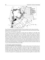
In Fig. 1 several examples of pairs of medical images prepared for comparative analysis are
shown. In the images the pairs of symmetrical regions of interest (ROIs) on which the analysis
is to be focused are marked by black rectangular contours. Note that not all differences for
comparative analysis have been chosen there; their primary selection is usually done by an
experienced medical specialist, the role of computer system is secondary, consisting in
aiding the analysis: making its results more accurate and comparable if repeated several
times.
Multi-Aspect Comparative Detection of Lesions in Medical Images

491

a) b) c)
Fig. 1. Pairs of medical images prepared for comparative analysis: a) radiological images of
knees, b) SPECT image of brain, c) microscopic image of aorta tissue.
For comparative image analysis two basic types of image features can be used:
1. Primary, local features obtained by a direct point-to-point comparison of images:
a. pixels’ intensity levels,

b. pixels’ color components.
2. Secondary, environmental features defined and calculated as functions of pixel values
in selected image fragments:
a. spectral characteristics,
b. statistical characteristics,
c. fractal characteristics,
d. micro-morphological characteristics,
etc. Local features neglect any spatial relationships between pixel values in the examined
images. It can be observed in Fig. 2 where a SPECT image of a brain a) and its mirror-
inversion b) have been subtracted in order to visualize the difference of respective pixel
intensities c). The spots in Fig. 2.c) correspond to the regions of high brightness disparities in
the compared brain hemispheres. However, no subtle differences of textures using this type
of visualization can be detected.
Environmental features take into account spatial relationships within some regular (e.g.
square or rectangular) sub-areas, called basic windows, covering the ROIs. The form of ROI is
not obviously rectangular, as shown in Fig. 3. However, identical form and size of a pair of
ROIs make their analysis easier. Black points in Fig. 3 represent image elements (pixels),
adjacent basic windows of 4×4 pixels size are separated by dotted lines, the area under


a) b) c)
Fig. 2. Result of subtraction of a SPECT brain image a) and its mirror-reflection b) visualizing
the difference of respective pixel intensities c).
examination (ROI) consisting of a compact subset of basic windows has been contoured by a
continuous line.
Biomedical Engineering, Trends, Research and Technologies

492

Fig. 3. Example of a region of interest (ROI) composed of basic windows.

An exact delineation of symmetrical pairs of ROIs needs taking both anatomical details and
measurable geometrical image parameters into consideration. Before starting a computer-
aided comparative lesions detection the images, if necessary, to a preliminary, symmetry
correcting procedure should be subjected (Lester H., Arrige S.R., 1999). However, even in
this case some remaining deficiencies of symmetry may affect the detection quality and this
in design of lesions detection procedures should be taken into consideration.
Let us take into consideration a pair A’, A” of ROIs selected for comparative analysis. There
will be denoted by M the number of basic windows in a ROI and by N be the number of
pixels in a basic window. In most medical imaging modalities, like X-ray, ultrasound (USG),
computer tomography (CT), single photon emission computer tomography (SPECT),
positron emission tomography (PET), nuclear magnetic resonance (NMR), monochromatic
images are dealt with; otherwise, pixel values should be represented by triplets of numbers
corresponding to basic, e.g. RGB, HSV, CMY, YIQ etc. color components (Foley J.D., Van
Dan A., Feiner S.K. & al., 1994). Below, monochromatic images are considered; however, the
methods presented on more general cases can easily be extended.
For comparative image analysis based on local features the contents of a pair of ROIs of
identical form and size can be represented by two M × N matrices:
U’ = [u’
μν
], U” = [u”
μν
], μ ∈ [1,…,M], ν∈ [1,…,N], (1)
where u’
μν
, u”
μν
are pixel values belonging to a finite discrete space (brightness scale):
X = [0,1,…,K–1] (2)
value 0 being assigned to the maximum darkness. We also shall denote by
u’

μ
*
= [u’
μ
1
, u’
μ
2
,…, u’
μ
N
], u”
μ
*
= [u”
μ
1
, u”
μ
2
,…, u”
μ
N
], μ ∈ [1,…,M], (3)
the respective rows assigned to the basic windows, identically enumerated in both ROIs,
and by
(u’
*
ν
)

tr
= [u’
1
ν
, u’
2
ν
,…, u’
M
ν
], (u”
*
ν
)
tr
= [u”
1
ν
, u”
2
ν
,…, u”
M
ν
], ν∈ [1,…,N], (4)
the (in transposed form presented here) columns of U’ and U”. Evidently, u’
μ
*
and u”
μ

*

represent the basic windows’ contents while u’
*
ν
and u”
*
ν
collect the related components
from the basic windows in the given ROIs.
Multi-Aspect Comparative Detection of Lesions in Medical Images

493
We consider the vectors u’
μ
*
, u”
μ
*
as elements of a N-dimensional discrete vector space X
N
.
The M-row matrices U’ and U” represent thus two M-element subsets in X
N
. The subsets
can geometrically be presented as sets of points surrounded by “clouds” (similarity areas
denoted, respectively, by
Ξ
’ and
Ξ

”) of other points (vectors) similar to those of U’ and U”,
as illustrated by Fig. 4.


a) b)
Fig. 4. Geometrical illustration of the contents of two ROIs and their similarity areas
Ξ
”,
Ξ
”:
a) easily separable (dissimilar) subsets of vectors, b) similar subsets of vectors.
For comparative lesions detection not so much vectors representing basic windows but
rather their differences
ξ
μ
*
= u’
μ
*
– u”
μ
*
are of particular interest. A condensation of difference
vectors close to the initial point of coordinates, as it is shown in Fig. 5 below, corresponds to
high similarity of basic windows contents.


a) b)
Fig. 5. Differences of pairs of vectors corresponding to the sets
Ξ

’ and
Ξ
”.
The notion of similarity area below will be more exactly defined. However, it follows from
the above-made assumption c)-ii that even if significant disparities between the similarity
areas
Ξ
’ and
Ξ
” (like those in Fig. 5 a) exist, they may be caused both by relevant as well as
irrelevant factors. Some of them (e.g. those caused by small anatomical details) by a
compensation technique can be removed. Removing other irrelevant differences needs more
sophisticated methods using as it later on will be shown. Finally, at each step of an iterative
lesions detection process it is assumed that the dissimilarities between objects within
similarity areas
Ξ
’ and
Ξ
” are mostly irrelevant while those between
Ξ
’ and
Ξ
” are mostly
relevant to the diagnostic purposes. The comparative lesions detection problem can thus
roughly be formulated as follows: