Chaotic Systems Part 6 pdf
Bạn đang xem bản rút gọn của tài liệu. Xem và tải ngay bản đầy đủ của tài liệu tại đây (3.8 MB, 25 trang )
[53] A. J. Lichtenberg and M. A. Lieberman, Regular and Stochastic Motion, Applied
Mathematical Science 38 (Springer, New York, 1983).
[54] R. Kubo, Prog. Theor. Phys., 12,570(1957).
[55] R. Kubo, M. Toda, and N. Hashitsume, Statistical Physics II: Nonequilibrium Statistical
Mechanics, Springer-Verlag, Now York 1985.
[56] R. Zwanzig, Ann. Rev. Phys. Chem. 16,67(1965).
[57] M. S. Green, J. Chem. Phys. 20,1281(1952).
[58] M. S. Green, J. Chem. Phys. 22,398(1954).
[59] R. Zwanzig, Ann. Rev. Phys. Chem. 16,67(1965).
[60] T. Marumori, T. Maskawa, F. Sakata, and A. Kuriyama, Prog. Theor. Phys. 64, 1294(1980).
[61] M. Bianucci, R. Mannella and P. Grigolini, Phys. Rev. Lett. 77, 1258(1996).
[62] E. Lutz and H. A. Weidenm
¨
uller, Physica A267, 354(1999).
[63] T. Marumori, Prog. Theor. Phys. 57, 112(1977).
[64] J. W. Negele, Rev. Mod Phys. 54, 913(1982).
[65] F. V. De Blasio, W. Cassing, M. Tohyama, P. F. Bortignon and R.A. Broglia, Phys. Rev. Lett.
68,1663(1992).
[66] A. Smerzi, A. Bonasera and M. Di Toro, Phys. Rev. C44,1713(1991).
[67] C. R. Willis and R. H. Picard, Phys. Rev. A9, 1343(1974).
[68] S. Nakajima, Prog. Theor. Phys.,20,948(1958)
[69] R. W. Zwanzig, J. Chem. Phys., 33,1338(1960).
[70] S. Y. Li, A. Klein, and R. M. Dreizler, J. Math. Phys. 11, 975(1970).
[71] A. N. Komologorov, Dokl. Akad. Nauk SSSR, 98, 527(1954).
[72] A. Bohr and B. R. Mottelson, Nuclear Structure I Benjamin, New York, 1969.
[73] W. H. Zurek and J. P. Paz, Phys. Rev. Lett. 72, 2508(1994);
W. H. Zurek, Phys. Rev. D24, 1516(1981);
E. Joos and H. D. Zeh, Z. Phys. B59, 229(1985).
[74] J. Ford, Phys. Rep. 5, 271(1992).
[75] H. Yoshida, Phys. Lett. A150, 262(1990).
[76] M. Sofroniou and W. Oevel, SIAM Journal of Numerical Analysis 34 (1997), pp.
2063-2086.
[77] N. G. van Kampen, Phys. Nor. 5, 279(1971)
[78] V. Latora and M. Baranger, Phys. Rev. Lett. 82, 520(1999).
[79] N. S. Krylov, Works on the Foundations of Statistical Physics, Princeton Series in
Physics(Princeton University Press, Princeton, NJ, 1979).
[80] P. Grigolini, M. G. Pala, L. Palatella and R. Roncaglia, Phys. Rev. E 62, 3429(2000).
[81] U. M. S. Costa, M. L. Lyra, A. R. Plastino and C. Tsallis, Phys. Rev. E 56, 245(1997).
[82] V. Latora, M. Baranger, A. Rapisarda and C. Tsallis, Phys. Lett. A273, 97(2000).
[83] C. Tsallis, Fractals 3, 541(1995).
[84] C. Tsallis, J. Stat. Phys. 52, 479(1988);
E. M. E. Curado and C. Tsallis, J. Phys. A24, L69(1991); 24, 3187E(1991); 25, 1019E(1992);
C. Tsallis,Phys. Lett. A206, 389(1995).
[85] S. Yan, F. Sakata, Y. Zhuo and X. Wu, RIKEN Review, No.23, 153(1999).
[86] F. Sakata, T. Marumori, Y. Hashimoto and T. Une, Prog. Theor. Phys. 70, 424(1983).
114
Chaotic Systems
10. Appendix
Derivation of Eq. (104)
In this appendix, a derivation of the master equation (104) is discussed. From the definition
in Eq. (103), one can get that the mean-field propagator G
η
(t, t
) satisfies the relation
dG
η
(t, t
)
dt
= −iλ
L
η
+ L
η
(t)
G
η
(t, t
) (130)
and has the properties
G
η
(t, t
1
)G
η
(t
1
, t
)=G
η
(t, t
) (131a)
G
−1
η
(t, t
)=G
η
(t
, t) (131b)
where G
−1
η
(t, t
) is the inverse propagator of G
η
(t, t
)
With the aid of the mean-field propagator, the solution of Eq. (101) can be formally expressed
as:
ρ
η
(t)=G
η
(t,0)ρ
η
(t) (132)
which satisfies the equation
˙
ρ
η
(t)=
˙
G
η
(t,0)ρ
η
(t)+G
η
(t,0)
˙
ρ
η
(t) (133)
With Eq. (130), one gets
˙
ρ
η
(t)=−iλ
L
η
+ L
η
(t)
G
η
(t,0)ρ
η
(t)+G
η
(t,0)
˙
ρ
η
(t) (134)
Inserting Eq. (132) into the r.h.s. of Eq. (101) and comparing with Eq. (134), one can easily get
˙
ρ
η
(t)=−iλL
Δ,η
(t)ρ
η
(t), (135)
where
L
Δ,η
(t)=G
−1
η
(t,0)L
Δ,η
(t)G
η
(t,0) (136)
Eq. (135) is a linear stochastic differential equation. Applying cumulant expansion
method(77), one has
˙
ρ
η
(t)=−iλL
Δ,η
(t)ρ
η
(t)
−
λ
2
t
0
dτL
Δ,η
(t)L
Δ,η
(τ)ρ
η
(t) (137)
where a symbol
···denotes a cumulant defined as:
AB≡< AB > − < A >< B > (138)
which is related to the average over the intrinsic degrees of freedom
< ···>≡ Tr{···}
115
Microscopic Theory of Transport Phenomenon in Hamiltonian Chaotic Systems
Eq. (137) is valid upto the second order in λ. According to a definition of the fluctuation
Hamiltonian H
Δ,η
(t) in (100), the first-order term in (137) is zero since there holds a relation
L
Δ,η
(t) ∼ φ
(t) = φ
(t) = 0 (139)
one thus obtains
˙
ρ
η
(t)=−λ
2
t
0
dτL
Δ,η
(t)L
Δ,η
(τ)ρ
η
(t) (140)
Inserting (140) into (134), one has
˙
ρ
η
(t)=−iλ
L
η
+ L
η
(t)
G
η
(t,0)ρ
η
(t)
−
λ
2
t
0
dτG
η
(t,0)L
Δ,η
(t)L
Δ,η
(τ)ρ
η
(t) (141)
With the relation (131), (132) and (136), Eq. (141) can be read as
˙
ρ
η
(t)=−iλ
L
η
+ L
η
(t)
ρ
η
(t)
−
λ
2
t
0
dτL
Δ,η
(t)G
η
(t, τ)L
Δ,η
(τ) G
η
(τ, t)ρ
η
(t) (142)
Making the variable transformation τ
−→ t −τ,onecanhave
˙
ρ
η
(t)=−iλ
L
η
+ L
η
(t)
ρ
η
(t)
−
λ
2
t
0
dτL
Δ,η
(t)G
η
(t, t −τ)L
Δ,η
(t −τ) G
η
(t −τ, t)ρ
η
(t) (143)
This is just Eq. (104).
116
Chaotic Systems
Part 2
Chaos Control
5
Chaos Analysis and Control in
AFM and MEMS Resonators
Amir Hossein Davaie-Markazi and Hossein Sohanian-Haghighi
School of Mechanical Engineering, Iran University of Science and Technology,
Tehran,
Iran
1. Introduction
For years, chaotic phenomena have been mainly studied from a theoretical point of view. In
the last two decades, considerable developments have occurred in the control, prediction
and observation of chaotic behaviour in a wide variety of dynamical systems, and a large
number of applications have been discovered and reported (Moon & Holmes, 1999; Endo &
Chua, 1991; Kennedy, 1993). Chaotic behaviour can only be observed in particular nonlinear
dynamical systems. In recent years, nonlinearity is known as a key characteristic of micro
resonant systems. Such devices are used widely in variety of applications, including sensing,
signal processing, filtering and timing. In many of these applications some purely electrical
components can be replaced by micro mechanical resonators. The benefits of using micro
mechanical resonators include smaller size, lower damping, and improved the performance.
Two examples of micro mechanical resonators that their complex behaviour is described
briefly in this chapter are atomic force microscopy (AFM) and micro electromechanical
resonators. AFM has been widely used for surface inspection with nanometer resolution in
engineering applications and fundamental research since the time of its invention in 1986
(Hansma et al., 1988). The mechanism of AFM basically depends on the interaction of a
micro cantilever with surface forces. The tip of the micro cantilever interacts with the surface
through a surface–tip interaction potential. One of the performance modes of an AFM is the
so called “tapping mode”. In this mode, the micro-cantilever is driven to oscillate near its
resonance frequency, by a small piezoelectric element mounted in the cantilever. In this
chapter it will be shown that micro-cantilever in tapping mode may exhibit chaotic
behaviour under certain conditions. Such a chaotic behaviour has been studied by many
researchers (Burnham et al. 1995; Basso et al., 1998; Ashhab et al., 1999; Jamitzky et al., 2006;
Yagasaki, 2007).
In section 3, the chaotic behaviour of micro electromechanical resonators is studied. Micro
electromechanical resonant systems have been rapidly growing over recent years because of
their high accuracy, sensibility and resolution (Bao, 1996). The resonators sensing
application concentrate on detecting a resonance frequency shift due to an external
perturbation such as accreted mass (Cimall et al., 2007). The other important technological
applications of mechanical resonators include radiofrequency filter design (Lin et al., 2002)
and scanned probe microscopy (Garcia et al., 1999). Many researchers have tried to analyze
nonlinear behaviour in micro electeromechanical systems (MEMS) (Mestrom et al., 2007;
Chaotic Systems
120
Younis & Nayfeh, 2003; Braghin et al., 2007). We will examine the mathematical model of a
micro beam resonator, excited between two parallel electrodes. Chaotic behaviour of this
model is studied. A robust adaptive fuzzy method is introduced and used to control the
chaotic motion of micro electromechanical resonators.
2. Atomic force microscopy
The mechanism of an AFM basically depends on the interaction of a micro cantilever with
surface forces. The tip of the micro cantilever interacts with the surface through a surface–
tip interaction potential. One of the performance modes of an AFM is the so called “tapping
mode”. In this mode, the micro-cantilever is driven to oscillate near its resonance frequency,
by a small piezoelectric element mounted in the cantilever. When the tip comes close to an
under scan surface, particular interaction forces, such as Van der Waals, dipole-dipole and
electrostatic forces, will act on the cantilever tip. Such interactions will cause a decrease in
the amplitude of the tip oscillation. A piezoelectric servo mechanism, acting on the base
structure of the cantilever, controls the height of the cantilever above the sample so that the
amplitude of oscillation will remain close to a prescribed value. A tapping AFM image is
therefore produced by recording the control effort applied by the base piezoelectric servo as
the surface is scanned by the tip.
From theoretical investigations it is known that the nonlinear interaction with the sample
can lead to chaotic dynamics although the system behaves regularly for a large set of
parameters. In this section, the model of micro cantilever sample interaction is described
and dynamical behaviour of forced system is investigated. The cantilever tip sample
interaction is modelled by a sphere of radius
R
and equivalent mass
m
which is connected
to a spring of stiffness k . A schematic of the model is shown in Fig.1. The interaction of an
intermolecular pair is given by the Lennard Jones potential which can be modelled as
(Ashhab et al., 1999)
()
()
21
7
(, )
6
1260
AR AR
VxZ
Zx
Zx
=− +
+
+
(1)
where
1
A
and
2
A
are the Hamaker constants for the attractive and repulsive potentials. To
facilitate the study of the qualitative behaviour of the system, the following parameters are
defined:
Fig. 1. The tip sample model.
R
deflection from
equilibrium position
tip
Z (the equilibrium position)
k
x
Sample
Chaos Analysis and Control in AFM and MEMS Resonators
121
()
1
1
6
21
3
00 121
2
341
,2,, , ,,,,
62 27
s
sss
AR Z A x k
DZD d t
kZAZZm
α
ζζζωτω
⎛⎞
== ==Σ= ====
⎜⎟
⎝⎠
(2)
where
t
denotes time and the dot represents derivative with respect
τ
.
Using these parameters, the cantilever equation of motion with air damping effect, is
described in state space as below
()()
12
6
00
212
28
01 01
cos
30
dd
ζζ
ζ
ζδζ τ
αζ αζ
=
Σ
=
−− − + +Γ Ω
++
(3)
where
δ
is the damping factor and
Γ
and
Ω
are the amplitude and frequency of driving force
respectively. Fig.2 shows a qualitative phase portrait of unforced system. There are two
homoclinic trajectories each one connected to itself at the saddle point.
-1.2 -1 -0.8 -0.6 -0.4 -0.2 0 0.2 0.4 0.6
-0.8
-0.6
-0.4
-0.2
0
0.2
0.4
0.6
0.8
ζ
1
ζ
2
Saddle point
Fig. 2. Phase diagram for unforced AFM model.
0 0.5 1 1.5 2 2.5
-2
-1
0
1
2
3
Γ
ζ
Fig. 3. The bifurcation diagram obtained by varying
Γ
from 0 to 2.5.
Chaotic Systems
122
For numerical simulation, we consider (3), where the parameters have been set as
follows:
αδ
Σ= = = Ω=0.3, 1.25, 0.05, 1
.For these values, the bifurcation diagram of AFM
model is shown in Fig. 3, where the parameter
Γ
is plotted versus the cantilever tip
positions in the corresponding Poincare map. The obtained diagram reveals that, starting at
Γ=1.2 , the period orbit undergoes a sequence of period doubling bifurcation. For the
range
(
)
Γ∈ 1.7, 2.5
, the system shows complex behaviours. Fig. 4 shows various types of
system responses for
Γ
= 1
,
Γ
= 1.5 and
Γ
= 2
.
0 500 1000 1500
-2
-1
0
1
2
τ
ζ
1
-2 -1 0 1 2
-2
-1
0
1
2
ζ
1
ζ
2
-2 -1 0 1 2
-2
-1
0
1
ζ
1
ζ
2
0 500 1000 1500
-2
0
2
4
τ
ζ
1
-2 0 2 4
-4
-2
0
2
4
ζ
1
ζ
2
-0.1 0 0.1 0.2 0.3
-4
-2
0
2
ζ
1
ζ
2
0 1000 2000 3000
-2
0
2
4
τ
ζ
1
-2 0 2 4
-10
-5
0
5
10
ζ
1
ζ
2
-1.5 -1 -0.5 0 0.5 1
-5
0
5
ζ
1
ζ
2
Γ
=1
Γ
=1
Γ
=1
Γ
=1.5
Γ
=1.5
Γ
=1.5
Γ
=2
Γ
=2
Γ
=2
Fig. 4. Time histories, corresponding phase diagrams and Poincare maps obtained by
simulating (3).
3. Micro electromechanical resonators
In many cases it is highly desirable to reduce the size of MEMS mechanical elements
(Roukes, 2001). This allows increasing the frequencies of mechanical resonances and
improving their sensitivity as sensors. Although miniaturized MEMS resonant systems have
many attractions, they also provide several important challenges. A main practical issue is
to achieve higher output energy, in particular, in devices such as resonators and micro-
sensors. A common solution to the problem is the well-known electrostatic comb-drive (Xie
& Fedder, 2002). However, this solution adds new constraints to the design of the
mechanical structure due to the many complex and undesirable dynamical behaviours
associated with it. Another way to face this challenge is to use a strong exciting force
(Logeeswaran et al., 2002; Harley, 1998). The major drawback of this approach is the
nonlinear effect of the electrostatic force. When a beam is oscillating between parallel
electrodes, the change in the capacitance is not a perfectly linear function. The forces
Chaos Analysis and Control in AFM and MEMS Resonators
123
attempting to restore the beam to its neutral position vary as the beam bends; the more the
beam is deflected, the more nonlinearity can be observed. In fact nonlinearities in MEMS
resonators generally arise from two distinct sources: relatively large structural deformations
and displacement-dependent excitations. Further increasing in the magnitude of the
excitation force will result in nonlinear vibrations, which will affect the dynamic behavior of
the resonator, and may lead to chaotic behaviors (Wang et al., 1998). The chaotic motion of
MEMS resonant systems in the vicinity of specific resonant separatrix is investigated based
on the corresponding resonant condition (Luo & Wang., 2002). The chaotic behavior of a
micro-electromechanical oscillator was modelled by a version of the Mathieu equation and
investigated both numerically and experimentally in (Barry et al., 2007). Chaotic motion was
also reported for a micro electro mechanical cantilever beam under both open and close loop
control (Liu et al., 2004).
In this section, the chaotic dynamics of a micro mechanical resonator with electrostatic
forces on both upper and lower sides of the cantilever is investigated. Numerical studies
including phase portrait, Poincare map and bifurcation diagrams reveal the effects of the
excitation amplitude, bias voltage and excitation frequency on the system transition to
chaos. Moreover a robust adaptive fuzzy control algorithm is introduced and applied for
controlling the chaotic motion. Additional numerical simulations show the effectiveness of
the proposed control approach.
3.1 Mathematical model
An electrostatically actuated microbeam is shown in Fig.5. The external driving force on the
resonator is applied via an electrical driving voltage that causes electrostatic excitation with
a dc-bias voltage between electrodes and the resonator:
ibAC
VVVSint
=
+Ω
, where,
b
V
is the
bias voltage, and
A
C
V
and
Ω
are the AC amplitude and frequency, respectively. The net
actuation force,
a
ct
F
, can then be expressed as (Mestrom et al., 2007)
()
2
2
00
22
11
-()
2( - ) 2( )
act b AC b
Cd Cd
FVVSintV
dz d z
=+Ω
+
(4)
where
0
C
is the capacitance of the parallel-plate actuator at rest,
d
is the initial gap width
and z is the vertical displacement of the beam. The governing equation of motion for the
dynamics of the MEMS resonator can be expressed as
Fig. 5. A schematic picture of the electrostatically actuated micromechanical resonator.
Chaotic Systems
124
3
13eff act
mz bz kz kz F
′′ ′
++ + =
(5)
where, z
′
and z
′′
represent the first and second time derivative of
z
, and
eff
m
, b ,
1
k
and
3
k
are effective lumped mass, damping coefficient, linear mechanical stiffness and cubic
mechanical stiffness of the system respectively.
It is convenient to introduce the following dimensionless variables:
2
2
0
13
0
22 22
00000
,,, , , , ,2
2
b
A
C
e
ff
e
ff
e
ff
e
ff
b
CV
zb k kd V
tx A
dm m m md V
τωω μ α β γ γ
ωωωωω
Ω
==== = = = =
(6)
where
0
ω
is the purely elastic natural frequency defined as
1
0
e
ff
k
m
ω
=
(7)
Assuming the amplitude of the AC driving voltage to be much smaller than the bias voltage,
with the dimensionless quantities defined in (6) the nondimensional equation of motion is
obtained:
3
22 2
11
(1 ) (1 ) (1 )
A
xxxx Sin
xx x
μ
αβ γ ωτ
⎛⎞
+++ = − +
⎜⎟
−+ −
⎝⎠
(8)
Here, the new derivative operator, (·), denotes the derivative with respect to
τ
. It is worth
mentioning that, if the potential is set to be zero at 0x
=
, the corresponding potential can be
described as
24
11
() 2
24 1 1
xx
Vx
xx
αβ
γ
γ
⎛⎞
=+− + +
⎜⎟
−+
⎝⎠
(9)
Fig. 6 shows that the change in the number of equilibrium points, when the applied voltage
is changed. For the case where the bias voltage does not exist, only one stable state exists,
-0.8 -0.6 -0.4 -0.2 0 0.2 0.4 0.6 0.8
-0.2
0
0.2
0.4
0.6
0.8
x
V(x)
γ
=0
γ
=0.2
γ
=0.4
γ
=0.6
Fig. 6. The potential function for four values of
γ
(
0,0.2,0.4,0.6
γ
=
), 1
α
=
and
10
β
=
.
Chaos Analysis and Control in AFM and MEMS Resonators
125
and the equilibrium point is a stable center point at x=0. When the bias voltage is not zero,
however, at a critical position, the resonator becomes unstable and is deflected against one
of the stationary transducer electrodes (pull-in phenomena). If the bias is small, the structure
stays in the deflected position, smaller than the critical one. For this case, three associated
equilibrium points are one stable center point and two unstable saddle points. As the bias
voltage increases, the equilibrium point at x=0 becomes unstable and the potential function
V(x) will have a local peak at this point. The original equilibrium point at the center position
becomes a saddle point and two new center points emerge at either side of the origin. For a
large enough bias voltage, there is only one unstable equilibrium point at x=0 and the
resonator becomes completely unstable.
3.2 Transition to chaos
To verify the analytical findings, a series of numerical simulations of the exact nonlinear
differential equation (5) is performed with the following dimensionless parameters:
3
12 8 14
13 0
5 10 , 5 10 , 5 , 15 , 2 , 1.5 10 ,mk
g
bk
g
sk N m k N m d mC F
μμ μμ μ
−− −
=× =× = = = = ×
30 , 0.5.
b
VV
ω
==
The unforced system has a saddle point at
=
0x as can be seen from Fig. 7. Existence of this
point makes homoclinic bifurcations to take place possible. This means that the system has
the necessary condition for chaotic behaviour.
The phase portrait and time histories are plotted for different values of the AC voltage. To
study the effect of the AC voltage on the beam dynamics, the bias voltage is kept fix and the
AC voltage is varied. Starting from the vicinity of the critical amplitude for
0.06
AC
VV=
, the
system response contains transient chaos and periodic motion around one of the center
points (Fig. 8a). Fig. 8b reveals that following the transient chaos, the beam oscillates in the
vicinity of the other center point for
0.17
AC
VV=
. The more increase in the AC voltage
causes a longer transient chaotic motion. The chaotic transient oscillation is large in
amplitude and jumping between potential wells. After a while in such a regime of motion, a
steady state regular vibration with much smaller amplitude, and located in a single potential
well, is observed. As can be seen from Fig. 8c, after the transient chaotic response, a periodic
motion may be observed, evolving out of the homoclinic orbit and, with much larger
-0.4 -0.3 -0.2 -0.1 0 0.1 0.2 0.3 0.4
-0.1
-0.05
0
0.05
0.1
0.15
x
y
Saddle point
Fig. 7. Phase portraits of unforced system.
Chaotic Systems
126
-0.4 -0.2 0 0.2 0.4
-0.1
-0.05
0
0.05
0.1
x
y
0 100 200 300 400 500
-0.4
-0.2
0
0.2
0.4
τ
x
-0.3 -0.2 -0.1 0 0.1 0.2 0.3
-0.1
-0.05
0
0.05
0.1
x
y
0 500 1000 1500
-0.4
-0.2
0
0.2
0.4
τ
x
0 500 1000 1500
-0.5
0
0.5
τ
x
-0.4 -0.2 0 0.2 0.4
-0.2
-0.1
0
0.1
0.2
x
y
V
AC
=0.06
V
AC
=0.17
V
AC
=0.24
(a)
(b)
(c)
Fig. 8. Phase diagrams and time histories obtained by simulating (5). Corresponding AC
voltages are indicated in phase diagrams.
amplitude. (
0.24
AC
VV=
) . With a large enough stimulation time, the system is brought back
to chaotic steady state. Fig.9 shows the phase trajectory and the Poincare map of the chaotic
motion, with
1.8
AC
VV=
. The system behavior is different from that of the Duffing attractor
because of the electrostatic terms in the MEMS equations. Because of the two unstable points
near the fixed electrodes, there is an upper limit for the applied AC voltage.
Fig. 9. The phase trajectory and the Poincare map when
1.8
AC
VV=
.
Any more increase in the AC voltage, leads to a dynamic pull-in phenomena, which could to
instability at a voltage lower than the static pull-in voltage. In interpreting the results in
Chaos Analysis and Control in AFM and MEMS Resonators
127
Fig. 10, note that
2.8
AC
VV=
corresponds to collapse of the microbeam into the fixed
electrode.
-1 -0.5 0 0.5 1
-0.5
0
0.5
x
y
0 100 200 300 400 500
-1
-0.5
0
0.5
1
τ
x
Fig. 10. The phase trajectory and time history for x(t) obtained with
2.8
AC
VV=
.
3.3 Bifurcation diagrams
Fig.11 shows the bifurcation diagram. In this case, the qualitative behavior of the system is
shown against a varying AC voltage from 0 to 2.8. In the bifurcation diagram, the final
system states of the previously iterated value of the AC voltage is chosen as the initial
condition for the next system iteration with the new value of the AC voltage. Chaotic
behavior of system starts when
1.4
AC
VV=
and continues until
2.8
AC
VV=
. For AC voltages
larger than 2.8V, the dynamic pull-in may occur, where, the electric force increases and
becomes much higher than the spring restoring force and the resonator sticks to one of the
stationary electrodes (Nayfeh &Younis, 2007). The initial conditions are assumed as
()
(,) 0,0
in in
xv =
for all simulation studies.
0 0.5 1 1.5 2 2.5 3 3.5
-0.4
-0.2
0
0.2
0.4
0.6
V
AC
(V)
x
Dynamic Pull-in
ω
=0.5, V
b
=30V
Fig. 11. The bifurcation diagram obtained by varying AC voltage from 0 to 2.8V.
The characteristic dynamical behaviors are investigated by varying the bias voltage. Fig.12
shows the bifurcation diagram of the micro beam displacement via the applied bias voltage.
The figure indicates that, with an increase in the applied bias voltage, a period-doubling
bifurcation occurs, i.e., a period-1 motion becomes a period-2 motion. If the applied bias
Chaotic Systems
128
voltage is increased, a chaotic behavoir may occur. The figure demonstrates that the chaotic
region becomes wider as the applied bias voltage is increased.
20 25 30 35
-0.4
-0.2
0
0.2
0.4
0.6
V
b
(V)
x
Dynamic Pull-in
Fig. 12. The bifurcation diagram obtained by varying the bias voltage from 20 to 32V.
0 500 1000 1500
-0.2
-0.1
0
0.1
0.2
τ
x
-0.2 -0.1 0 0.1 0.2
-0.2
-0.1
0
0.1
0.2
x
y
-0.2 -0.1 0 0.1 0.2
-0.2
-0.1
0
0.1
0.2
x
y
0 500 1000 1500
-0.4
-0.2
0
0.2
0.4
τ
x
-0.4 -0.2 0 0.2 0.4
-0.2
-0.1
0
0.1
0.2
x
y
-0.4 -0.2 0 0.2 0.4
-0.2
-0.1
0
0.1
0.2
x
y
0 1000 2000 3000
-0.5
0
0.5
τ
x
-0.5 0 0.5
-0.4
-0.2
0
0.2
0.4
x
y
-0.4 -0.2 0 0.2 0.4
-0.4
-0.2
0
0.2
0.4
x
y
V
b
=20 V
V
b
=20 V
V
b
=20 V
V
b
=25 V
V
b
=25V
V
b
=25 V
V
b
=27 V
V
b
=27 V
V
b
=27 V
Fig. 13. Time histories and corresponding phase diagrams and Poincare maps obtained by
simulating (5) with 0.5
ω
=
and
1.8
AC
VV
=
.
It can be seen from Fig. 13, that the system responses contain periodic and chaotic motions.
When
20
b
VV=
, the vibration amplitude of the cantilever is small, the period-1 motion with
only one isolated point in Poincare map and one circle in phase portrait can be observed.
With an increase in the amplitude of the applied bias voltage, the motion becomes
synchronous with period-two, as illustrated in Fig. 13 for
25
b
VV
=
. Moreover, at
27
b
VV=
,
Chaos Analysis and Control in AFM and MEMS Resonators
129
the micro beam displacement response becomes chaotic and no regular pattern can be
observed in the corresponding Poincare map and the phase portrait.
0 0.1 0.2 0.3 0.4 0.5 0.6 0.7 0.8 0.9
-0.4
-0.2
0
0.2
0.4
0.6
ω
x
Dynamic Pull-in
V
AC
=1.8 V, V
b
=30 V
Fig. 14. The bifurcation diagram obtained by varying
ω
from 0 to 0.67.
Fig. 14 shows that the system responses exhibit an alternation of periodic and chaotic
motions. The system response comes into a steady-state synchronous motion with period-1,
and returns to the chaotic motion alternatively, as the excitation frequency is increased.
Period-doubling motions are also observed for a small range of excitation frequencies.
0 5000 10000
-0.5
0
0.5
τ
x
-0.5 0 0.5
-0.2
-0.1
0
0.1
0.2
x
y
-0.5 0 0.5
-0.5
0
0.5
x
y
0 5000 10000
-0.5
0
0.5
τ
x
-0.5 0 0.5
-0.4
-0.2
0
0.2
0.4
x
y
-0.4 -0.2 0 0.2 0.4
-0.4
-0.2
0
0.2
0.4
x
y
0 1000 2000 3000 4000
-0.5
0
0.5
τ
x
-0.5 0 0.5
-0.2
-0.1
0
0.1
0.2
x
y
-0.5 0 0.5
-0.2
-0.1
0
0.1
0.2
x
y
ω
=0.1
ω
=0.27
ω
=0.35
ω
=0.27
ω
=0.27
ω
=0.35
ω
=0.1
ω
=0.1
ω
=0.35
Fig. 15. Time histories, corresponding phase diagrams and Poincare maps obtained by
simulating (5) with
30
b
VV
=
and
1.8
AC
VV
=
.
Chaotic Systems
130
Fig. 15 depicts the time history, phase plane portraits and the Poincare maps based on the
responses of the electrostatically actuated system over a range of frequencies. Various
chaotic behavior is observed for 0.2
ω
=
and 0.27
ω
=
. It can be seen that, for 0.35
ω
= , the
motion of the system is synchronized with period-one.
3.4 Control of chaotic motion in MEMS resonator
Various fuzzy control methods for control of chaotic systems are proposed in the literature
e.g., (Calvo, 1998; Poursamad & Markazi, 2009-a; Haghighi & Markazi, 2010). In this section,
a robust adaptive fuzzy control algorithm is used to stabilize a MEMS beam in a high-
amplitude oscillation state. A key issue that arises in chaos control, particularly in MEMS
resonators, is that the system parameters are not known precisely, and are perturbed during
operation (Wang et al., 1998). Unlike most conventional control systems whose equilibriums
are assumed known and fixed regardless of values of the system parameters, the
equilibriums of chaotic systems are a function of their system constant parameters. This
suggests that, when the system parameters are not precisely known, and hence, the
equilibriums are then unknown, the conventional control methodologies may not be applied
directly. In addition, the presence of external disturbance and measurement noise, may
adversely affect the system performance. Therefore, development of alternative control
strategies for efficient control and robust tracking of chaotic systems, under the presence of
uncertainties is highly desirable.
The controller proposed in this section comprises a fuzzy system and a robust controller.
The fuzzy system, whose parameters are adaptively tuned, is designed based on the sliding-
mode control (SMC) strategy to mimic the ideal controller, i.e., when the model of the plant
is exactly known. The robust controller is then designed to compensate for deviations of the
fuzzy controller, compared to the ideal one. The uncertainty bound needed in the robust
controller is also adaptively tuned online to avoid using unnecessary high switching gain,
due to the, most often, conservative bounds. A comprehensive presentation of the proposed
control method and proof of the asymptotic stability can be found in (Poursamad &
Markazi, 2009-a ; Poursamad & Markazi, 2009-b).
In order to write (5) in a more convenient form, it is rewritten as
(,,)xfxxtu
=
+
, (10)
where
u
is the appended control input and
f
is a smooth function obtained from (5). Now
let define a sliding surface,
()St
, using
(,) 0sxx
=
with
(,)sxx x x=+
λ
, where
d
xx x=−
is the
tracking error,
x
is the time derivative of
x
,
d
x
is the desired trajectory and
λ
is a to be
selected strictly positive constant. Now, an ideal (central) control signal is obtained as
d
u
f
xx
λ
∗
=− + +
(11)
and the control law is defined as
rb
uu u
∗
=+
, (12)
where, the robust control signal,
rb
u , is designed to overcome the deviations from the
sliding surface, by employing a switching strategy:
Chaos Analysis and Control in AFM and MEMS Resonators
131
s
g
n( )
rb
us
δ
=
(13)
Here,
δ
is the bound of uncertainties. It is noted that, in the design of a conventional SMC,
the uncertainty bound
δ
, must be known or estimated at the outset of the control design, a
matter which is not easily achievable in practice. Such uncertainties may include unknown
plant dynamics, parameter variations, and external load disturbances. In particular, the
dynamics of micro/nano electromechanical systems are not known exactly, so the ideal
controller proposed in (11) may not actually work in practice. As an alternative, the ideal
controller can be approximated by a fuzzy inference system
(
)
ˆ
T
uBWs
ψ
∗
=
+
(14)
Here,
ˆ
B
is the estimated value for the optimal weighting vector, and
[]
1
T
n
Ww w= "
is a
vector with components
1
()
n
rr r
r
ws
μ
μ
=
=
∑
and, where,
r
μ
is the firing strength of the
th
r
rule of the fuzzy algorithm. The bias term
ψ
represents unmodeled dynamics and external
disturbances and is assumed to be bounded as
ψ
ψ
≤
. The weighting vector can be updated
by the adaptation rule
1
ˆ
()BstW
α
=
, and the bound of uncertainties is estimated by the
adaptation rule
ψα
=
2
()st
, where
1
α
and
2
α
are strictly positive constants, adaptation rates.
-3 -2 -1 0 1 2 3
0
0.2
0.4
0.6
0.8
1
s
Membership degree
Zero
Negative
Positive
Fig. 16. Membership functions of
s
for robust adaptive fuzzy control.
The objective is to control the position variable
x
so as to track the desired
trajectory
0.6sin 0.5
d
x
τ
=
. The resonator properties are the same as introduced in Section 3.2
and
1.8
AC
VV=
. The input membership functions are selected as shown in Fig. 16 and the
sliding surface is defined as
sxx
=
+
. The parameters of these membership functions are
chosen such that the parameter
s
remains close to zero. The initial weighting vector is
arbitrarily selected as
[]
ˆ
101
T
B =
, the initial value of the uncertainty bound is chosen
as
0.01
ψ
=
and the learning rates are set to
1
1
α
=
and
4
2
210
α
−
=×
. The controller is
activated at 200=
τ
, for which the resulting output is depicted in Fig. 17, showing the
effectiveness of the proposed control strategy.
Chaotic Systems
132
0 50 100 150 200 250 300
-1
-0.5
0
0.5
1
τ
x
0 50 100 150 200 250 300
-1
0
1
2
3
4
τ
Control effort
Control on
Control off
Desired response
System response
Fig. 17. Simulation results for MEMS resonator with proposed control strategy.
4. Conclusions
This chapter deals with the chaotic motion of micromechanical resonators. The source of
nonlinearities in AFM is the Lennard Jones force while nonlinearities in MEMS resonator
system include mechanical nonlinearity due to large deformation and nonlinear electrostatic
forces. It is shown that each of these systems has one unstable fix point that connects the
corresponding homoclinic trajectory to itself. Certain set of parameters may cause
homoclinic bifurcation in these systems. Such a bifurcation corresponds to double periodic
behavior of the system. It is seen that increase in the amplitude of driving force could lead to
a chaotic motion. Finally, an adaptive fuzzy-sliding mode strategy was proposed for control
of the chaotic motion. It was shown through simulations study that such a control strategy
could successfully eliminate the chaotic motion and force the system response towards a
stable orbit.
5. References
Ashhab, M. ; Salapaka, M.V.; Dahleh, M. & Mezic, I. (1999). Dynamical analysis and control
of micro-cantilevers, Automatica, Vol. 35 , pp. 1663–1670.
Barry, E.; DeMartini, B. E.; Butterfield, E. ; Moehlis, J. & Turner, K. (2007). Chaos for a
Microelectromechanical Oscillator Governed by the Nonlinear Mathieu Equation,
Journal of Microelectromechanical Systems, Vol. 16, pp. 1314–1323.
Basso, M.; Giarrk, L.; Dahleh, M. & Mezic, I. (1998). Numerical analysis of complex
dynamics in atomic force microscopes, Proc. IEEE Int. Conf. Control Appl.
Burnham, N.A. ; Kulik, A.J. ; Gremaud, G. & Briggs, G.A.D. (1995). Nanosubharmonics: The
dynamics of small nonlinear contacts, Phys. Rev. Lett., Vol. 74, pp. 5092–5059.
Calvo, O. (1998), Fuzzy control of chaos, International Journal of Bifurcation and Chaos, Vol. 8,
No. 8, pp 1743–1747.
Chaos Analysis and Control in AFM and MEMS Resonators
133
Chacon, R. (1999). General results on chaos suppression for biharmonically driven
dissipative systems. Phys Lett A; 257, pp. 293–300.
Endo, T. & Chua, L. O. (1991). Synchronization of chaos in phase-locked loops, IEEE Trans.
Circuits Syst., Vol. 38, pp. 1580-1588.
Garcia, R.; Tamayo, J. & San Paulo, A. (1999). Phase contrast and surface energy hysteresis
in tapping mode scanning force microscopy, Surface Interface Anal 27, pp.312–316.
Haghighi, H.S. & Markazi, A.H.D. (2010), Chaos prediction and control in MEMS
resonators, Commun Nonlinear Sci Numer Simulat, Vol. 15, pp. 3091–3099.
Hansma, P.K. ; Elings, V.B. ; Marti, O. & Bracker, C.E. (1988). Scanning tunneling
microscopy and atomic force microscopy: Application to biology and technology,
Science, Vol. 242 , pp. 209-242.
Harley, J.A. ; Chow, E.M. & Kenny, T.W. (1998). Design of resonant beam transducers: An
axial force probe for atomic force microscopy, In Micro-Electro-Mechanical Systems:
ASME Intl. ME Congress and Exposition, pp 274-252, Anaheim, Ca.
Jamitzky, F.; Stark, M.; Bunk, W. ; Heckl, W.M. & Stark, R.W. (2006). Chaos in dynamic
atomic force microscopy, Nanotechnology, Vol. 17 pp. 213–220.
Kennedy, M. P. (1993). Three steps to chaos, Part I: Evolution, Part II: A Chua’s circuit
primer, IEEE Trans. Circuits Syst. I, Vol. 40, No.10, pp.640-656.
Lin, L.; Howe, R. & Pissano, A.P. (1998). Microelectromechanical filters for signal processing,
J. Microelectromech. Syst. Vol. 7, No.3, pp. 286–294.
Liu, S; Davidson, A; & Lin, Q. (2004). Simulation studies on nonlinear dynamics and chaos
in a MEMS cantilever control system, Journal of Micromechanics and
Microengineering,Vol. 14, pp. 1064–1073.
Logeeswaran, V.J.; Tay, F.E.H.; Chan, M.L.; Chau, F.S. & Liang, Y.C. (2002). Proceedings of the
DTIP 2002 on A 2f Method for the Measurement of Resonant Frequency and Q-factor of
Micromechanical Transducers, ,pp. 584–590, Cannes, May 2002.
Luo, A. & Wang Fei-Yue. (2002). Chaotic motion in a micro-electro-mechanical system with
non-linearity from capacitors, Commun Nonlinear Sci Numer Simul, Vol. 7, pp. 31–49.
Melnikov, VK. (1963). On the stability of the center for time periodic perturbations. Trans
Moscow Math Soc,12, pp. 1–57.
Mestrom, R.M.C. ; Fey, R.H.B.; van Beek, J.T.M.; Phan, K.L. & Nijmeijer, H. (2007).
Modeling the dynamics of a MEMS resonator: Simulations and experiments, Sens.
Actuators A, Vol. 142 ,pp. 306-315.
Moon, F. C. & Holmes, P. A magnetoelastic strange attractor, J. Sound Vib., Vol. 65, No. 2,
pp. 285–296.
Nayfeh, A.H.; Younis, M.I.; Abdel-Rahman, E. (2007). Dynamic pull-in phenomenon in
MEMS resonators, Nonlinear Dynamics,Vol. 48,pp. 153-63.
Poursamad, A. & Davaie-Markazi, A.H. (2009-a). Robust adaptive fuzzy control of
unknown chaotic systems, Applied Soft Computing, Vol. 9, pp. 970–976.
Poursamad, A. & Markazi, A.H.D. (2009-b) Adaptive fuzzy sliding-mode control for multi-
input multi-output chaotic systems, Chaos, Solitons Fractals, Vol. 42, pp. 3100–3109.
Roukes, M. (2001). Nanoelectromechanical systems face the future, Phys.World, Vol. 14 , pp.
25.
Wang, Y.C.; Adams, S.G.; Thorp, J.S.; MacDonald, N.C.; Hartwell, P. & Bertsch, F. (1998).
Chaos in MEMS, parameter estimation and its potential application, IEEE Trans.
Circuits Syst. I, Vol. 45, pp. 1013–1020.
Chaotic Systems
134
Xie, H. & Fedder, G. (2002). Vertical comb-finger capacitive actuation and sensing for coms-
MEMS, Sens. Actuators A, Vol. 95 , pp. 212–221.
Yagasaki, K. (2007), Bifurcations and chaos in vibrating microcantilevers of tapping mode
atomic force microscopy, Journal of Non-Linear Mechanics, Vol. 42, pp. 658 – 672.
Younis, M. I. & Nayfeh, A. H. (2003). A Study of the Nonlinear Response of a Resonant
Microbeam to an Electric Actuation, Nonlinear Dynamics, Vol. 31, No. 1 pp. 91–117.
0
Control and IdentiÀcation of Chaotic Systems by
Altering the Oscillation Energy
Valery Tereshko
University of the West of Scotland
United Kingdom
1. Introduction
Last years, researchers paid a major attention to the controlling chaos schemes that use
information obtained from the experimental time series of system’s accessible variables.
When the trajectory is in a neighbourhood of desired UPO, the Ott-Grebogi-Yorke (OGY)
controlling chaos scheme can be applied (Ott et al., 1990). Exploiting the linearity of return
map near corresponding unstable fixed point, it stabilizes UPOs with one unstable direction
by directing the trajectory to the orbit stable manifold. The technique requires performing
several calculations to generate a control signal. This approach may fail (i) if the dynamics is
so fast that the controller cannot follow it, and (ii) if the dynamics is highly unstable, i.e. the
trajectory diverges from a target so far that small perturbations cannot be effective. For highly
dissipative systems that are well characterized by a one-dimensional return map, occasional
proportional feedback (Hunt, 1991; Peng et al., 1991) and occasional feedback (Myneni et al.,
1999) techniques was developed. The occasional proportional feedback utilizes an amplitude
of parametric perturbation that is proportional to the deviation of system’s current state from
its desired state (Hunt, 1991; Peng et al., 1991). Similar technique but with application to a
system accessible variable instead of a parameter is called proportional perturbation feedback
(Garfinkel et al., 1992). Alternatively, occasional feedback utilizes a control pulse duration that
is equal to the transit time of trajectory through a specified window placed on either side of
saddle fixed point (Myneni et al., 1999). Owing to simplicity, these methods do not require
any processor and can be implemented at high speeds.
For highly unstable orbits, quasicontinuous extensions of original OGY technique can be
applied when more than one control points per period are taken (Hübinger et al., 1994; Reyl
et al., 1993). Another option is to use a continuous-time control (Gauthier et al., 1994; Just et
al., 1999b; Pyragas, 1992; 1995; Socolar et al., 1994). However, obtaining complete information
about desired trajectory can be difficult (or even impossible, say, at high frequencies or spatial
complexity). Therefore, the continuous-time delayed feedback using information only about
a period of desired UPO became most popular. Here, the control signal is proportional to the
difference between a system current state and its state at some earlier time, the delay being
set to a period of desired UPO (Gauthier et al., 1994; Pyragas, 1992). This approach is found
effective to control low-period UPOs at high frequencies (Gauthier et al., 1994), but it may
fail for high-period UPOs or for highly unstable orbits (Just et al., 1999b). An extension of
method that incorporates information from many previous states of the system is suitable for
controlling UPOs in fast dynamical systems, with large value of Lyapunov exponents, and of
6
high periods (Socolar et al., 1994). The attractiveness of delayed feedback scheme consists in
the self-organizing ability of a system to autosynchronize its own behaviour. However, unlike
the OGY-based schemes where the trajectory is targeted to a predefined UPO, the delayed
feedback control does not discriminate between different periodic orbits of the same period,
and does not necessarily lead to the stabilization of orbits embedded in a chaotic attractor
(Hikihara et al., 1997; Simmendinger et al., 1998). The success of this control is significantly
restricted by a control loop latency (Just et al., 1999a).
In the nonfeedback, or open-loop, schemes, the control signal does not depend on a system
state. One of approaches is a nonlinear entrainment method (Hübler & Lüscher, 1989; Jackson
& Hübler, 1990). It requires knowledge of the system equations to construct control forces
that can have large amplitude and complicated shape. The basins of entrainment, in turn, can
have very complicated structure. Typically, this method can require as many control forces, as
there are dimensions of the system.
In contrast, there are many examples of converting chaos to a periodic motion by exposing a
system to only one, weak periodic force or weak parameter modulation (Alexeev & Loskutov,
1987; Braiman & Goldhirsch, 1991; Cao, 2005; Chacón, 1996; Chacón & Díaz Bejarano, 1993;
Chizhevsky & Corbalán, 1996; Chizhevsky et al., 1997; Dangoisse et al., 1997; Fronzoni et al.,
1991; Kivshar et al., 1994; Lima & Pettini, 1990; Liu & Leite, 1994; Meucci et al., 1994; Qu et al.,
1995; Ramesh & Narayanan, 1999; Rödelsperger et al., 1995; Tereshko & Shchekinova, 1998).
Typically, this approach utilizes only a period and an amplitude of perturbation (Alexeev &
Loskutov, 1987; Braiman & Goldhirsch, 1991; Kivshar et al., 1994; Lima & Pettini, 1990; Liu &
Leite, 1994; Ramesh &Narayanan, 1999). If the amplitude is kept small enough, one can expect
a controlled periodic orbit or an equilibrium to trace closely the corresponding unperturbed
one (provided that no crises are induced). The periodic perturbation methods can be easily
realized in practice. However, the independence of the perturbation from a system state leads
to some limitations of above approach: the control by periodic perturbations relying only on
their period and amplitude is not, in general, a goal-oriented technique (Shinbrot et al., 1993).
On the other hand, the importance of a phase (Cao, 2005; Chacón, 1996; Chizhevsky &
Corbalán, 1996; Chizhevsky et al., 1997; Dangoisse et al., 1997; Fronzoni et al., 1991; Meucci
et al., 1994; Qu et al., 1995; Tereshko & Shchekinova, 1998) and even a shape (Azevedo
& Rezende, 1991; Chacón, 1996; Chacón & Díaz Bejarano, 1993; Rödelsperger et al., 1995)
of perturbation became evident. The utilization of extra parameters allows tuning the
perturbation to a desired target shape more selectively. The above findings were generalized
in a concept of geometrical resonance that reveals the underlying mechanism of nonfeedback
resonant control for a general class of chaotic oscillators (Chacón, 1996). The phase of
perturbation is crucial for the success of nonfeedback resonant control. First of all, it
determines the direction and, hence, the targets where a trajectory is driven to. Secondly,
keeping the perturbation precisely in phase with the controlled signal ensures smallest control
amplitudes, whereas dephasing can destroy the control. By changing only the perturbation
phase, one can switch the trajectory from one controlled state to another (Tereshko &
Shchekinova, 1998).
In real-life systems, the existing uncontrolled drifts can spoil resonant conditions. Small
deviation of the perturbation frequency from the resonance is equivalent to slowly varying
modulation of the phase. This results in a temporal evolution consisting of regular alternations
between a stabilized orbit and the chaotic behaviours (Chizhevsky & Corbalán, 1996; Meucci
et al., 1994; Qu et al., 1995). The real-life nonfeedback control may, thus, demand an occasional
136
Chaotic Systems
adjustment of the perturbation frequency. To overcome the above problem, a feedback control
where the perturbation depends on the controlled signal can be used.
Have analyzed the existing approaches, we developed a following control method. To any
type of system behaviour, we put in correspondence a value of averaged oscillation energy
that is an averaged (over the time) compound of the system kinetic and potential energy.
The objective is to alter this energy so as to correspond to a desired behaviour. This is a
general approach that does not depend on particular oscillator equations. Simple feedback
depending solely on an output signal is utilized for this purpose. We start with identifying
the type of control perturbations appropriate for the above control. One simply increases the
feedback strength, and, thus, depending on the perturbation phase, increases or decreases
the oscillation energy. The above strategy does not require any computation of the control
signal and, hence, is applicable for control as well as identification of unknown systems. The
above approach was applied to control isolated oscillators, as well as coupled ones (Tereshko,
2009; Tereshko et al., 2004a;b). Here, we summarize the obtained results and present our new
findings in controlling spatially-extended systems.
2. General approach
Let us consider controlling a general type nonlinear oscillator
¨
x
+ χ(x,
˙
x)+ξ(x)=F(t)+g(x,
˙
x) (1)
where χ
(x,
˙
x), ξ(x) and g(x,
˙
x) are dissipative or energy-generating component, restoring
force, and control force, respectively. These functions are nonlinear in general case. Also,
χ
(x,
˙
x) and g(x) are assumed not to contain an additive function of x. F(t) is an external
time-dependent driving force.
At F
(t)=0andg(x,
˙
x)=0, Eq. (1) possesses the equilibriums defined by equation
ξ
(x)=0. In oscillators with nonlinear damping (say, van der Pol and Reyleigh oscillators), an
equilibrium becomes unstable at some parameter values, and stable self-sustained oscillations
are excited. In other types of oscillators, say Duffing oscillator, a limit cycle arises under the
action of periodic driving force. We assume that at some driving amplitudes, a limit cycle
becomes saddle, and new attractor, say period-2 cycle, arises. In many well-known examples,
this scenario leads, through the sequence of bifurcations, to the birth of chaotic attractor.
One can define an energy of oscillations as the sum of “potential" and “kinetic" energy:
E
(t)=
ξ(x) dx +
1
2
˙
x
2
.(2)
An averaged (over period T) energy yields
E =
1
T
T
0
ξ(x) dx +
1
2
˙
x
2
dt .(3)
For periodic dynamics T is an oscillation period, whereas for chaotic one T
→ ∞.Each
attractor of an oscillator is assigned to a value of averaged energy (3). If an oscillation
amplitude is sufficiently small, the limit cycle oscillations can be approximated as x
ρ sinωt,
which gives
E =
1
2
ρ
2
.
Typically, transitions to a chaotic attractor correspond to the increase of energy (3). Let us
clarify this statement on the example of a period-doubling process. Suppose that changing
some of the system parameters results in an oscillation period doubling and, eventually, in a
137
Control and Identification of Chaotic Systems by Altering the Oscillation Energy
chaos. Starting at period-1 cycle, its amplitude grows with increasing the above parameter,
and, hence, energy (3) does. Every period-doubling bifurcation contributes subharmonic (as
well as its odd harmonic) to the fundamental frequency, which again increases energy (3).
Thus, the higher the orbit period is, the higher the averaged energy correspondingto this orbit.
A stationary point, around which a limit cycle develops, can be viewed as a zero-amplitude
cycle possessing, thus, zero energy.
A following control strategy can be proposed. Starting at a lower energy attractor, one
stabilizes higher energy repellors by sequential increasing the averaged oscillation energy.
On the contrary, decreasing this energy leads to the stabilization of lower energy repellors.
A change of energy (2) yields
˙
E
(t)=ξ(x)
˙
x
+
˙
x
¨
x
=
−χ(x,
˙
x)+F(t)+g(x,
˙
x)
˙
x .(4)
The last term of (4) represents an energy change caused solely by the control. We require that
g
(x,
˙
x)
˙
x
> 0 (< 0) (5)
for
∀(x,
˙
x). A minimal feedback satisfying (5) is achieved at g = g(
˙
x
). Indeed, simple linear
(relative to the velocity) control g
(
˙
x
) ∼
˙
x as well as nonlinear controls of higher power, say
g
(
˙
x
) ∼
˙
x
3
suffice. In general
g
(
˙
x
)=kh(
˙
x
) (6)
where h
(
˙
x
) is assumed to be odd, i.e. h(
˙
x
)=− h(−
˙
x
). One can, thus, define
h
(
˙
x
)
⎧
⎪
⎨
⎪
⎩
> 0, if
˙
x > 0
= 0, if
˙
x = 0
< 0, if
˙
x < 0.
(7)
To guarantee a control perturbation tininess even at high values of
˙
x, h
(
˙
x
) is taken to be
bounded. Throughout, we consider g
(
˙
x
)=k tanh(β
˙
x) with 0 < β ∞ determining the
function slope.
Perturbation (6-7) is specially tuned to control equilibriums: their positions are not changed
by the control as the latter vanishes at
˙
x
= 0.
˙
E = 0 at equilibriums respectively. The above
control does not vanish at dynamic attractors. Our aim, however, is not controlling the UPOs
of unperturbed system existing at given parameter values, but rather the shift of a system into
a region of desired behaviours. Energy (3) is changed so as to match energy of a desired state.
For small oscillations, one can find amplitude ρ by substituting x
= ρ sinωt into an averaged
(over period T) energy change and solving equation
˙
E
=
1
T
T
0
˙
E
(t) dt =
1
T
T
0
−χ(x,
˙
x)+F(t)+g(x,
˙
x)
˙
x dt
= 0. (8)
Equation (8) describes the balance of dissipation and energy supply brought by damping,
driving, and control forces. For general orbit defined by the infinite series of periodic modes,
a fundamental mode as well as its harmonics should, in principle, be counted.
In this paper, we alter the feedback strength to adjust the oscillation energy to different
levels. The above strategy does not require any computation of control signal and, hence,
is applicable for control as well as identification of unknown systems.
138
Chaotic Systems