Data Acquisition Part 4 ppt
Bạn đang xem bản rút gọn của tài liệu. Xem và tải ngay bản đầy đủ của tài liệu tại đây (2.23 MB, 30 trang )
Real Time Data Acquisition in Wireless Sensor Networks
81
communication task, e.g. medium access or routing, we also present comparisons of them.
These comparisons provide a snapshot view of the protocols and derive conclusions on how
new approaches should be. Of the routing protocols, Stateless Weighted Routing (SWR) is
one key protocol that aims to solve multiple objectives and problem in WSN. With respect to
other protocols, SWR is the easiest and the simplest one to implement. It has many
advantages and is superlative compared to other similar protocols.
While aggregation approaches are needed to reduce communication overhead, to provide
efficient bandwidth usage, and to provide higher quality data, these approaches introduce
delay. Moreover, aggregation is a complex task to be handled in identical tiny sensor nodes.
Aggregation at more powerful nodes (with additional ability and higher resources) is more
attractive solution.
There are applications that use real-time data aggregation via Wireless Sensor Networks.
Of these, we present two and give design strategies of them. By increased demand on
sensor applications, applications that use real-time data aggregation via WSN will increase
in near future.
8. References
Akkaya K. and M. Younis, (2004) "Energy-aware routing of time-constrained traffic in
wireless sensor networks," in the International Journal of Communication Systems,
Special Issue on Service Differentiation and QoS in Ad Hoc Networks, 2004
Akkaya K., M. Younis, and M. Youssef, (2005) “Efficient aggregation for delay-constrained
data in wireless sensor networks”, The Proceedings of Internet Compatible QoS in Ad
Hoc Wireless Networks, 2005.
Akyildiz I. F., W. Su , Y. Sankarasubramaniam , E. Cayirci, (2002) “Wireless sensor
networks: a survey”, Computer Networks: The International Journal of Computer and
Telecommunications Networking, v.38 n.4, p.393-422, 15 March 2002
Ali A., LA Latiff, MA Sarijari, N. Fisal,” (2008) Real- time Routing in Wireless Sensor
Networks”, The 28th International Conference on Distributed Computing Systems
Workshops, 2008, pp 114- 119.
Al-Karaki JN, AE Kamal, (2004) “Routing techniques in wireless sensor networks: a survey”,
IEEE Wireless Communications, 2008
Annamalai V., S. K. Gupta and L. Schwiebert. (2003) On Tree-Based Convergecasting in
Wireless Sensor Networks. IEEE Wireless Communications and Networking Conference
2003, New Orleans.
Bacco, G.D., T. Melodia and F. Cuomo, (2004) “A MAC protocol for delay-bounded
applications in wireless sensor networks” Proc. Med-Hoc-Net. pp. 208-220.
Caccamo, M., L.Y. Zhang, L. Sha and G. Buttazzo, (2002) “An implicit prioritized access
protocol for wireless sensor networks”, Proc. 23rd IEEE RTSS. pp. 39-48.
Chen M, Leung VCM,Mao S, Yuan Y. (2007) Directional geographical routing for real-time
video communications in wireless sensor networks. Elsevier Computer
Communications 2007.
Cheng H, Q Liu, X Jia (2006) “Heuristic Algorithms for Real-time Data Aggregation in
Wireless Sensor Networks”, IWCMC’06, July 3–6, 2006, Vancouver, British
Columbia, Canada.
Data Acquisition
82
Cheng W, L Yuan, Z Yang, X Du, (2006), “A Real-time Routing Protocol with Constrained
Equivalent Delay in Sensor Networks”, Proceedings of the 11th IEEE Symposium on
Computers and Communications (ISCC'06)
Chenyang Lu , Brian M. Blum , Tarek F. Abdelzaher , John A. Stankovic , Tian He, (2002)
RAP: A Real-Time Communication Architecture for Large-Scale Wireless Sensor
Networks, Proceedings of the Eighth IEEE Real-Time and Embedded Technology and
Applications Symposium (RTAS'02), p.55, September 25-27, 2002
Chipara O., Z. He, G. Xing, Q. Chen, X. Wang, C. Lu, J. Stankovic, and T. Abdelzaher. (2006)
Real-time Power Aware Routing in Wireless Sensor Networks. In IWQOS, June
2006
Chipcon. CC2420 low power radio transceiver, .
Chlamtac I. and S. Kutten. (1987) Tree-based Broadcasting in Multihop Radio Networks.
IEEE Transactions on Computers Vol. C-36, No. 10, Oct 1987.
Demirkol I, C Ersoy, F Alagoz, “MAC protocols for wireless sensor networks: a survey”,
(2006) IEEE Communications Magazine.
Du H. X. Hu, X. Jia, “Energy Efficient Routing And Scheduling For Real-Time Data
Aggregation In WSNs”, Computer Communications, vol.29 (2006) 3527–3535
Felemban E., C G. Lee, E. Ekici, R. Boder, and S. Vural, (2005) "Probabilistic QoS Guarantee
in Reliability and Timeliness Domains in Wireless Sensor Networks," in Proceedings
of IEEE INFOCOM 2005, Miami, FL, USA.
Ergen, S.C. and P. Varaiya (2006). PEDAMACS: power efficient and delay aware medium
access protocol for sensor networks. IEEE Trans. Mobile Comput. 5(7), 920-930.
Francomme, J., G. Mercier and T. Val (2006).A simple method for guaranteed deadline of
periodic messages in 802.15.4 cluster cells for control automation applications. In:
Proc.IEEE ETFA. pp. 270-277.
He T., J. Stankovic, C. Lu, T. Abdelzaher, (2003) SPEED: A real-time routing protocol for
sensor networks, in: Proc. IEEE Int. Conf. on Distributed Computing Systems (ICDCS),
Rhode Island, USA, May 2003, pp. 46–55.
He T., P. A. Vicaire, T. Yan, L. Luo, L. Gu, G. Zhou, R. Stoleru, Q. Cao, J. A. Stankovic, and T.
Abdelzaher, (2006) “Achieving real-time target tracking using wireless sensor
networks.” in RTAS’06.
He, T., L. Gu, L. Luo, T. Yan, J. Stankovic, T. Abdelzaher and S. Son (2006b). An overview of
data aggregation architecture for real-time tracking with sensor networks. In: Proc.
IEEE RTAS. pp. 55-66.
Heinzelman W., A. Chandrakasan, and H. Balakrishnan, (2000), “Energy -Efficient
Communication Protocol for Wireless Microsensor Networks,” In Proceedings of the
Hawaii Conference on System Sciences, Jan. 2000.
Heinzelman W., A. Chandrakasan, and H. Balakrishnan, (2000), Energy-Efficient
Communication Protocol for Wireless Sensor Networks, Proceeding of the Hawaii
International Conference System Sciences, Hawaii, USA, January 2000.
Hu Y, N Yu, X Jia, (2006) “Energy efficient real-time data aggregation in wireless sensor
networks ” IWCMC’06, July 3–6, 2006, Vancouver, British Columbia, Canada.
IEEE Std 802.15.4 (2006). Part 15.4: Wireless medium access (MAC) and physical layer (PHY)
specifications for low-rate wireless personal area networks (WPANs). IEEE-SA.
Real Time Data Acquisition in Wireless Sensor Networks
83
Jamieson K., H. Balakrishnan, and Y. C. Tay, (2003) “Sift: A MAC Protocol for Event-Driven
Wireless Sensor Networks,” MIT Laboratory for Computer Science, Tech. Rep. 894,
May 2003
Kim T.H. and S. Choi (2006). Priority-based delay mitigation for event-monitoring IEEE
802.15.4 LR-WPANs. IEEE Commun. Letters 10(3), 213-215.
Koubaa A., M. Alves, B. Nefzi and Y. Q. Song (2006). Improving the IEEE 802.15.4 slotted
CSMA/CA MAC for time-critical events in wireless sensor networks. In: Proc.
Workshop Real-Time Networks. pp. 270-277.
Krishnamachari L, D Estrin, S Wicker, (2002), “Impact of Data Aggregation in Wireless
Sensor Networks”, Distributed Computing Systems Workshops, 2002
Langendoen K, Medium access control in wireless sensor networks. In H. Wu and Y. Pan,
editors, (2007) Medium Access Control in Wireless Networks, Volume II: Practice and
Standards. Nova Science Publishers, Inc.
Li, Y.J.; Chen, C.S.; Song, Y Q.; Wang, Z. (2007) Real-time QoS support in wireless sensor
networks: a survey. In Proc of 7th IFAC Int Conf on Fieldbuses & Networks in Industrial
& Embedded Systems (FeT'07), Toulouse, France.
Lin P., C. Qiao, and X. Wang, (2004) “Medium access control with a dynamic duty cycle for
sensor networks”, IEEE Wireless Communications and Networking Conference,
Volume: 3, Pages: 1534 - 1539, 21-25 March 2004.
Lu C., G. Xing, O. Chipara, C L. Fok, and S. Bhattacharya, (2005) “A spatiotemporal query
service for mobile users in sensor networks,” in ICDCS ’05.
Lu C., B.M. Blum, T.F. Abdelzaher, J.A. Stankovic and T. He (2002). RAP: a real-time
communication architecture for large-scale wireless sensor networks. In: Proc. IEEE
RTAS. pp. 55-66.
Lu G., B. Krishnamachari and C.S. Raghavendra, (2004) “An adaptive energy-efficient and
low-latency MAC for data gathering in wireless sensor networks” Proc. Int. Parallel
Distrib. Process. Symp. pp. 224-231.
Monaco U., et.al. “Understanding Optimal Data Gathering In the Energy and Latency
Domains of A Wireless Sensor Network”, Computer Networks, vol. 50 (2006) 3564–
3584
Otero Carlos E., Antonio Velazquez, Ivica Kostanic, Chelakara Subramanian, Jean-Paul
Pinelli,(2009) "Real-Time Monitoring of Hurricane Winds using Wireless and
Sensor Technology", Journ. of Comp
Raghunathan V., C. Schurgers, S. Park, and M. B. Srivastava, (2002) “Energyaware wireless
microsensor networks,” IEEE Signal Processing Mag., vol. 19, no. 2, pp. 40–50, Mar.
2002.
Rajagopalan R, PK Varshney, (2006) “Data aggregation techniques in sensor networks: A
survey”, IEEE Communications Surveys & Tutorials, 2006
Rhee I., A. Warrier, M. Aia and J. Min, (2005) “Z-MAC: a hybrid MAC for wireless sensor
networks”. Proc. ACM Sensys. pp. 90-101.
Ruzzelli A.G., G.M.P. O'Hare, M.J. O'Grady and R. Tynan (2006). MERLIN: a synergetic
integration of MAC and routing protocol for distributed sensor networks. In: Proc.
IEEE SECON. pp. 266-275.
Soyturk M., D.T. Altilar, (2008) Reliable Real-Time Data Acquisition for Rapidly Deployable
Mission-Critical Wireless Sensor Networks, IEEE INFOCOM 2008.
Data Acquisition
84
Soyturk M., T.Altilar. (2006) “Source-Initiated Geographical Data Flow for Wireless Ad Hoc
and Sensor Networks”, IEEE WAMICON’06
Upadhyayula S, V Annamalai, SKS Gupta (2003) “A low-latency and energy-efficient
algorithm for convergecast in wireless sensor networks ”- IEEE GLOBECOM 2003
Watteyne T., I. Auge-Blum and S. Ubeda, (2006) “Dual-mode real-time MAC protocol for
wireless sensor networks: a validation/simulation approach”, Proc. InterSen.
Wu J., P. Havinga, S. Dulman and T. Nieberg (2004). Eyes source routing protocol for
wireless sensor networks. In: Proc. EWSN.
Ye Wei, John Heidemann, Deborah Estrin (2001) “An Energy-Efficient MAC protocol for
Wireless Sensor Networks”, USC/ISITECHNICAL REPORT ISI-TR-543,
SEPTEMBER 2001.
Yu Y, VK Prasanna, B Krishnamachari, (2006), “Energy minimization for real-time data
gathering in wireless sensor networks” IEEE Transactions on Wireless
Communications, Vol. 5, No. 11, November 2006
Yuan L., W. Cheng, X. Du. “An Energy-Efficient Real-Time Routing Protocol For Sensor
Networks”, Computer Communications, vol.30 (2007) 2274–2283
Zhu Y., K. Sundaresan, and R. Sivakumar.(2005) Practical limits on achievable energy
improvements and useable delay tolerance in correlation aware data gathering in
wireless sensor networks. In Proc. of SECON, 2005
5
Practical Considerations for Designing a
Remotely Distributed Data Acquisition System
Gregory Mitchell and Marvin Conn
United States Army Research Laboratory
United States of America
1. Introduction
As government and commercial entities continue moving towards a condition based
maintenance approach for logistics, the need for automated data acquisition becomes vital
to success. For the duration of this document data acquisition is defined as the means by
which raw facts are gathered for transmission, evaluation, and analysis (Pengxiang et al.,
2004). Condition based maintenance is an advanced maintenance management mode, which
helps avoid disrepair or excessive repair due to periodic maintenance, reduces maintenance
cost, and also improves equipment reliability and availability. The analysis of critical system
data minimizes the vulnerabilities of monitored systems, maximizes system availability, and
concurrently produces a proactive logistics enterprise. This chapter discusses the design and
implementation details of an adaptable automated data acquisition system (DAS)
comprising several automated data acquisition nodes. Ideally, a versatile DAS design
should have the capabilities to acquire and transmit data on key system test points in
electronic or mechanical systems as well as provide the capacity for onboard data storage.
In many cases, a DAS will be embedded within a mechanical platform, electrical platform,
or in an environment that is hazardous to humans; thereby disallowing direct human
interaction with the DAS. In such remote applications, automation is particularly important
because by definition human control of the system is either extremely limited or completely
removed from the scenario. Here, automation means the mechanical or electrical control of
a standalone apparatus or system using devices that take the place of human intervention.
An automated DAS offers many advantages over manual and semi-automated acquisition
techniques. Automated systems provide an accurate data recording mechanism that
eliminates human error in the acquisition process. Automation also provides the ability to
report data payloads in real time, whereas manual and semi-automated processes only
allow data access after the fact.
The crucial features of a successful DAS will be data payload accessibility, automation, and
an optimized means of transmission. The key issues for automation are the type of data to
be collected, timing and frequency of data sampling, and the amount of onboard processing
needed at the local level (Volponi et al., 2004). The type of data directly impacts not only the
types of sensors needed but also the timing and frequency of the data sampling rate. Data
types that require a high sampling rate or continuous sampling to identify key features of
the data set will need some form of onboard processing to reduce the bit density of the
Data Acquisition
86
payload to be transmitted. For applications with discrete or low sampling rates this may not
be an issue. This chapter will address various situations that apply to both types of data
sets. Payload accessibility and means of transmission are intertwined because often the
transmission medium is what grants external access to an embedded DAS.
Benefits of embedding an automated DAS include continuous user awareness of platform
operational status and a reduction of maintenance costs by facilitating condition based
maintenance as opposed to a fixed time based maintenance schedule. Automating the DAS
means that diagnostics sensors can run continuously and discretely with functionality
remaining transparent to the user.
Within this chapter, a specific DAS design will be used as a case study to highlight how the
issues associated with each of the design features manifest themselves in the design process
as well as to highlight the tradeoffs that are made in addressing these issues. This case study
will illustrate the effects of said tradeoffs on both the design of the hardware and
development of the control software. Finally, the results of a demonstration of the wireless
DAS embedded within a platform will be reviewed. Performance will be evaluated for use
on electrical fuses within a remotely operated weapons platform and on mechanical
bearings for use in ground vehicles. This chapter compares experimental vibration data for
mechanical bearing degradation collected by the automated DAS to data collected by an off-
the-shelf DAS. The comparison characterizes the accuracy of the automated DAS method as
compared with other proven laboratory methods. This will be especially important in
demonstrating how each of the choices used to optimize the tradeoffs associated with the
DAS will affect the ability to successfully and efficiently perform the operations for which it
was designed.
2. System design concept
This DAS design concept focuses on having one or more embedded wireless sensor nodes
(WSNs) that take measurements on key system test points within the platform of interest.
The end WSN can acquire and store sensor data to its local memory or stream data in real
time through the master WSN, which acts as a router to a control station (CS). The CS may
be a computer, laptop, or other display device. The overall DAS architecture is illustrated in
figure 1. The CS remotely configures and queries a WSN for status updates and data
payloads. The combination of multiple WSNs and a single CS make up a comprehensive
DAS. The WSN supports multiple mediums of communications such as wireless, inter-
integrated circuit (I2C), and universal serial bus (USB) connections, which provide
reasonable flexibility to operate even in environments that are not condusive to wireless
communication. The general operating concept of this design is that an operator establishes
a remote connection to each WSN either wirelessly or serially through the CS. The user then
issues configuration commands to each WSN, and once the operator has configured and
activated the WSN network the DAS operates autonomously.
Once the general design architecture is complete, the sensors required for the WSN to
operate within the application platform must be defined. The application for this case study
encompasses monitoring four separate circuit cards located in separate compartments which
control the azimuth rotation, elevation, video unit, and actuator of a remotely activated
weapon system. In each compartment, the requirements were to monitor temperature on a
Polymer Positive Temperature Coefficient (PPTC) resettable fuse, temperature on a pulse
modulator integrated circuit (IC), main power supply voltage and current, and the three-
Practical Considerations for Designing a Remotely Distributed Data Acquisition System
87
axis vibration characteristics of the four circuit cards. These requirements resulted in the
final WSN design comprising the following sensors: three thermocouple sensors, one
voltage sensor, one current sensor, one external three-axis accelerometer, and one onboard
accelerometer to determine WSN orientation.
Fig. 1. Overall network configuration of the DAS.
2.1 Data acquisition design decisions
A round robin technique was used in the DAS for simplicity of implementation. If during
acquisition, the WSN is configured to sample from the external tri-axis accelerometer and
also from the voltage sensor, a block of samples from each input would be sampled and
then stored to memory. This cycle would continue until a stop command is issued from the
CS. In the present release of the firmware, a maximum of 512 samples could be acquired.
The reason for the simplicity of this implementation becomes apparent when considering
the following discussion.
What follows is meant to illustrate the complexities that would need to be addressed in the
implementation of a more sophisticated data acquisition scheme. A more ambitious
requirement might be to simultaneously sample all sensors while simultaneously storing the
data to the secure digital (SD) memory card without a time break in the sampling. The
storage rate to the memory card would have to support the sum of the maximum sampling
rates of all sensors. This would require use of the microcontroller unit’s (MCU) internal
direct memory access (DMA) and require multiplexing between two memory buffers for
each sensor during acquisition and storage. Key design considerations would be the clock
rate, maximum sampling rates, contention between input/output (I/O) ports, random
access memory (RAM) of the MCU, SD card memory size, and I/O bit rates. Since the MCU
controls all of these functions, a clear understanding of the acquisition requirements is
necessary to avoid overtaxing the capabilities of the MCU.
In extending this complexity to the sensor of the WSN for this case study, the following
assumptions can be made with respect to possible sensor sampling requirements. The
Data Acquisition
88
thermocouples require 2-byte words per sample at data rates of 1 hertz (Hz) or less. The
external three-axis accelerometer requires 2-byte sample words on each axis with a
maximum sample rate of about 8 kilohertz (KHz) per axis. The onboard three-axis
accelerometer with max output data rate of 400 Hz for each axis requires 2 bytes per sample.
The current and voltage sensors will be assumed to sample at an 8 KHz rate with 2 bytes per
sample. Table 1 summarizes this discussion.
Several points can be made regarding the different sensors used in the WSN. First, the MCU
would have to time share its internal analog-to-digital converter (ADC) across the external
accelerometer, the current sensor, the voltage sensor, and the onboard accelerometer. The
MCU would have to manage switching across these sensors while maintaining the desired
sampling rates for each. As noted in table 1, all sensors do not have the same sampling rate,
and other applications would conceivably require using sampling rates different from those
in table 1. The MCU would have to initiate samples taken on the thermocouples, and these
sensors are sampled using external ADCs which are controlled via the serial peripheral
interface (SPI) bus. Writing acquired data to the SD memory card also requires the use of the
SPI bus. The complexity of such an implementation soon becomes apparent, and one has to
consider that such a configuration may not be possible with a single MCU.
Sensor Type
Bytes Per
Sample
Required Sample
Rate (Hz)
Data Rate
KB/s
Measurement
Device
M3000 axis-x 2 8000 16 ADCMSP430
M3000 axis-y 2 8000 16 ADCMSP430
M3000 axis-z 2 8000 16 ADCMSP430
CSA-V1 2 8000 16 ADCMSP430
Voltage TP 2 8000 16 ADCMSP430
LIS302DL axis-x 2 400 0.8 ADCMSP430
LIS302DL axis-y 2 400 0.8 ADCMSP430
LIS302DL axis-z 2 400 0.8 ADCMSP430
K-Thermocouple 1 2 1 0.02 ADS1240
K-Thermocouple 2 2 1 0.02 ADS1240
K-Thermocouple 3 2 1 0.02 ADS1240
Required Storage
Data Rate
82.5
Table 1. Overview of different sensors used in the WSN where the M3000 is an external
accelerometer, CSA-V1 is a current sensor, Voltage TP is a voltage sensor, LIS302DL is an
onboard accelerometer, and K-Thermocouple is a temperature sensor.
2.2 WSN hardware design
This section gives a more detailed description of the design process for the WSN to be
embedded on a platform. Figure 2 shows the WSN with all external sensors connected to the
onboard hardware. The dimensions are 4.0 x 2.125 inches, and these were designed to match
up exactly to the dimensions of the four circuit cards to be monitored. Also, because the type
of application drives the number and type of sensors in the WSN design, the size limitations
of the design are application specific in some respects. In all DAS designs, tradeoffs have to
be made between performance, types of sensors needed, and size of the WSN. The MCU
Practical Considerations for Designing a Remotely Distributed Data Acquisition System
89
selected for the WSN is the Texas Instruments (TI) MSP40F2619 which has 128 kilobytes
(KB) of flash memory and 4 KB of RAM. The memory was adequate for this application, but
the small size of RAM limited the number of continuous samples during acquisitions. In this
application, the RAM space had a general allocation of approximately 1024 bytes for sensor
sampling and the remaining 3072 bytes for general firmware logic. This limited the
contiguous block sample size to 2 bytes per sample, resulting in 512 samples per acquisition
block. The small RAM size could be a problem for applications that require larger data
acquisition blocks.
Fig. 2. WSN with all external sensors connected.
The WSN is powered by a 28 volt power connector. Although the onboard hardware of the
WSN board is low-power and the MCU can run off of a 3.3 volt DC power supply, the 28
volt power connector was designed to allow the WSN to harvest from the 28 volts supplied
by the platform. Also, the external three-axis accelerometer requires a power source which
is derived from this 28 volt platform power supply. Onboard the WSN, the 28 volt supply is
regulated down to 24 and 3.3 volts respectively and distributed to the circuit components.
The power regulation for the 3.3 volt supply will be discussed in further detail in section 2.3.
There are three miniature coax-M connectors, a separate connector for each axis, to connect
the Model 3000 (M3000) external accelerometer as depicted in figure 2.
2.3 Power distribution details
Figure 3 shows the power regulation circuitry for the WSN powered by 28 volts supplied at
the P3 power connector with positive voltage on pin 2 and GND on pin 1. An L78L24 power
regulator chip regulates the voltage to 24 volts, which is used to power the external
accelerometer circuitry. The LM9076MBA-3.3 power regulator chip is used to generate 3.3
Data Acquisition
90
volts from the power source, and powers the MCU as well as other low-power IC chips in
the design. The LM9076BMA-5.0 power regulator chip uses the 28 volts to generate 5 volts,
which is used for debugging purposes to power a green LED to indicate the power is on.
The MCU and most peripherals in the WSN design require 3.3 volts or less.
Fig. 3. Layout of circuitry to regulate the 28 volt DC power input to 3.3 volts for MCU
operation.
2.4 Secure digital multimedia memory card design
Fig. 4. Layout of digital SPI bus communication interface between the MCU and SD/MMC.
The schematic of the SPI protocol for digital communication bewteen the removeable SD
memory card and the MCU is shown in figure 4. On pin 6, a 2 kilo-ohm (KΩ) pull-up
resistor is used to detect when the memory card is inserted into the SD memory card
connector. Inserting the memory card into the connector causes the chip detecting the
voltage level on the SD1_CD line to be pulled to ground. The MCU firmware is
programmed to detect ground level to confirm SD card insertion. The serial data input is
connected to pin 2, serial data output is connected to pin 7, and the serial clock SCLK is
connected to pin 5 of the SD memory card.
Practical Considerations for Designing a Remotely Distributed Data Acquisition System
91
2.5 MCU clock use and distribution design
MSP430
Clock
Peripheral Speed Clock Source Comments
MCLK MSP430F2169
8 MHz
or
16 MHz
XT2 crystal
A central processing unit (CPU)
clock. Preferred to run at 8 MHz
to maximize data processing,
data transfers, storage rate, and
communications.
MCLK or
ADC12OSC
ADC12
8 MHz,
16 MHz,
or
5 MHz with
ADC12OSC
XT2 crystal
The actual rates affect sample
and hold. Setup times are
defined by the ADC12 registers.
Review these carefully in the
MCU documentation. This clock
rate is not the same as the
sample rate of ADC12. The
ADC12 sample rate is dictated
by sample and hold setup times
and the Timer A1 interrupt rate
as used in the firmware.
SMCLK Timer A1 1 MHz
MSP430
F2169 internal
DCO
Timer A1 is used for the overall
sampling rate of ADC12, taking
into consideration
setup/hold/conversion times as
discussed above.
SMCLK UART 1 MHz
MSP430
F2169 internal
DCO
The UART requires a fixed rate
clock to get a 115,200-baud rate.
The MCU and user interface are
presently hardwired to a 115,200
baud rate.
SMCLK ADS1240 1 MHz
MSP430F2169
internal DCO
The ADS1240 clock rate cannot
be greater than 4 MHz;
however, this clock can be
locked at the lower 1 MHZ rate
because sampling occurs at a
low clock rate. Specifications
indicate that the ADS1240 clock
minimum is 1 MHz.
SMCLK I2C 1 MHz
MSP430
F2169 internal
DCO
Clock source selection is done in
the I2C master initialization
driver. It is presently set to
SMCLK, which is set to 1 MHz
on the DCO.
Table 2. Overview of the MCU clocks and their corresponding clock sources where MCLK is
generated by an external XT2 crystal, and SMCLK is generated by the internal digital
controlled oscillator (DCO).
Data Acquisition
92
This section describes the use of the internal MCU clocks and the clock source, defining which
peripherals use which clocks and the desired clock rate settings of each. Given the difference in
clock speeds for the various peripherals, it is important to keep in mind the settings of these
clocks and their sources. Care must be taken in the firmware to manage these clock rates. Table
2 is presented to make the developer aware of the need to pay close attention to the clock
settings and how they impact the system. The clock settings are primarily dictated by how fast
data moves in the DAS, clock specifications of the peripheral devices, and system power
requirements. Here ADC12 is an ADC internal to the MCU, Timer A1 is an internal MCU
timer, UART is the universal asyncronous transmitter/receiver (UART), ADS1260 is an
external ADC, and all clock rates are in megahertz (MHz).
3. Communication mediums
Payload accessibility is crucial to a fully functional DAS, and making reliable decisions
requires large amounts of data. Due to bandwidth limitations the primary issues with data
acquisition have already transitioned from storage to the buffering and distribution of the
data. The three ways in which the WSN boards can communicate are wireless, I2C, and
USB. A user can issue commands to the WSN via a graphical user interface (GUI) to
configure the WSN, retrieve status updates, or stream sensor data via any one of these
communication mediums. The manner in which these mediums are used or configured is
strictly a matter of how the firmware is written. The TI CC2420 2.4 gigahertz (GHz) chip is
the transceiver which provides the wireless communication capability of the WSNs. An I2C
bus connection was available to link multiple WSNs together for serial communication of
data between one another. The USB provides an ability to connect the WSN directly into a
laptop or desktop computer. By incorporating all three communications interfaces the WSN
achieves the flexibility to operate in a wider variety of environments and meet potential
high bandwidth requirements that could not be achieved simply with a wireless
communication medium.
Since the WSN is designed to operate in a networked configuration, a method was required
to identify each board uniquely. A three-port jumper is used to set the WSN local node
address. The jumpers allow addresses from 0 through 7, providing a maximum of eight
possible WSNs in the network. In other applications, a maximum of 65,536 WSNs could be
supported by either increasing the number of jumpers to 16 or using some other means of
control in the firmware.
3.1 I2C design details
The I2C protocol is a wired, serial communications interface standard. Data is transferred on
the serial data line (SDA) and synchronization is maintained by the serial clock (SCL). Each
WSN can act as either an I2C end node or an I2C master on the communication bus in the
current implementation.
In figure 5, the I2C bus header P8 is used to interconnect two or more WSNs on the I2C bus.
The SDA, SCL, and ground pins must be interconnected using the P8 connector. On each
WSN all SDAs must be connected together, all SCLs must be connected together, and all
grounds must be connected together. Furthermore, the master WSN has the two pull-up
resistor, R13 and R12, jumpers installed to pull the SDA and SCL lines high. On the master
WSN there is a closed jumper connecting pins 1 and 2 and a closed jumper connecting pins 3
and 4 on P12. All end WSNs do not have the P12 jumpers closed. Figure 5 shows that the
MCU pins P3.1 and P3.2 are used to control the SDA and SCL signals respectively.
Practical Considerations for Designing a Remotely Distributed Data Acquisition System
93
Fig. 5. Layout of the serial I2C communication interface to the MCU.
3.2 USB design details
Figure 6 shows the interface connections of the URXD0 and UTXD0 control lines to the
MCU. Figure 7 shows the schematic of the USB interface design, which uses the CP2102 USB
to UART bridge chip. The present implementation does not implement any hardware
handshaking which may be of interest in future designs. A USB connector at J2 in figure 7
provides the communications interface between the master WSN and the CS.
Fig. 6. Layout of the serial USB communication interface to the MCU.
Fig. 7. Layout between the external USB connector and USB to UART bridge chip.
Data Acquisition
94
3.3 Wireless front end design
The TI CC2420 is a 2.4-GHz IEEE 802.15.4 compliant wireless transceiver designed for low-
power applications meant for use in low-data rate networks. The IEEE 802.15.4 wireless
communication standard is ideal for low-data rate wireless sensor networks (IEEE Standard,
2003). Sixteen communication channels are available, each of which supports a maximum
data rate of 250 kilobits per second (Kbps) and has 5 MHz bandwidth.
Fig. 8. Typical CC2420 transceiver application circuit with discrete balun for single-ended
operation.
The transceiver has 33 two-byte configuration registers, 15 one-byte command strobe
registers, a 128-byte transmit (TX) RAM, a 128-byte receive (RX) RAM, and an 112-byte
security RAM. The TX and RX RAM can be accessed by address or accessed through two 1-
byte registers, in which case the memory acts as first-in-first-out (FIFO) buffers. This case
study does not address writing or reading any data from the security RAM and the system
does not access the TX and RX RAM as memory, only as FIFOs.
Digital communication between the MCU and transceiver occurs over a four-wire SPI bus. It
is necessary to track the FIFO, FIFOP, SFD, and CCA pins of the transceiver to monitor
communication status between the MCU and transceiver registers. In addition to using the
SPI pins, it is also necessary to drive the VREG_EN and RF_RESET pins during transceiver
operation. VREG_EN is used to wake up the transceiver from an idle state and RF_RESET
will reset the configuration registers of the transceiver to default status.
Practical Considerations for Designing a Remotely Distributed Data Acquisition System
95
The transceiver hardware includes a digital direct sequence spread spectrum baseband
modem providing a spreading gain of 9 dB and built in support for packet handling, data
buffering, burst transmissions, data encryption, data authentication, clear channel
assessment, link quality indication, and packet timing information. The external circuitry
for the CC2420 transceiver used in the WSN is shown in figure 8.
For this application, the 250 Kbps rate was not a significant problem because high data
sampling rates were not needed. In future applications, a higher wireless data rate and
increased channel bandwidth may become necessary. This would facilitate using a different
transceiver than the one described here or may even require the development of a custom
wireless front end as the application warrants.
One issue encountered with the selected transceiver chip is that is does not support a full
duplex transceiver capability. This means that it does not transmit and receive data packets
simultaneously. During the development of the wireless firmware for the WSN, we decided
that when streaming large amounts of data it was ok to occasionally drop a random packet.
Although the transceiver chip included automatic reception acknowledgements, this feature
introduces additional lag in node-to-node communication, and this lag only increases in the
case of dropped packets. Significant development time was needed to debug and reduce
the number of dropped packets via implementation in the firmware. The firmware
implementation will be further dicussed in section 4.1.
3.4 Wireless networking capabilities
A star network topology was used for inter-node communications. The primary disadvantage
of a star topology is the high dependence of the system on the functioning of the master WSN.
While the failure of an end WSN only results in the isolation of a single node, the failure of the
master WSN renders the network inoperable and immediately isolates all nodes. The
performance and scalability of the network also depend on the capabilities of the master WSN.
Network size is limited by the number of connections that can be made to the master WSN,
and performance for the entire network is capped by its throughput. For much larger
networks, a mesh network solution with ad-hoc capabilities may be advisable. An
automatically reconfigurable network would be much more robust in the presence of failed
routing WSNs, and allow for multiple access points to the DAS CS. This topology would
eliminate the network’s dependence on the functionality of a single master WSN.
Fig. 9. Data packet structure used in wireless WSN-to-WSN communications based on the
IEEE 802.15.4 standard.
Figure 9 shows the IEEE 802.15.4 data packet structure for wireless communications used in
the DAS comprised of the media access control (MAC) and physical (PHY) layers (IEEE
Standard, 2003). The structure of this data packet is what determines the order in which
bytes are written and read from the transceiver FIFOs as well as the decoding of data
payloads within the firmware.
Data Acquisition
96
The frame control field (FCF), data sequence number, and frame check sequence (FCS) are
all defined by the firmware controlling the microcontroller. The FCF contains information
such as whether automatic packet acknowledgements, data encryption, and what mode is in
use. The FCF is generated based on the contents of various registers. The sequence number
simply keeps track of the TX and RX sequence of data packets between WSN addresses,
which is important when monitoring dropped packets or using automatic
acknowledgements. A 2-byte FCS follows the last payload byte, which is calculated over the
header, payload, and footer as indicated in figure 9. This field is automatically generated
and verified by the hardware when the AUTOCRC control bit is set in the MODEMCTRL0
control register field of the transceiver. If the FCS check indicates that a data packet is
corrupted, then the firmware disregards the entire packet.
The addressing information and data payload are both variable lengths. In the WSN, the
addressing information consists of 6 bytes: two each for the network identifier (ID),
destination node address, and source node address. The rest of the data packet is made up
of the data payload. This payload may consist of inter-node messages, user requests, or
simply sensor data being transmitted between network nodes. As defined for the
application, the largest acceptable data payload for a wireless transmission packet is 111
bytes; however, all 111 bytes do not have to be used. The format of the data payload is the
same for both wireless and I2C data payload streams.
4. Firmware system level design
This section describes the firmware design of the WSN in general terms. With the message
driven paradigm, a single master WSN (client) and multiple end WSNs (servers) topology is
used in the form of a star network as shown in figure 1. The master is typically connected to
the CS via a USB port. The CS runs the system command and control GUI. Through the GUI,
the user can issue commands to the master WSN to configure the master itself and/or all of
the end WSNs in the system. The master WSN serves as the connection point or router
between the CS and all end WSNs in the DAS; therefore, the master WSN acts as a
communications broker in this architecture.
The master WSN can issue commands such as making status or data requests, and can send
configuration commands to each end WSN. Each master and end WSN pair has a unique 3-
bit address identification number that is configured by setting the appropriate jumpers on
each WSN, which is then recognized by the hardware. The 3-bit address limits the number
of nodes in the DAS to eight for this application, but with minimal design change the
number of nodes in the system can be increased to whatever is required up to 65,536. The
master WSN must always be connected to the CS and its address identification number
must always be set to zero (000). The end WSN addresses must be set to settings from 1
through 7 (001–111). To avoid communication conflicts in the network, care must be taken to
ensure the address identification numbers of each WSN is unique. These node address
settings are used by the USB to universal synchronous/asynchronous receiver/transmitter
(USART), wireless, and I2C communication mediums in the system.
The primary function of the master WSN is to transmit configuration and status commands
between the CS and end WSNs as well as stream data from the end WSNs to the CS. The
primary task of the end WSNs is to acquire data from the sensors based on their
configuration settings and stream any requested information back to the CS. Although the
Practical Considerations for Designing a Remotely Distributed Data Acquisition System
97
master and end WSNs conceptually have different tasks, they both run the same firmware
and are populated with the same hardware. Also, at the application programming interface
(API) level, whether a master or an end WSN, the same type of message processing
operations are performed. This design decision was made to simplify firmware
development; therefore, only one copy of firmware is required for programming all the
nodes within the DAS. The WSN address identification jumpers dictate if a WSN behaves as
a master or an end node within the network.
The network is designed so that only the master WSN issues master-type WSN commands
to the end WSNs, but a master WSN can also issue end-type WSN commands because it
looks like an end WSN to the CS GUI interface. The end WSNs only issue end-type WSN
commands, and in most cases, an end WSN responds to commands sent to them from the
master WSN. An end WSN can also generate error messages if it detects a system error.
4.1 Communication network design considerations and limitations
Each WSN has a USB connector used to allow a user to issue commands to the DAS through
the CS GUI if necessary. This means that connecting a CS to the master WSN via the USB
interface gives the user remote access to all WSNs in the DAS. However, connecting a CS
into the USB of an end WSN only gives the user access to control the individual WSN to
which the CS is physically connected. The DAS communication hierarchy is implemented
in this manner to limit the communication firmware design complexity. A more functional
network realization might allow a CS to connect to any end WSN via USB and establish that
WSN as the master via firmware implementation. This functionality will be much easier to
achieve if implementing a real time operating system (RTOS) in the firmware.
The interrupt handler of the MCU must process interrupts for multiple communications
channels. Interrupt flag registers must then be monitored to determine the actual source of
the interrupt to process the interrupts correctly. This process increases the complexity of
software integration between differing communication mediums.
4.2 Message bus architecture
Figure 10 shows the general mechanism for inter-node communication within the DAS.
Although this example shows communications from the GUI to one end WSN via the I2C
medium, this mechanism is used to communicate with all WSNs in the system and over the
wireless medium as well. Each message sent on the message bus must have a message
header. The message header defines the originating source of the message, the destination of
the message, and the gateway or router to be used to pass the message from source to
destination. The source, destination, and gateway are all defined by two parameters:
medium and address. When a WSN initiates communication on the message bus, it must fill
in this header information correctly for the message to be sent to the proper destination and
for a potential reply message to be initiated. In the example shown in figure 10, the GUI
sends a message to WSN 001, and WSN 001 sends a message back to the GUI. This process is
performed using the following 4 steps:
Step 1. The message from the GUI always moves across the UART (USB) connection. The
GUI configures the source medium as UART and the source address as GUI. The
GUI node also fills in the destination medium as I2C and destination address as
WSN 001. In the present system, the gateway is always configured to be the master
Data Acquisition
98
WSN (address 000) and the communication medium in this example is configured
as I2C. The GUI sends a message with this header information to the master WSN,
which is always the gateway.
Step 2. Once the master WSN receives the message sent from the GUI in step 1, its job is to
determine if the message is for the master WSN or if the message should be
forwarded to a destination WSN. If the message is intended for the master WSN,
the master WSN processes the message according to the command set. In this
example, however, the master WSN is required to forward the message to
destination WSN 001 across the I2C bus as indicated by the destination setting
configured by the GUI. So the master WSN forwards the message out to the I2C bus
to WSN 001 with the original information unmodified.
Fig. 10. Example of GUI-to-WSN communication via the I2C medium in the DAS using the
master WSN as a gateway.
Step 3. WSN 001 receives the message and processes the message according to the
command set. If WSN 001 is required to reply back to the GUI then the header
information determines where to send the reply. In this example, WSN 001 sets the
source medium as I2C based on the medium dictated in the message header and the
source medium as WSN 001. WSN 001 sets the destination medium to be the UART
based on the source medium dictated by the received message header. Using the
same medium guarantees that the message will get back to the GUI since it is
Practical Considerations for Designing a Remotely Distributed Data Acquisition System
99
communicating on the same communication channel. Since this is an end WSN, it
uses the gateway and address information to send a message back to the GUI. In
this example, WSN 001 sends a message using the gateway medium as I2C and the
gateway address as Master 000.
Step 4. Upon receiving the message from WSN 001, the master WSN again determines if
the message is for itself (and processes it if it is) or forwards the message onto the
destination address. In this case, the master WSN forwards the message unchanged
to the GUI using the destination medium UART and address GUI as defined in the
message header.
4.3 Communication message format
What follows is pseudo code of what the actual message formats are in the firmware. All
data types are little-endian, which is derived from the MCU architecture. Every message
sent or received in the network is communicated in the form of one or more message
packets. The number of packets must form a complete message as defined in the msgPacket
data structure. The msgPacket structure consists of a message header data type followed by
an optional data payload. The packet msgHeader has several fields defined below:
typedef struct
{
msgHeader hdr; //variable containing all information in msgHeader struct
char *data; //[MAX_MSG_DATA_LENGTH_BYTES];
} msgPacket;
typedef struct
{
unsigned char haa; //header information
unsigned char h55; //header information
unsigned short ln; //length field
unsigned short cmd; //command field
unsigned char totalPackets; //number of packets requiring assembly
unsigned char packetNumber; // sequence number
ChannelType src; //source address
ChannelType dst; //destination address
ChannelType gtwy; //gateway address
}msgHeader;
The first 2 bytes of the header contain the hexadecimal synchronization codes 0xaa and 0x55
which are used for data packet integrity checks. These values are always checked on the
reception of a packet, and if they are not there then the complete packet is ignored. This
check is done as a means to detect dropped or invalid data packets. The length field is used
to determine the length of the complete packet including the byte lengths of the packet
header and the data payload. Although the length field is a 2-byte unsigned short
integer, the maximum value of length is restricted to less than the value of
MAX_PACKET_LENGTH_BYTES. The command field is a 2-byte short integer that defines
the command transmitted by the message. The valid values of the command field are
defined by the enumerated type PdCommandSet.
Data Acquisition
100
The data payload is optional because some messages do not have a data payload, only a
command. Each message packet size is limited to the size of the message header plus
the size of the maximum allowed data payload. The design defines the maximum data
payload to be MAX_MSG_DATA_LENGTH_BYTES. The maximum size of the data payload
is dictated by various aspects of the hardware, such as the available RAM memory of
the MCU or the largest byte size a message can send through a given communications
medium.
The total packet field defines the total number of packets that make up a complete message.
Reception of multiple message packets requires their reassembly before processing occurs.
The packet number field defines the sequence number of the packet received. The source
field defines the source node address and communication medium. This information allows
the receiver of a message to reply back to the originator. The destination field is the
destination WSN address and communication medium. The gateway field is always the
master WSN address and communication medium.
For the network to operate properly, a critical point to consider in this design is that all
WSNs communicating in the DAS must adhere to the same message command structure. All
nodes must be programmed with the same command tables for proper command
processing. If the command table on the GUI software is updated, all WSNs in the network
must be reprogrammed with the same command table as the GUI. Conversely, if the
command table on the WSN is modified then the GUI command tables must be updated to
the same values.
A complete message is made up of multiple packets. The maximum number of packets for a
complete message is defined by the totalPackets field, which is limited to a maximum
number of 255 packets per message. Furthermore, the maximum number of bytes allowed
per data payload is defined by MAX_MSG_DATA_LENGTH_BYTES, which is set to 80
bytes. This setting implies that the total data length of a complete message in the network
can be no greater than 80 × 255 = 20,400 bytes. These values can be adjusted depending on
the need of the DAS, but these restrictions are driven primarily by the limited RAM of the
MCU. If messages greater than 20,400 bytes are required, there are several options available.
One could design a higher level message structure that could be imposed on the
interpretation of the data, use a bigger data size for totalPackets, or consider using a MCU
with a larger RAM that would allow increasing the data payload size.
As a design rule, an end WSN should not be sent messages of sizes greater than one packet
because they only need to receive commands and not large data streams. In contrast, an end
WSN must be able to send messages composed of multiple packets when sending data
streams whose payload spans multiple packets.
4.4 Digital communications via the serial peripheral interface
The digital interface between the MCU and transceiver allows the MCU to configure the
transceiver registers, read and write buffered data, and read back transceiver status
information. This communication is provided by a digital 4-wire SPI bus. Figure 11
illustrates the SPI interface between the transceiver and MCU. The CC_CS, SDI, SDO, and
SCLK pins comprise the 4-pin SPI bus while the CC_FIFO, CC_FIFOP, CC_CCA, and
CC_SFD pins allow the software to monitor the status of the TXFIFO and RXFIFO as well as
the start of frame delimiter and clear channel assessment pins.
Practical Considerations for Designing a Remotely Distributed Data Acquisition System
101
Fig. 11. Layout of the SPI interface between the transceiver and microcontroller.
4.5 Secure digital multimedia card data storage
This section documents the general data storage format on the SD memory card. The biggest
storage sizes of memory cards used in this case study is 2 gigabytes (GB); however, larger
cards can be used. For easy access to the data stored on the card, a file allocation table
(FAT32) file system was used on the memory card. Although this has major advantages, a
key disadvantage of FAT32 is that the I/O speeds are not as fast as using raw file I/O.
Because of some limitations of the FAT32 driver used, empty directories for each sensor type
were created on the SD memory card using a bat script file before inserting the removable
SD memory card into the WSN memory card slot. In a complete FAT32 firmware library,
creating directories directly on the WSN should be possible.
When a WSN is configured to archive data, it creates bin files for each sensor type if they do
not already exist. If the data file already exists when a WSN attempts to store a data set, the
data is automatically appended to the file. This is done to preserve previous acquisitions.
Which sensor data is stored during acquisitions depends on how the WSN has been
configured through the CS GUI.
Each data file has a well-defined data storage format. Each sample set of data for each
sensor is written to the file as a block of data. The data is stored as sequential sets of data
blocks that consist of the data block header, followed by the raw sensor data. The data
storage structure of the file is as follows, M is the maximum number of data blocks in the
file:
Block1:
DataBlockHeader;
DataBlock;
Block2:
DataBlockHeader;
DataBlock;
.
.
.
BlockM:
DataBlockHeader;
DataBlock;
Data Acquisition
102
The DataBlock is the actual data acquired from the configured sensor, and its context is
defined by the DataBlockHeader. The DataBlockHeader is defined as follows:
DataBlockHeader:
SyncPattern_aa_55h: 2-byte syncronization pattern for data integrity.
BlockLength: 2-byte length field allowing up to 65 KB block length.
SampleRateHz: 4-byte unsigned integer denoting the sample rate in Hz.
Sensor: 1-byte field identifying the sensor used to acquire the data.
SampleUnits: 1-byte field denoting sensor measurement units.
SampleScaleFactor: 4-byte float integer that gives the data scale factor.
NumSamples: 2-byte field denoting the number of samples in the data block.
EpochTimeStamp: 4-byte time stamp denoting when the data was acquired.
This design approach focused primarily on the flexibility of storage, not on storage speed or
efficiency. There are cases where the data block overhead is a significant portion of the data
block. As an example, when measurements are taken on a thermocouple, single point
measurements are typically taken over periods of seconds, minutes, or greater time periods
due to the nature of slow temperature changes. This is also due to the slow sample rate of
the ADCs attached to the thermocouples. For every 2-byte thermocouple measurement
taken, there is an overhead of 20 bytes for the data block header that amounts to 90% of the
data block. In a second example, the current sensor might take 512 2-bytes samples per
block. This would lead to a header overhead of 2% of the data block. The developer needs to
be aware of the overhead tradeoffs and be open to exploring some other approach to a data
storage format that may offer better storage efficiency if necessary.
Another point of interest relates to the required accuracy of the time stamp applied to the
data block header. The timestamp represents the time at which a data block’s acquisition
began. For this case study, a one second time resolution was suitable, but different
applications may require a more accurate resolution. Knowing this in advance will drive
requirements on the hardware design of the WSN.
The addition of a file header providing additional information about the acquired data may
be required depending on the nature of the data. For example, an American Standard Code
for Information Interchange (ASCII) text block describing the nature of the measurement
and identifying which WSN address acquired the data would address the possibility of
switching memory cards from one WSN to another.
5. Performance and functionality
5.1 Fault simulator and test setup
To verify the capabilities of the WSN, accelerometer data was collected using a machinery
fault simulator from Spectra Quest. This simulator provided a platform to generate
vibration signatures for mechanical bearings of different sizes rotating at different
frequencies. Data was collected using the WSN and stored on the SD memory card. The
data on the memory card was analyzed and compared to data collected using an eDAQ Lite
Laboratory DAS made by Somat, Inc. Both the WSN and eDAQ Lite measured the data
using a Vibra-Metrics Model 3000 miniature tri-axial accelerometer capable of sensing ±500
G’s.
Practical Considerations for Designing a Remotely Distributed Data Acquisition System
103
5.2 WSN machinery fault simulator test results
Frequency responses of the data for both systems were analyzed using an averaged Fourier
Transform of the raw data. The data was normalized using the root mean squared (RMS)
value and the DC bias was subtracted out before applying the Fourier Transform.
Normalizing the raw data by the RMS value suppresses the noise within the signal and
minimizes any contribution such noise would have on the vibration signature.
Due to data block size limitations on the WSN, data was acquired using multiple 512 sample
blocks of non-continuous data. The eDAQ Lite DAS was able to stream continuous data
without the 512 block sample size limitation. To account for this discrepancy in the systems,
individual Fourier Transforms were applied to 80 randomly selected data blocks of the
eDAQ Lite data, each containing 512 data points. The magnitudes of the Fourier Transform
of each individual data block were averaged to produce the frequency responses.
Figure 12 shows the vibration signatures computed from the data collected from the test
setup. These frequency responses represent the vibration signatures for one of the three axes
Fig. 12. Overlaid vibration signatures for the WSN and eDAQ Lite DAS computed using the
averaged Fourier Transform of 10, 40, and 80 data blocks of 512 samples each.
Data Acquisition
104
Table 3. Vibration signature data comparison between the WSN DAS and EDAQ Lite DAS
based on the vibration signature using 80 data blocks.
for a healthy bearing. An important point made by this figure is how data between the two
collection systems compares as more 512 sample data blocks are incorporated into the
Fourier Transform calculation. Figure 12a, 12b, and 12c shows the vibration signature using
10, 40, and 80 data blocks respectively. As expected there is higher resolution in the Fourier
Transform as more data points are included in the calculation, but the accuracy between the
two data collection systems also improves as the resolution improves. This improvement
follows a law of diminishing returns, and an important consideration is the optimal amount
of data to collect to provide the necessary resolution without over sampling.
Because data was collected with the two different systems for two separate runs with the
same setup parameters, minor differences in the measured results are expected. This data
corresponds to data collected on the y-axis of the tri-axial accelerometer. Data collection was
performed for both systems in two separate runs on the machinery fault simulator with
identical setups at a data sampling rate of 50 KHz. The frequency of rotation for the bearings
was 45 Hz. The data was displayed in multiples of the gravitational constant in units of
m/s
2
. Differences in the magnitude can possibly be attributed to differing noise levels in the
two systems or to gain errors in the ADC data acquisition circuitry. However, differences in
the magnitude of the raw data did not affect the frequency components of the signal. Table 3
shows that numerical magnitude comparisons for significant peaks of the vibration
signatures produced by the two data acquisition systems exhibit a close correlation. The
average magnitude differences between the WSN and eDAQ Lite data are less than 10%.
This comparison is based on the data calculated using 80 data blocks of 512 samples each.
5.3 Application platform demonstration
The application platform is a gun mounted on a remotely controlled swivel with multiple
cameras that allow operators to remain inside the relative safety of an armored vehicle. This
section provides an overview of the demonstration of an embedded DAS based on the WSN.
The primary purpose of this trial was to demonstrate real-time data collection and wireless
communication capabilities of the WSNs as well as to demonstrate the capability to detect
changes in the functionality of the monitored components. In this proof of principle
demonstration, multiple WSNs were integrated into separate cavities of the platform, with a
master WSN connected to the CS. The end WSNs were remotely configured to monitor the
control circuit cards in the platform using the CS command and control GUI. The WSNs
Practical Considerations for Designing a Remotely Distributed Data Acquisition System
105
monitored the accelerometer, voltage, temperature, and current data from each of the test
points within the platform while the platform remained fully operational.
Figure 13 shows a WSN wired into the platform elevation control cavity and mounted
directly on top of the circuit card to be monitored. The circuit card is already secured to the
side of the inner chassis of the cavity, and the WSN is mounted directly above the circuit
card to allow access to the fuse underneath, which is not visible in the figure. The WSN was
designed to connect to several external sensors so that they can be routed to various test
points and provide the ability to monitor multiple areas from a central location. In order to
ensure wireless functionality within a closed chassis, the antenna is attached to the outside
of the platform and connected to the WSN via a 50 Ω coaxial cable. The external antenna is
shown on the outside of the closed chassis in figure 14.
The WSN was wired to monitor the temperature of a resettable fuse using thermocouple 1,
the temperature of the L-chip using thermocouple 2, the main power voltage level using a
voltage test point sensor, and the main power current using a current test point sensor.
Figure 14 shows a WSN module wired into the sealed platform sensor unit motor/actuator
cavity. The cavity was sealed to demonstrate that the WSN could be completely integrated
into the platform system. A hole was drilled into the cavity to allow the wireless antenna to
be installed on the external surface for communications back to the master WSN and CS
which was a laptop computer.
Fig. 13. WSN installed on the elevation control circuit card which can be partly seen
underneath.