RECENT ADVANCES IN ROBUST CONTROL – NOVEL APPROACHES AND DESIGN METHODSE Part 4 ppt

Robust Control Using LMI Transformation and Neural-Based Identification for
Regulating Singularly-Perturbed Reduced Order Eigenvalue-Preserved Dynamic Systems

79
-0.5967 0.8701 -1.4633 35.1670
( ) -0.8701 -0.5967 0.2276 ( ) -47.3374 ( )
0 0 -0.9809 -4.1652
xt xt ut
⎡⎤⎡⎤
⎢⎥⎢⎥
=+
⎢⎥⎢⎥
⎢⎥⎢⎥
⎣
⎦⎣ ⎦


-0.0019 0 -0.0139 -0.0025
( ) -0.0024 -0.0009 -0.0088 ( ) -0.0025 ( )
-0.0001 0.0004 -0.0021 0.0006
y
txtut
⎡⎤⎡⎤
⎢⎥⎢⎥
=+
⎢⎥⎢⎥
⎢⎥⎢⎥
⎣
⎦⎣ ⎦

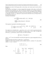
where the objective of eigenvalue preservation is clearly achieved. Investigating the

performance of this new LMI-based reduced order model shows that the new completely
transformed system is better than all the previous reduced models (transformed and non-
transformed). This is clearly shown in Figure 9 where the 3
rd
order reduced model, based on
the LMI optimization transformation, provided a response that is almost the same as the 5
th

order original system response.

0 1 2 3 4 5 6 7 8
-0.02
0
0.02
0.04
0.06
0.08
0.1
0.12
0.14
___ Original, Trans. with LMI, None Trans., Trans. without LMI
Tim e[s]
System Output


Fig. 9. Reduced 3
rd
order models (…. transformed without LMI, non-transformed,
transformed with LMI) output responses to a step input along with the non reduced ( ____
original) system output response. The LMI-transformed curve fits almost exactly on the

original response.
Case #2. For the example of case #2 in subsection 4.1.1, for T
s
= 0.1 sec., 200 input/output
data learning points, and η = 0.0051 with initial weights for the [

d
A
] matrix as follows:

0.0332 0.0682 0.0476 0.0129 0.0439
0.0317 0.0610 0.0575 0.0028 0.0691
0.0745 0.0516 0.0040 0.0234 0.0247
0.0459 0.0231 0.0086 0.0611 0.0154
0.0706
w =
0.0418 0.0633 0.0176 0.0273
⎡
⎤
⎢
⎥
⎢
⎥
⎢
⎥
⎢
⎥
⎢
⎥
⎢

⎥
⎣
⎦


Recent Advances in Robust Control – Novel Approaches and Design Methods

80
the transformed [

A ] was obtained and used to calculate the permutation matrix [P]. The
complete system transformation was then performed and the reduction technique produced
the following 3
rd
order reduced model:
-0.6910 1.3088 -3.8578 -0.7621
( ) -1.3088 -0.6910 -1.5719 ( ) -0.1118 ( )
0 0 -0.3697 0.4466
xt xt ut
⎡⎤⎡⎤
⎢⎥⎢⎥
=+
⎢⎥⎢⎥
⎢⎥⎢⎥
⎣⎦⎣⎦


0.0061 0.0261 0.0111 0.0015
( ) -0.0459 0.0187 -0.0946 ( ) 0.0015 ( )
0.0117 0.0155 -0.0080 0.0014

y
txtut
⎡⎤⎡⎤
⎢⎥⎢⎥
=+
⎢⎥⎢⎥
⎢⎥⎢⎥
⎣⎦⎣⎦

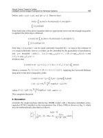
with eigenvalues preserved as desired. Simulating this reduced order model to a step input,
as done previously, provided the response shown in Figure 10.



0 2 4 6 8 10 12 14 16 18 20
-0.02
-0.01
0
0.01
0.02
0.03
0.04
0.05
0.06
0.07
___ Original, Trans. with LMI, None Trans., Trans. without LMI
Time[ s]
System Output

Fig. 10. Reduced 3
rd
order models (…. transformed without LMI, non-transformed,
transformed with LMI) output responses to a step input along with the non reduced (
____ original) system output response. The LMI-transformed curve fits almost exactly on the
original response.
Here, the LMI-reduction-based technique has provided a response that is better than both of
the reduced non-transformed and non-LMI-reduced transformed responses and is almost
identical to the original system response.

Case #3. Investigating the example of case #3 in subsection 4.1.1, for T
s
= 0.1 sec., 200
input/output data points, and η = 1
x 10
-4
with initial weights for [ ]

d
A given as:
Robust Control Using LMI Transformation and Neural-Based Identification for
Regulating Singularly-Perturbed Reduced Order Eigenvalue-Preserved Dynamic Systems

81
0.0048 0.0039 0.0009 0.0089 0.0168
0.0072 0.0024 0.0048 0.0017 0.0040
0.0176 0.0176 0.0136 0.0175 0.0034
0.0055 0.0039 0.0078 0.0076 0.0051
0.01

w =
02 0.0024 0.0091 0.0049 0.0121
⎡
⎤
⎢
⎥
⎢
⎥
⎢
⎥
⎢
⎥
⎢
⎥
⎢
⎥
⎣
⎦

the LMI-based transformation and then order reduction were performed. Simulation results
of the reduced order models and the original system are shown in Figure 11.

0 5 10 15 20 25 30 35 40
-0.2
-0.1
0
0.1
0.2
0.3
0.4

0.5
0.6
0.7
___ Original, Trans. with LMI, None Trans., Trans. without LMI
Time[ s]
System Output

Fig. 11. Reduced 3
rd
order models (…. transformed without LMI, non-transformed,
transformed with LMI) output responses to a step input along with the non reduced (
____ original) system output response. The LMI-transformed curve fits almost exactly on the
original response.
Again, the response of the reduced order model using the complete LMI-based
transformation is the best as compared to the other reduction techniques.

5. The application of closed-loop feedback control on the reduced models
Utilizing the LMI-based reduced system models that were presented in the previous section,
various control techniques – that can be utilized for the robust control of dynamic systems -
are considered in this section to achieve the desired system performance. These control
methods include (a) PID control, (b) state feedback control using (1) pole placement for the
desired eigenvalue locations and (2) linear quadratic regulator (LQR) optimal control, and
(c) output feedback control.
5.1 Proportional–Integral–Derivative (PID) control
A PID controller is a generic control loop feedback mechanism which is widely used in
industrial control systems [7,10,24]. It attempts to correct the error between a measured

Recent Advances in Robust Control – Novel Approaches and Design Methods

82

process variable (output) and a desired set-point (input) by calculating and then providing a
corrective signal that can adjust the process accordingly as shown in Figure 12.





Fig. 12. Closed-loop feedback single-input single-output (SISO) control using a PID
controller.
In the control design process, the three parameters of the PID controller {K
p
, K
i
, K
d
} have to
be calculated for some specific process requirements such as system overshoot and settling
time. It is normal that once they are calculated and implemented, the response of the system
is not actually as desired. Therefore, further tuning of these parameters is needed to provide
the desired control action.
Focusing on one output of the tape-drive machine, the PID controller using the reduced
order model for the desired output was investigated. Hence, the identified reduced 3
rd
order
model is now considered for the output of the tape position at the head which is given as:
original
32
0.0801s 0.133
()
2.1742s 2.2837s 1.0919

Gs
s
+
=
+++

Searching for suitable values of the PID controller parameters, such that the system provides
a faster response settling time and less overshoot, it is found that {K
p
= 100, K
i
= 80, K
d
= 90}
with a controlled system which is given by:
32
controlled
432
7.209s 19.98s 19.71s 10.64
()
s 9.383 22.26s 20.8s 10.64
Gs
s
+++
=
++++

Simulating the new PID-controlled system for a step input provided the results shown in
Figure 13, where the settling time is almost 1.5 sec. while without the controller was greater
than 6 sec. Also as observed, the overshoot has much decreased after using the PID

controller.
On the other hand, the other system outputs can be PID-controlled using the cascading of
current process PID and new tuning-based PIDs for each output. For the PID-controlled
output of the tachometer shaft angle, the controlling scheme would be as shown in Figure
14. As seen in Figure 14, the output of interest (i.e., the 2
nd
output) is controlled as desired
using the PID controller. However, this will affect the other outputs' performance and
therefore a further PID-based tuning operation must be applied.
Robust Control Using LMI Transformation and Neural-Based Identification for
Regulating Singularly-Perturbed Reduced Order Eigenvalue-Preserved Dynamic Systems

83
0 1 2 3 4 5 6 7 8 9 10
0
0.02
0.04
0.06
0.08
0.1
0.12
0.14
Step Response
Time (s ec)
Amplitude

Fig. 13. Reduced 3
rd
order model PID controlled and uncontrolled step responses.

(a) (b)
Fig. 14. Closed-loop feedback single-input multiple-output (SIMO) system with a PID
controller: (a) a generic SIMO diagram, and (b) a detailed SIMO diagram.
As shown in Figure 14, the tuning process is accomplished using G
1T
and G
3T
. For example,
for the 1
st
output:

111 2 11
PID( )
T
YGG RY YGR
=
−== (39)

∴
1
2

PID( )
T
R
G
R-Y
=

(40)
where Y
2
is the Laplace transform of the 2
nd
output. Similarly, G
3T
can be obtained.
5.2 State feedback control
In this section, we will investigate the state feedback control techniques of pole placement
and the LQR optimal control for the enhancement of the system performance.
5.2.1 Pole placement for the state feedback control
For the reduced order model in the system of Equations (37) - (38), a simple pole placement-
based state feedback controller can be designed. For example, assuming that a controller is

Recent Advances in Robust Control – Novel Approaches and Design Methods

84
needed to provide the system with an enhanced system performance by relocating the
eigenvalues, the objective can be achieved using the control input given by:

() () ()
r
ut Kx t rt=− +

(41)
where K is the state feedback gain designed based on the desired system eigenvalues. A
state feedback control for pole placement can be illustrated by the block diagram shown in
Figure 15.

Fig. 15. Block diagram of a state feedback control with {[
or
A
], [
or
B
], [
or
C
], [
or
D
]} overall
reduced order system matrices.

Replacing the control input u(t) in Equations (37) - (38) by the above new control input in
Equation (41) yields the following reduced system equations:

() () [ () ()]
rorrorr
xt Axt B Kxt rt=+−+

 
(42)

() () [ () ()]
or r or r
y
t Cxt D Kxt rt

=
+− +

(43)
which can be re-written as:
() () () ()
rorrorror
xt Axt BKxt Brt=− +

 
() [ ] () ()
rororror
xt A BKxt Brt→=− +



() () () ()
or r or r or
yt C x t D Kx t D rt=− +


() [ ] () ()
or or r or
y
t C DKxt Drt→=− +


where this is illustrated in Figure 16.

Fig. 16. Block diagram of the overall state feedback control for pole placement.

o
r
B
∫
+
+
+
y(t)
u(t)
)(
~
tx
r

)(
~
tx
r
K
-
+
r(t)
o
r
A
o
r
C

or
D
+
KBA
oror
−

∫

+
+
+
y(t)
()
r
xt



()
r
xt


r(t)
or
B
KDC
oror
−

or
D
+
Robust Control Using LMI Transformation and Neural-Based Identification for
Regulating Singularly-Perturbed Reduced Order Eigenvalue-Preserved Dynamic Systems

85
The overall closed-loop system model may then be written as:
() () ()
cl r cl
xt A x t Brt=+


(44)

() () ()
cl r cl
y
tCxtDrt=+

(45)
such that the closed loop system matrix [
A
cl
] will provide the new desired system
eigenvalues.
For example, for the system of case #3, the state feedback was used to re-assign the
eigenvalues with {-1.89, -1.5, -1}. The state feedback control was then found to be of K = [-
1.2098 0.3507 0.0184], which placed the eigenvalues as desired and enhanced the system

performance as shown in Figure 17.

0 10 20 30 40 50 60 70 80 90 100
-0.2
-0.1
0
0.1
0.2
0.3
0.4
0.5
0.6
0.7
Time[s]
System Output

Fig. 17. Reduced 3
rd
order state feedback control (for pole placement) output step response
compared with the original ____ full order system output step response.
5.2.2 Linear-Quadratic Regulator (LQR) optimal control for the state feedback control
Another method for designing a state feedback control for system performance
enhancement may be achieved based on minimizing the cost function given by [10]:

()
0
TT
JxQxuRudt
∞
=+

∫
(46)
which is defined for the system
() () ()xt Axt But
=
+

, where Q and R are weight matrices for
the states and input commands. This is known as the LQR problem, which has received
much of a special attention due to the fact that it can be solved analytically and that the
resulting optimal controller is expressed in an easy-to-implement state feedback control
[7,10]. The feedback control law that minimizes the values of the cost is given by:

() ()ut Kxt
=
− (47)

Recent Advances in Robust Control – Novel Approaches and Design Methods

86
where K is the solution of
1 T
KRBq
−
= and [q] is found by solving the algebraic Riccati
equation which is described by:

1
0
TT

A q qA qBR B q Q
−
+
−+= (48)
where [
Q] is the state weighting matrix and [R] is the input weighting matrix. A direct
solution for the optimal control gain maybe obtained using the MATLAB statement
lqr( , , , )KABQR= , where in our example R = 1, and the [Q] matrix was found using the
output [
C] matrix such as
T
QCC= .
The LQR optimization technique is applied to the reduced 3
rd
order model in case #3 of
subsection 4.1.2 for the system behavior enhancement. The state feedback optimal control
gain was found K = [-0.0967 -0.0192 0.0027], which when simulating the complete system for
a step input, provided the normalized output response (with a normalization factor γ =
1.934) as shown in Figure 18.


0 10 20 30 40 50 60 70 80 90 100
-0.2
-0.1
0
0.1
0.2
0.3
0.4
0.5

0.6
0.7
Time[s]
System Output


Fig. 18. Reduced 3
rd
order LQR state feedback control output step response compared
with the original ____ full order system output step response.
As seen in Figure 18, the optimal state feedback control has enhanced the system
performance, which is basically based on selecting new proper locations for the system
eigenvalues.
5.3 Output feedback control
The output feedback control is another way of controlling the system for certain desired
system performance as shown in Figure 19 where the feedback is directly taken from the
output.
Robust Control Using LMI Transformation and Neural-Based Identification for
Regulating Singularly-Perturbed Reduced Order Eigenvalue-Preserved Dynamic Systems

87

Fig. 19. Block diagram of an output feedback control.

The control input is now given by
() () ()ut Kyt rt=− +
, where
() () ()
or r or
y

tCxtDut=+

. By
applying this control to the considered system, the system equations become [7]:

11
() () [ ( () ()) ()]
() () () ()
[ ] () () ()
[ [ ] ] () [ [ ] ]()
rorrororror
or r or or r or or or
or or or r or or or
or or or or r or or
xt Axt B KCxt Dut rt
Axt BKCxt BKDut Brt
ABKCxtBKDutBrt
ABKIDKCxtBIKD rt
−−
=+− ++
=− − +
=− − +
=− + + +

 



(49)

11
() () [ () ()]
() () ()
[[ ] ] ( ) [[ ] ] ( )
or r or
or r or or
or or r or or
yt C x t D Kyt rt
Cxt DKyt Drt
IDK Cxt IDK Drt
−−
=+−+
=− +
=+ ++



(50)
This leads to the overall block diagram as seen in Figure 20.








Fig. 20. An overall block diagram of an output feedback control.
Considering the reduced 3
rd

order model in case #3 of subsection 4.1.2 for system behavior
enhancement using the output feedback control, the feedback control gain is found to be K =
[0.5799 -2.6276 -11]. The normalized controlled system step response is shown in Figure 21,
where one can observe that the system behavior is enhanced as desired.
o
r
B
∫

+
+
+
y(t)
u(t)
()
r
xt



()
r
xt


K
-
+
r(t)
o

r
A
o
r
C
or
D
+
1
[]
or or or or
A
BKI DK C
−
−+

∫

+
+
+
y(t)
()
r
xt



()
r

xt


r(t)
1
[]
or or
BIKD
−
+
1
[]
or or
IDK C
−
+
oror
DKDI
1
][
−
+
+

Recent Advances in Robust Control – Novel Approaches and Design Methods

88
0 10 20 30 40 50 60 70 80 90 100
-0.2
-0.1

0
0.1
0.2
0.3
0.4
0.5
0.6
0.7
Time[ s]
System Output

Fig. 21. Reduced 3
rd
order output feedback controlled step response compared with the
original ____ full order system uncontrolled output step response.
6. Conclusions and future work
In control engineering, robust control is an area that explicitly deals with uncertainty in its
approach to the design of the system controller. The methods of robust control are designed
to operate properly as long as disturbances or uncertain parameters are within a compact
set, where robust methods aim to accomplish robust performance and/or stability in the
presence of bounded modeling errors. A robust control policy is static - in contrast to the
adaptive (dynamic) control policy - where, rather than adapting to measurements of
variations, the system controller is designed to function assuming that certain variables will
be unknown but, for example, bounded.
This research introduces a new method of hierarchical intelligent robust control for dynamic
systems. In order to implement this control method, the order of the dynamic system was
reduced. This reduction was performed by the implementation of a recurrent supervised
neural network to identify certain elements [
A
c

] of the transformed system matrix [

A ],
while the other elements [
A
r
] and [A
o
] are set based on the system eigenvalues such that [A
r
]
contains the dominant eigenvalues (i.e., slow dynamics) and [
A
o
] contains the non-dominant
eigenvalues (i.e., fast dynamics). To obtain the transformed matrix [

A ], the zero input
response was used in order to obtain output data related to the state dynamics, based only
on the system matrix [
A]. After the transformed system matrix was obtained, the
optimization algorithm of linear matrix inequality was utilized to determine the
permutation matrix [
P], which is required to complete the system transformation matrices
{[

B ], [

C ], [


D ]}. The reduction process was then applied using the singular perturbation
method, which operates on neglecting the faster-dynamics eigenvalues and leaving the
dominant slow-dynamics eigenvalues to control the system. The comparison simulation
results show clearly that modeling and control of the dynamic system using LMI is superior
Robust Control Using LMI Transformation and Neural-Based Identification for
Regulating Singularly-Perturbed Reduced Order Eigenvalue-Preserved Dynamic Systems

89
to that without using LMI. Simple feedback control methods using PID control, state
feedback control utilizing (a) pole assignment and (b) LQR optimal control, and output
feedback control were then implemented to the reduced model to obtain the desired
enhanced response of the full order system.
Future work will involve the application of new control techniques, utilizing the control
hierarchy introduced in this research, such as using fuzzy logic and genetic algorithms.
Future work will also involve the fundamental investigation of achieving model order
reduction for dynamic systems with all eigenvalues being complex.
7. References
[1] A. N. Al-Rabadi, “Artificial Neural Identification and LMI Transformation for Model
Reduction-Based Control of the Buck Switch-Mode Regulator,” American Institute of
Physics (AIP), In: IAENG Transactions on Engineering Technologies, Special Edition of
the International MultiConference of Engineers and Computer Scientists 2009, AIP
Conference Proceedings 1174, Editors: Sio-Iong Ao, Alan Hoi-Shou Chan, Hideki
Katagiri and Li Xu, Vol. 3, pp. 202 – 216, New York, U.S.A., 2009.
[2]
A. N. Al-Rabadi, “Intelligent Control of Singularly-Perturbed Reduced Order
Eigenvalue-Preserved Quantum Computing Systems via Artificial Neural
Identification and Linear Matrix Inequality Transformation,” IAENG Int. Journal of
Computer Science (IJCS), Vol. 37, No. 3, 2010.
[3]
P. Avitabile, J. C. O’Callahan, and J. Milani, “Comparison of System Characteristics

Using Various Model Reduction Techniques,” 7
th
International Model Analysis
Conference, Las Vegas, Nevada, February 1989.
[4]
P. Benner, “Model Reduction at ICIAM'07,” SIAM News, Vol. 40, No. 8, 2007.
[5]
A. Bilbao-Guillerna, M. De La Sen, S. Alonso-Quesada, and A. Ibeas, “Artificial
Intelligence Tools for Discrete Multiestimation Adaptive Control Scheme with
Model Reduction Issues,” Proc. of the International Association of Science and
Technology, Artificial Intelligence and Application, Innsbruck, Austria, 2004.
[6]
S. Boyd, L. El Ghaoui, E. Feron, and V. Balakrishnan, Linear Matrix Inequalities in System
and Control Theory, Society for Industrial and Applied Mathematics (SIAM), 1994.
[7]
W. L. Brogan, Modern Control Theory, 3
rd
Edition, Prentice Hall, 1991.
[8]
T. Bui-Thanh, and K. Willcox, “Model Reduction for Large-Scale CFD Applications
Using the Balanced Proper Orthogonal Decomposition,” 17
th
American Institute of
Aeronautics and Astronautics (AIAA) Computational Fluid Dynamics Conf., Toronto,
Canada, June 2005.
[9]
J. H. Chow, and P. V. Kokotovic, “A Decomposition of Near-Optimal Regulators for
Systems with Slow and Fast Modes,” IEEE Trans. Automatic Control, AC-21, pp. 701-
705, 1976.
[10]

G. F. Franklin, J. D. Powell, and A. Emami-Naeini, Feedback Control of Dynamic Systems,
3
rd
Edition, Addison-Wesley, 1994.
[11]
K. Gallivan, A. Vandendorpe, and P. Van Dooren, “Model Reduction of MIMO System
via Tangential Interpolation,” SIAM Journal of Matrix Analysis and Applications, Vol.
26, No. 2, pp. 328-349, 2004.

Recent Advances in Robust Control – Novel Approaches and Design Methods

90
[12] K. Gallivan, A. Vandendorpe, and P. Van Dooren, “Sylvester Equation and Projection-
Based Model Reduction,” Journal of Computational and Applied Mathematics, 162, pp.
213-229, 2004.
[13]
G. Garsia, J. Dfouz, and J. Benussou, “H
2
Guaranteed Cost Control for Singularly
Perturbed Uncertain Systems,” IEEE Trans. Automatic Control, Vol. 43, pp. 1323-
1329, 1998.
[14]
R. J. Guyan, “Reduction of Stiffness and Mass Matrices,” AIAA Journal, Vol. 6, No. 7,
pp. 1313-1319, 1968.
[15] S. Haykin, Neural Networks: A Comprehensive Foundation, Macmillan Publishing
Company, New York, 1994.
[16]
W. H. Hayt, J. E. Kemmerly, and S. M. Durbin, Engineering Circuit Analysis, McGraw-
Hill, 2007.
[17]

G. Hinton, and R. Salakhutdinov, “Reducing the Dimensionality of Data with Neural
Networks,” Science, pp. 504-507, 2006.
[18]
R. Horn, and C. Johnson, Matrix Analysis, Cambridge University Press, New York, 1985.
[19]
S. H. Javid, “Observing the Slow States of a Singularly Perturbed Systems,” IEEE Trans.
Automatic Control, AC-25, pp. 277-280, 1980.
[20]
H. K. Khalil, “Output Feedback Control of Linear Two-Time-Scale Systems,” IEEE
Trans. Automatic Control, AC-32, pp. 784-792, 1987.
[21]
H. K. Khalil, and P. V. Kokotovic, “Control Strategies for Decision Makers Using
Different Models of the Same System,” IEEE Trans. Automatic Control, AC-23, pp.
289-297, 1978.
[22]
P. Kokotovic, R. O'Malley, and P. Sannuti, “Singular Perturbation and Order Reduction
in Control Theory – An Overview,” Automatica, 12(2), pp. 123-132, 1976.
[23]
C. Meyer, Matrix Analysis and Applied Linear Algebra, Society for Industrial and Applied
Mathematics (SIAM), 2000.
[24]
K. Ogata, Discrete-Time Control Systems, 2
nd
Edition, Prentice Hall, 1995.
[25]
R. Skelton, M. Oliveira, and J. Han, Systems Modeling and Model Reduction, Invited Chapter
of the Handbook of Smart Systems and Materials, Institute of Physics, 2004.
[26]
M. Steinbuch, “Model Reduction for Linear Systems,” 1
st

International MACSI-net
Workshop on Model Reduction, Netherlands, October 2001.
[27]
A. N. Tikhonov, “On the Dependence of the Solution of Differential Equation on a
Small Parameter,” Mat Sbornik (Moscow), 22(64):2, pp. 193-204, 1948.
[28]
R. J. Williams, and D. Zipser, “A Learning Algorithm for Continually Running Fully
Recurrent Neural Networks,” Neural Computation, 1(2), pp. 270-280, 1989.
[29]
J. M. Zurada, Artificial Neural Systems, West Publishing Company, New York, 1992.
5
Neural Control Toward a Unified Intelligent
Control Design Framework for
Nonlinear Systems
Dingguo Chen
1
, Lu Wang
2
, Jiaben Yang
3
and Ronald R. Mohler
4

1
Siemens Energy Inc., Minnetonka, MN 55305
2
Siemens Energy Inc., Houston, TX 77079
3
Tsinghua University, Beijing 100084
4

Oregon State University, OR 97330
1,2,4
USA
3
China
1. Introduction
There have been significant progresses reported in nonlinear adaptive control in the last two
decades or so, partially because of the introduction of neural networks (Polycarpou, 1996;
Chen & Liu, 1994; Lewis, Yesidirek & Liu, 1995; Sanner & Slotine, 1992; Levin & Narendra,
1993; Chen & Yang, 2005). The adaptive control schemes reported intend to design adaptive
neural controllers so that the designed controllers can help achieve the stability of the
resulting systems in case of uncertainties and/or unmodeled system dynamics. It is a typical
assumption that no restriction is imposed on the magnitude of the control signal.
Accompanied with the adaptive control design is usually a reference model which is
assumed to exist, and a parameter estimator. The parameters can be estimated within a pre-
designated bound with appropriate parameter projection. It is noteworthy that these design
approaches are not applicable for many practical systems where there is a restriction on the
control magnitude, or a reference model is not available.
On the other hand, the economics performance index is another important objective for
controller design for many practical control systems. Typical performance indexes include,
for instance, minimum time and minimum fuel. The optimal control theory developed a few
decades ago is applicable to those systems when the system model in question along with a
performance index is available and no uncertainties are involved. It is obvious that these
optimal control design approaches are not applicable for many practical systems where
these systems contain uncertain elements.
Motivated by the fact that many practical systems are concerned with both system stability
and system economics, and encouraged by the promising images presented by theoretical
advances in neural networks (Haykin, 2001; Hopfield & Tank, 1985) and numerous application
results (Nagata, Sekiguchi & Asakawa, 1990; Methaprayoon, Lee, Rasmiddatta, Liao & Ross,
2007; Pandit, Srivastava & Sharma, 2003; Zhou, Chellappa, Vaid & Jenkins, 1998; Chen & York,

2008; Irwin, Warwick & Hunt, 1995; Kawato, Uno & Suzuki, 1988; Liang 1999; Chen & Mohler,
1997; Chen & Mohler, 2003; Chen, Mohler & Chen, 1999), this chapter aims at developing an

Recent Advances in Robust Control – Novel Approaches and Design Methods

92
intelligent control design framework to guide the controller design for uncertain, nonlinear
systems to address the combining challenge arising from the following:
• The designed controller is expected to stabilize the system in the presence of
uncertainties in the parameters of the nonlinear systems in question.
• The designed controller is expected to stabilize the system in the presence of
unmodeled system dynamics uncertainties.
• The designed controller is confined on the magnitude of the control signals.
• The designed controller is expected to achieve the desired control target with minimum
total control effort or minimum time.
The salient features of the proposed control design framework include: (a) achieving nearly
optimal control regardless of parameter uncertainties; (b) no need for a parameter estimator
which is popular in many adaptive control designs; (c) respecting the pre-designated range
for the admissible control.
Several important technical aspects of the proposed intelligent control design framework
will be studied:
• Hierarchical neural networks (Kawato, Uno & Suzuki, 1988; Zakrzewski, Mohler &
Kolodziej, 1994; Chen, 1998; Chen & Mohler, 2000; Chen, Mohler & Chen, 2000; Chen,
Yang & Moher, 2008; Chen, Yang & Mohler, 2006) are utilized; and the role of each tier
of the hierarchy will be discussed and how each tier of the hierarchical neural networks
is constructed will be highlighted.
• The theoretical aspects of using hierarchical neural networks to approximately achieve
optimal, adaptive control of nonlinear, time-varying systems will be studied.
• How the tessellation of the parameter space affects the resulting hierarchical neural
networks will be discussed.

In summary, this chapter attempts to provide a deep understanding of what hierarchical
neural networks do to optimize a desired control performance index when controlling
uncertain nonlinear systems with time-varying properties; make an insightful investigation
of how hierarchical neural networks may be designed to achieve the desired level of control
performance; and create an intelligent control design framework that provides guidance for
analyzing and studying the behaviors of the systems in question, and designing hierarchical
neural networks that work in a coordinated manner to optimally, adaptively control the
systems.
This chapter is organized as follows: Section 2 describes several classes of uncertain
nonlinear systems of interest and mathematical formulations of these problems are
presented. Some conventional assumptions are made to facilitate the analysis of the
problems and the development of the design procedures generic for a large class of
nonlinear uncertain systems. The time optimal control problem and the fuel optimal control
problem are analyzed and an iterative numerical solution process is presented in Section 3.
These are important elements in building a solution approach to address the control
problems studied in this paper which are in turn decomposed into a series of control
problems that do not exhibit parameter uncertainties. This decomposition is vital in the
proposal of the hierarchical neural network based control design. The details of the
hierarchical neural control design methodology are given in Section 4. The synthesis of
hierarchical neural controllers is to achieve (a) near optimal control (which can be time-
optimal or fuel-optimal) of the studied systems with constrained control; (b) adaptive
control of the studied control systems with unknown parameters; (c) robust control of the
studied control systems with the time-varying parameters. In Section 5, theoretical results
Neural Control Toward a Unified
Intelligent Control Design Framework for Nonlinear Systems

93
are developed to justify the fuel-optimal control oriented neural control design procedures
for the time-varying nonlinear systems. Finally, some concluding remarks are made.
2. Problem formulation

As is known, the adaptive control design of nonlinear dynamic systems is still carried out on a
per case-by-case basis, even though there have numerous progresses in the adaptive of linear
dynamic systems. Even with linear systems, the conventional adaptive control schemes have
common drawbacks that include (a) the control usually does not consider the physical control
limitations, and (b) a performance index is difficult to incorporate. This has made the adaptive
control design for nonlinear system even more challenging. With this common understanding,
this Chapter is intended to address the adaptive control design for a class of nonlinear systems
using the neural network based techniques. The systems of interest are linear in both control
and parameters, and feature time-varying, parametric uncertainties, confined control inputs,
and multiple control inputs. These systems are represented by a finite dimensional differential
system linear in control and linear in parameters.
The adaptive control design framework features the following:
• The adaptive, robust control is achieved by hierarchical neural networks.
• The physical control limitations, one of the difficulties that conventional adaptive
control can not handle, are reflected in the admissible control set.
• The performance measures to be incorporated in the adaptive control design, deemed
as a technical challenge for the conventional adaptive control schemes, that will be
considered in this Chapter include:
• Minimum time – resulting in the so-called time-optimal control
• Minimum fuel – resulting in the so-called fuel-optimal control
• Quadratic performance index – resulting in the quadratic performance optimal
control.
Although the control performance indices are different for the above mentioned approaches,
the system characterization and some key assumptions are common.
The system is mathematically represented by

() () ()xax CxpBxu
=
++


(1)
where
n
xG R∈⊆ is the state vector,
l
p
p
R∈Ω ⊂ is the bounded parameter vector,
m
uR∈
is the control vector, which is confined to an admissible control set U ,
[
]
12
() () () ()
n
ax a x a x a x
τ
= "
is an
n
-dimensional vector function of
x
,
11 12 1
21 22 2
12
() ()
() () ()
()

() () ()
l
l
nn nl
CxC x C
Cx Cx Cx
Cx
CxCx Cx
⎡⎤
⎢⎥
⎢⎥
=
⎢⎥
⎢⎥
⎣⎦
is an nl
×
-dimensional matrix function of
x
, and
11 12 1
21 22 2
12
() ()
() () ()
()

() () ()
m

m
nn nm
Bx B x B
Bx Bx B x
Bx
Bx Bx B x
⎡⎤
⎢⎥
⎢⎥
=
⎢⎥
⎢⎥
⎣⎦
is an nm
×
-dimensional matrix function of x .

Recent Advances in Robust Control – Novel Approaches and Design Methods

94
The control objective is to follow a theoretically sound control design methodology to
design the controller such that the system is adaptively controlled with respect to
parametric uncertainties and yet minimizing a desired control performance.
To facilitate the theoretical derivations, several conventional assumptions are made in the
following and applied throughout the Chapter.
AS1: It is assumed that
(.)a
,
(.)C
and

(.)B
have continuous partial derivatives with respect
to the state variables on the region of interest. In other words,
()
i
ax, ()
is
Cx, ()
ik
Bx,
()
i
j
ax
x
∂
∂
,
()
is
j
Cx
x
∂
∂
, and
()
ik
j
Bx

x
∂
∂
for ,1,2,,ij n
=
" ; 1,2, ,km
=
" ; 1,2, ,sl
=
" exist and are continuous
and bounded on the region of interest.
It should be noted that the above conditions imply that
(.)a , (.)C and (.)B satisfy the
Lipschitz condition which in turn implies that there always exists a unique and continuous
solution to the differential equation given an initial condition
00
()xt
ξ
=
and a bounded
control
()ut .
AS2: In practical applications, control effort is usually confined due to the limitation of
design or conditions corresponding to physical constraints. Without loss of generality,
assume that the admissible control set U is characterized by:

{
}
:| | 1, 1, 2, ,
i

Uuu i m=≤="
(2)
where
i
u is u 's i th component.
AS3: It is assumed that the system is controllable.
AS4: Some control performance criteria
J may relate to the initial time
0
t and the final time
f
t . The cost functional reflects the requirement of a particular type of optimal control.
AS5: The target set
f
θ
is defined as
{
}
:(())0
ff
xxt
θψ
=
= where
i
ψ
’s ( 1,2, ,iq
=
" ) are the
components of the continuously differentiable function vector

(.)
ψ
.
Remark 1: As a step of our approach to address the control design for the system (1), the
above same control problem is studied with the only difference that the parameters in Eq.
(1) are given. An optimal solution is sought to the following control problem:
The optimal control problem (
0
P ) consists of the system equation (1) with fixed and known
parameter vector
p
, the initial time
0
t , the variable final time
f
t , the initial state
00
()xxt= ,
together with the assumptions AS1, AS2, AS3, AS4, AS5 satisfied such that the system state
conducts to a pre-specified terminal set
f
θ
at the final time
f
t
while the control
performance index is minimized.
AS6: There do not exist singular solutions to the optimal control problem (
0
P

) as described
in Remark 1 (referenced as the control problem (
0
P ) later on distinct from the original
control problem (
P )).
AS7:
x
p
∂
∂
is bounded on
p
p
∈
Ω and
x
x
∈
Ω .
Neural Control Toward a Unified
Intelligent Control Design Framework for Nonlinear Systems

95
Remark 2: For any continuous function ()
f
x defined on the compact domain
n
x
RΩ⊂ ,

there exists a neural network characterized by
()
f
NN x such that for any positive number
*
f
ε
,
*
|() ()|
ff
fx NN x
ε
−<.
AS8: Let the sufficiently trained neural network be denoted by
(, )
s
NN x
Θ
, and the neural
network with the ideal weights and biases by
*
(, )NN x
Θ
where
s
Θ
and
*
Θ

designate the
parameter vectors comprising weights and biases of the corresponding neural networks.
The approximation of
(, )
f
s
NN x
Θ
to
*
(, )
f
NN x
Θ
is measured by
**
(;;)| (,) (,)|
fs fs f
NN x NN x NN x
δ
ΘΘ = Θ − Θ . Assume that
*
(; ; )
fs
NN x
δ
Θ
Θ is bounded by a
pre-designated number 0,
s

ε
> i.e.,
*
(;;)
s
fs
NN x
δ
ε
Θ
Θ< .
AS9: The total number of switch times for all control components for the studied fuel-
optimal control problem is greater than the number of state variables.
Remark 3: AS9 is true for practical systems to the best knowledge of the authors. The
assumption is made for the convenience of the rigor of the theoretical results developed in
this Chapter.
2.1 Time-optimal control
For the time-optimal control problem, the system characterization, the control objective,
constraints remain the same as for the generic control problem with the exception that the
control performance index reflected in the Assumption AS4 is replaced with the following:
AS4: The control performance criteria is
0
1
f
t
t
Jds=
∫
where
0

t and
f
t are the initial time and the
final time, respectively. The cost functional reflects the requirement of time-optimal control.
2.2 Fuel-optimal control
For the fuel-optimal control problem, the system characterization, the control objective,
constraints remain the same as for the time-optimal control problem with the Assumption
AS4 replaced with the following:
AS4: The control performance criteria is
0
0
1
||
f
t
m
kk
k
t
Je euds
=
⎡
⎤
=+
⎢
⎥
⎣
⎦
∑
∫

where
0
t and
f
t are the
initial time and the final time, respectively, and
k
e ( 0,1,2, ,km
=
" ) are non-negative
constants. The cost functional reflects the requirement of fuel-optimal control as related to
the integration of the absolute control effort of each control variable over time.
2.3 Optimal control with quadratic performance index
For the quadratic performance index based optimal control problem, the system
characterization, the control objective, constraints remain the same with the Assumption
AS4 replaced with the following:
AS4: The control performance criteria is
0
11
(()())()(()()) ( )( )
22
f
t
fffff e e
t
JxtrtStxtrt xQxuuRuuds
τττ
⎡
⎤
=− −+ +−−

⎣
⎦
∫
where
0
t and
f
t
are

Recent Advances in Robust Control – Novel Approaches and Design Methods

96
the initial time and the final time, respectively; and
()0
f
St ≥
,
0Q ≥
, and 0
R ≥ with
appropriate dimensions; and the desired final state ( )
f
rt is the specified as the equilibrium
e
x
, and
e
u
is the equilibrium control.

3. Numerical solution schemes to the optimal control problems
To solve for the optimal control, mathematical derivations are presented below for each of
the above optimal control problems to show that the resulting equations represent the
Hamiltonian system which is usually a coupled two-point boundary-value problem
(TPBVP), and the analytic solution is not available, to our best knowledge. It is worth noting
that in the solution process, the parameter is assumed to be fixed.
3.1 Numerical solution scheme to the time optimal control problem
By assumption AS4, the optimal control performance index can be expressed as
0
0
() 1
f
t
t
Jt dt=
∫

where
0
t is the initial time, and
f
t is the final time.
Define the Hamiltonian function as
(,,) 1 (() () ())
Hxut ax Cx
p
Bxu
τ
λ
=+ + +

where
[]
12 n
τ
λ
λλ λ
= "
is the costate vector.
The final-state constraint is ( ( )) 0
f
xt
ψ
=
as mentioned before.
The state equation can be expressed as
0
() () (),
H
xaxCxpBxutt
λ
∂
=
=+ + ≥
∂


The costate equation can be written as
(() () ())
,
ax Cxp Bxu

H
tT
xx
τ
λλ
∂+ +
∂
−
== ≤
∂∂


The Pontryagin minimum principle is applied in order to derive the optimal control (Lee &
Markus, 1967). That is,
*** * *
(,,,) (,, ,)Hx u t Hx u t
λλ
≤
for all admissible
u .
where
*
u ,
*
x and
*
λ
correspond to the optimal solution.
Consequently,
***

11
() ()
mm
kk kk
kk
Bxu Bxu
ττ
λλ
==
≤
∑∑

Neural Control Toward a Unified
Intelligent Control Design Framework for Nonlinear Systems

97
where ()
k
Bx is the k th column of the ()Bx .
Since the control components
k
u 's are all independent, the minimization of
1
()
m
kk
k
Bxu
τ
λ

=
∑

is equivalent to the minimization of ( )
kk
Bxu
τ
λ
.
The optimal control can be expressed as
**
s
g
n( ( ))
kk
ust=− , where
s
g
n(.)
is the sign function
defined as
s
g
n( ) 1t
=
if 0t > or s
g
n( ) 1t
=
− if 0t

<
; and ( ) ( )
kk
st Bx
τ
λ
= is the k th
component of the switch vector ( ) ( )
St Bx
τ
λ
= .
It is observed that the resulting Hamiltonian system is a coupled two-point boundary-value
problem, and its analytic solution is not available in general.
With assumption AS6 satisfied, it is observed from the derivation of the optimal time control
that the control problem (
0
P
) has bang-bang control solutions.
Consider the following cost functional:
0
2
1
1(())
f
q
t
ii
f
t

i
Jdt xt
ρψ
=
=+
∑
∫

where
i
ρ
's are positive constants, and
i
ψ
's are the components of the defining equation of
the target set
{
}
:(())0
ff
xxt
θψ
=
= to the system state is transferred from a given initial state
by means of proper control, and
q
is the number of components in
ψ
.
It is observed that the system described by Eq. (1) is a nonlinear system but linear in control.

With assumption AS6, the requirements for applying the Switching-Time-Varying-Method
(STVM) are met. The optimal switching-time vector can be obtained by using a gradient-
based method. The convergence of the STVM is guaranteed if there are no singular
solutions.
Note that the cost functional can be rewritten as follows:
0
''
00
[( () (), )]
f
t
t
Jaxbxudt=+<>
∫

where
'
0
1
() 1 2 ,() () ,
q
i
ii
i
ax ax Cxp
x
ψ
ρψ
=
∂

=+ < + >
∂
∑

'
0
1
() 2 [ ] ()
q
i
ii
i
bx Bx
x
τ
ψ
ρψ
=
∂
=
∂
∑
, and ()ax ,
()Cx ,
p
and ()Bx are as given in the control problem (
0
P ).
Define a new state variable
0

()xt
as follows:
''
000
0
() [( () (), )]
t
t
xt ax bxu dt=+<>
∫

Define the augmented state vector
0
xxx
τ
τ
⎡
⎤
=
⎣
⎦
,
'
0
() () (() ())ax a x ax Cxp
τ
τ
⎡
⎤
=+

⎣
⎦
, and
'
0
() () (())Bx b x Bx
τ
τ
⎡⎤
=
⎣⎦
.
The system equation can be rewritten in terms of the augmented state vector as
() ()xax Bxu
=
+

where
00
() 0 ()xt xt
τ
τ
⎡
⎤
=
⎣
⎦
.

Recent Advances in Robust Control – Novel Approaches and Design Methods

98
A Hamiltonian system can be constructed for the above state equation with the costate
equation given by
(() ())ax Bxu
x
τ
λ
λ
∂
=− +
∂

where () |()
ff
J
txt
x
λ
∂
=
∂
.
It has been shown (Moon, 1969; Mohler, 1973; Mohler, 1991) that the number of the optimal
switching times must be finite provided that no singular solutions exist. Let the zeros of
()
k
st− be
,k
j

τ
+
(1,2,,2
k
jN
+
= " ,1,2,,km
=
" ; and
12
,,k
j
k
j
ττ
++
< for
12
12
k
jj N
+
≤<≤ ).
*
,2 1 ,2
1
() [s
g
n( ) s
g

n( )].
k
N
kk
j
k
j
j
ut t t
ττ
+
++
−
=
=−−−
∑

Let the switch vector for the k th component of the control vector be
kk
NN
τ
τ
+
= where
,1
,2
k
k
N
k

kN
τ
ττ τ
+
+
++
⎡⎤
=
⎣⎦
" . Let 2
kk
NN
+
= . Then
k
N
τ
is the switching vector of
k
N
dimensions.
Let the vector of switch functions for the control variable
k
u be defined as
1
2
kk k
k
NN N
N

τ
φφ φ
+
⎡⎤
=
⎢⎥
⎣⎦
" where
1
,
(1) ( )
k
N
j
kk
j
j
s
φτ
−
+
=−
(1,2,,2
k
jN
+
= " ).
The gradient that can be used to update the switching vector
k
N

τ
can be given by
k
N
k
N
J
τ
φ
∇=−

The optimal switching vector can be obtained iteratively by using a gradient-based method.
,1 ,
,
kk k
Ni Ni N
ki
K
τ
τφ
+
=+
where
,ki
K is a properly chosen
kk
NN× -dimensional diagonal matrix with non-negative
entries for the i th iteration of the iterative optimization process; and
,
k

Ni
τ
represents the
i th iteration of the switching vector
k
N
τ
.
Remark 4: The choice of the step sizes as characterized in the matrix
,ki
K must consider two
facts: if the step size is chosen too small, the solution may converge very slowly; if the step
size is chosen too large, the solution may not converge. Instead of using the gradient
descent method, which is relatively slow compared to other alternative such as methods
based on Newton's method and inversion of the Hessian using conjugate gradient
techniques.
When the optimal switching vectors are determined upon convergence, the optimal control
trajectories and the optimal state trajectories are computed. This process will be repeated for
all selected nominal cases until all needed off-line optimal control and state trajectories are
obtained. These trajectories will be used in training the time-optimal control oriented neural
networks.
Neural Control Toward a Unified
Intelligent Control Design Framework for Nonlinear Systems

99
3.2 Numerical solution scheme to the fuel optimal control problem
By assumption AS4, the optimal control performance index can be expressed as
0
00
1

() ||
f
m
t
kk
t
k
Jt e e u dt
=
⎡
⎤
=+
⎢
⎥
⎣
⎦
∑
∫

where
0
t is the initial time, and
f
t is the final time.
Define the Hamiltonian function as
0
1
(,,) | | (() () ())
m
kk

k
Hxut e e u ax Cxp Bxu
τ
λ
=
=+ + + +
∑

where
[
]
12 n
τ
λ
λλ λ
= "
is the costate vector.
The final-state constraint is
(( )) 0
f
xt
ψ
=
as mentioned before.
The state equation can be expressed as
0
() () (),
H
xaxCx
p

Bxut t
λ
∂
=
=+ + ≥
∂


The costate equation can be written as
0
1
(() () ())
(||)
(() () ())
,
m
kk
k
ax Cxp Bxu
H
xx
eeu
ax Cxp Bxu
tT
xx
τ
τ
λλ
λ
=

∂+ +
∂
−= = +
∂∂
∂+
∂+ +
=
≤
∂
∂
∑

The Pontryagin minimum principle is applied in order to derive the optimal control (Lee &
Markus, 1967). That is,
*** * *
(,,,) (,, ,)Hx u t Hx u t
λλ
≤
for all admissible
u
, where
*
u ,
*
x and
*
λ
correspond to the
optimal solution.
Consequently,

** **
11
11
|| ()
|| ()
mm
kk k k
kk
mm
kk k k
kk
eu Bxu
eu Bxu
τ
τ
λ
λ
==
==
+
≤
+
∑
∑
∑∑

where
()
k
Bx is the k th column of the ()Bx .

Since the control components
k
u 's are all independent, the minimization of
11
|| ()
mm
kk k k
kk
eu Bxu
τ
λ
==
+
∑∑
is equivalent to the minimization of | | ( )
kk k k
eu Bxu
τ
λ
+ .
Since
0
k
e ≠
, define ( ) /
kkk
sBxe
τ
λ
= . The fuel-optimal control satisfies the following

condition:
**
**
*
s
g
n( ( )),| ( )| 1
0,| ( )| 1
,| ( ) | 1
kk
kk
k
st st
ust
undefined s t
⎧
−
>
⎪
⎪
=<
⎨
⎪
=
⎪
⎩


Recent Advances in Robust Control – Novel Approaches and Design Methods

100
where
1,2, ,km=
"
.
Note that the above optimal control can be written in a different form as follows:
** *
kk k
uu u
+
−
=+
where
**
1
s
g
n( ( ) 1) 1
2
kk
ust
+
⎡⎤
=−−+
⎣⎦
, and
**
1
s
g

n( ( ) 1) 1
2
kk
ust
−
⎡⎤
=
−+−
⎣⎦
.
It is observed that the resulting Hamiltonian system is a coupled two-point boundary-value
problem, and its analytic solution is not available in general.
With assumption AS6 satisfied, it is observed from the derivation of the optimal fuel control
that the control problem (
0
P
) only has bang-off-bang control solutions.
Consider the following cost functional:
0
2
0
11
|| (())
f
q
m
t
kk ii
f
t

ki
Jeeudt xt
ρψ
==
⎡⎤
=+ +
⎢⎥
⎣⎦
∑∑
∫

where
i
ρ
's are positive constants, and
i
ψ
's are the components of the defining equation of
the target set
{
}
:(())0
ff
xxt
θψ
=
=
to the system state is transferred from a given initial state
by means of proper control, and q is the number of components in
ψ

.
It is observed that the system described by Eq. (1) is a nonlinear system but linear in control.
With assumption AS6, the requirements for the STVM's application are met. The optimal
switching-time vector can be obtained by using a gradient-based method. The convergence
of the STVM is guaranteed if there are no singular solutions.
Note that the cost functional can be rewritten as follows:
0
''
00
1
[( () (), ) | |]
f
m
t
kk
t
k
Jaxbxu eudt
=
=+<>+
∑
∫

where
'
00
1
() 2 ,() () ,
q
i

ii
i
ax e ax Cxp
x
ψ
ρψ
=
∂
=+ < + >
∂
∑

'
0
1
() 2 [ ] ()
q
i
ii
i
bx Bx
x
τ
ψ
ρψ
=
∂
=
∂
∑

, and ()ax ,
()Cx
,
p
and
()Bx
are as given in the control problem (
0
P
).
Define a new state variable
0
()xt as follows:
''
000
0
1
() [( () (), ) | |]
m
t
kk
t
k
xt ax bxu e u dt
=
=+<>+
∑
∫

Define the augmented state vector

0
xxx
τ
τ
⎡
⎤
=
⎣
⎦
,
'
0
() () (() ())ax a x ax Cxp
τ
τ
⎡
⎤
=+
⎣
⎦
, and
'
0
() () (())Bx b x Bx
τ
τ
⎡
⎤
=
⎣

⎦
.
The system equation can be rewritten in terms of the augmented state vector as
() ()xax Bxu=+

where
00
() 0 ()xt xt
τ
τ
⎡
⎤
=
⎣
⎦
.
Neural Control Toward a Unified
Intelligent Control Design Framework for Nonlinear Systems

101
The adjoint state equation can be written as
(() ())ax Bxu
x
τ
λ
λ
∂
=− +
∂


where () |()
ff
J
txt
x
λ
∂
=
∂
.
It has been shown (Moon, 1969; Mohler, 1973; Mohler, 1991) that the number of the optimal
switching times must be finite provided that no singular solutions exist. Let the zeros of
() 1
k
st−− be
,k
j
τ
+
(1,2,,2
k
jN
+
= " ,1,2,,km
=
" ; and
12
,,k
j
k

j
ττ
++
< for
12
12
k
jj N
+
≤<≤ ) which
represent the switching times corresponding to positive control
*
k
u
+
, the zeros of ( ) 1
k
st−+
be
,k
j
τ
−
(
1,2, ,2
k
jN
−
= "
,

1,2, ,km
=
"
; and
12
,,k
j
k
j
ττ
−−
< for
12
12
k
jj N
−
≤<≤
) which represent
the switching times corresponding to negative control
*
k
u
−
. Altogether
,k
j
τ
+
's and

,k
j
τ
−
's
represent the switching times which uniquely determine
*
k
u
as follows:
*
,2 1 ,2
1
,2 1 ,2
1
1
() { [s
g
n( ) s
g
n( )]
2
[sgn( ) sgn( )]}.
k
k
N
kkjkj
j
N
kj kj

j
ut t t
tt
ττ
ττ
+
−
++
−
=
−−
−
=
=
−−−−
−−−
∑
∑

Let the switch vector for the k th component of the control vector be
()()
kk k
NN N
τ
ττ
ττ τ
+−
⎡⎤
=
⎢⎥

⎣⎦
where
,1
,2
k
k
N
k
kN
τ
ττ τ
+
+
++
⎡
⎤
=
⎣
⎦
" and
,1
,2
k
k
N
k
kN
τ
ττ τ
−

−
−−
⎡
⎤
=
⎣
⎦
" . Let
22
kkk
NNN
+−
=+. Then
k
N
τ
is the switching vector of
k
N dimensions.
Let the vector of switch functions for the control variable
k
u be defined as
1
221 22
kk kk k
kk kk
NN NN N
NN NN
φφ φφ φ
++ +−

++
⎡⎤
=
⎢⎥
⎣⎦
"" where
1
,
(1) ( ( ) 1)
k
N
j
kkkj
j
es
φτ
−
+
=
−+
(1,2,,2
k
jN
+
= " ), and
,
2
(1) ( ( ) 1)
k
k

N
j
kkkj
jN
es
φτ
+
−
+
=
−− (1,2,,2
k
jN
−
= " ).
The gradient that can be used to update the switching vector
k
N
τ
can be given by
k
N
k
N
J
τ
φ
∇=−

The optimal switching vector can be obtained iteratively by using a gradient-based method.

,1 ,
,
kk k
Ni Ni N
ki
K
τ
τφ
+
=+
where
,ki
K is a properly chosen
kk
NN× -dimensional diagonal matrix with non-negative
entries for the i th iteration of the iterative optimization process; and
,
k
Ni
τ
represents the
i th iteration of the switching vector
k
N
τ
.
When the optimal switching vectors are determined upon convergence, the optimal control
trajectories and the optimal state trajectories are computed. This process will be repeated for

Recent Advances in Robust Control – Novel Approaches and Design Methods

102
all selected nominal cases until all needed off-line optimal control and state trajectories are
obtained. These trajectories will be used in training the fuel-optimal control oriented neural
networks.
3.3 Numerical solution scheme to the quadratic optimal control problem
The Hamiltonian function can be defined as
1
(,,) ( ( ) ( )) ( )
2
ee
Hxut xQx u u Ru u a Cp Bu
ττ τ
λ
=+−−+++

The state equation is given by
H
xaCpBu
λ
∂
==++
∂


The costate equation can be given by
()aCpBu
H
Qx
xx

τ
λλ
∂+ +
∂
−= = +
∂∂


The stationarity equation gives
()
0()
e
aCpBu
H
Ru u
uu
τ
λ
∂+ +
∂
== +−
∂∂

u can be solved out as
1
e
uRB u
τ
λ
−

=
−+
The Hamiltonian system becomes
1
1
() () ()( )
( ( ) ( ) ( )( ))
e
e
xax CxpBx RB u
ax Cxp Bx R B u
Qx
x
τ
ττ
λ
λ
λλ
−
−
⎧
=+ + − +
⎪
⎨
∂+ + − +
−= +
⎪
∂
⎩




Furthermore, the boundary condition can be given by
() ()(() ())
ffff
tStxtrt
λ
=
−

Notice that for the Hamiltonian system which is composed of the state and costate
equations, the initial condition is given for the state equation, and the constraints on the
costate variables at the final time for the costate equation.
It is observed that the Hamiltonian system is a set of nonlinear ordinary differential
equations in
()xt and ()t
λ
which develop forward and back in time, respectively. Generally,
it is not possible to obtain the analytic closed-form solution to such a two-point boundary-
value problem (TPBVP). Numerical methods have to be employed to solve for the
Hamiltonian system. One simple method, called shooting method may be used. There are
other methods like the “shooting to a fixed point” method, and relaxation methods, etc.
Neural Control Toward a Unified
Intelligent Control Design Framework for Nonlinear Systems

103
The idea for the shooting method is as follows:
1.
First make a guess for the initial values for the costate.
2.

Integrate the Hamiltonian system forward.
3.
Evaluate the mismatch on the final constraints.
4.
Find the sensitivity Jacobian for the final state and costate with respect to the initial
costate value.
5.
Using the Newton-Raphson method to determine the change on the initial costate
value.
6.
Repeat the loop of steps 2 through 5 until the mismatch is close enough to zero.
4. Unified hierarchical neural control design framework
Keeping in mind that the discussions and analyses made in Section 3 are focused on the
system with a fixed parameter vector, which is the control problem (
0
P
). To address the
original control problem (
P
), the parameter vector space is tessellated into a number of sub-
regions. Each sub-region is identified with a set of vertexes. For each of the vertexes, a
different control problem (
0
P
) is formed. The family of control problems (
0
P
) are combined
together to represent an approximately accurate characterization of the dynamic system
behaviours exhibited by the nonlinear systems in the control problem (

P
). This is an
important step toward the hierarchical neural control design framework that is proposed to
address the optimal control of uncertain nonlinear systems.
4.1 Three-layer approach
While the control problem ( P ) is approximately equivalent to the family of control
problems (
0
P ), the solutions to the respective control problems (
0
P ) must be properly
coordinated in order to provide a consistent solution to the original control problem (
P ).
The requirement of consistent coordination of individual solutions may be mapped to the
hierarchical neural network control design framework proposed in this Chapter that
features the following:
•
For a fixed parameter vector, the control solution characterized by a set of optimal state
and control trajectories shall be approximated by a neural network, which may be
called a nominal neural network for this nominal case. For each nominal case, a
nominal neural network is needed. All the nominal neural network controllers
constitute the nominal layer of neural network controllers.
•
For each sub-region, regional coordinating neural network controllers are needed to
coordinate the responses from individual nominal neural network controllers for the
sub-region. All the regional coordinating neural network controllers constitute the
regional layer of neural network controllers.
•
For an unknown parameter vector, global coordinating neural network controllers are
needed to coordinate the responses from regional coordinating neural network

controllers. All the global coordinating neural network controllers constitute the global
layer of neural networks controllers.
The proposed hierarchical neural network control design framework is a systematic
extension and a comprehensive enhancement of the previous endeavours (Chen, 1998; Chen
& Mohler & Chen, 2000).