Emerging Communications for Wireless Sensor Networks Part 2 ppt

Wireless Sensor Networks Applications via High Altitude Systems

13

2
X

Wireless Sensor Networks Applications
via High Altitude Systems
Zhe Yang and Abbas Mohammed

Blekinge Institute of Technology
Sweden

1. Introduction
Wireless sensor networking is a fast emerging subfield in the field of wireless networking.
It is a key technology for the future ad has been identified as one of the most important
technologies for this century (Akyildiz et al., 2002; Business Week, 1999; Technology Review,
2003). These sensors are generally equipped with data processing, communication, and
information collecting capabilities. They can detect the variation of ambient conditions in
the environment surrounding the sensors and transform them into electric signal (e.g.,
temperature, sound, image). Interests in sensor networks have motivated intensive research
in the past few years emphasizing the potential of collaboration among sensors in data
collecting and processing, coordination and management of the sensing activity and date
flow to the sink.
Depending on application to reveal some characteristics about phenomena in the area,
sensor nodes can be deployed on the ground, in the air, under water, on bodies, in vehicles
and inside buildings (Akyildiz et al., 2002). Thus, these connected sensor nodes have many
promising applications in many fields (e.g., consumer, military, health, environment,
security). Deployment of these sensor nodes can be in random fashion like dropping from a
helicopter (a disaster management setup), or manual (deploying nodes in a building to

detect the movement of human) (Akyildiz et al., 2002).
Sensor nodes are usually constrained in energy and bandwidth (Akyildiz et al., 2002). Such
constraints combined with the deployment of a large number of sensor nodes are challenges
to the design and maintenance of sensor networks. Energy-awareness has to be considered
at all layers of networking protocol stack. It is also related to physical and link layers which
are generally common for all kind of sensor applications. Research on these layers has been
focused on radio communication hardware, energy-aware media access control (MAC)
protocols (Demirkol et al., 2006; Hill et al., 2000; Intel, 2004; Jiang et al., 2006). The main aim
at the network layer is to find ways for energy-efficient and reliable route setup from sensor
nodes to the sink in order to maximally extend the lifetime of network.
HAPs are either aircraft or airships operating at an altitude of 17 km above the ground.
They have been suggested by the International Telecommunication Union (ITU) for
providing communications in mm-wave broadband wireless access (BWA) and the third
generation (3G) communication frequency bands (Elabdin et al., 2006; Thornton et al., 2003;


14

Emerging Communications for Wireless Sensor Networks

Tozer & Grace, 2001). Currently, investigations on HAPs have been carried on in the 3G
telecommunication and broadband wireless services. These platforms are regarded to be based
on lighter-than-air vehicles or conventional aircraft proposed at various stages of development
(Tozer & Grace, 2001). Employing unpiloted, solar-powered platforms in different altitudes can
ultimately make the systems more reliable and competitive in the future.
HAP systems have many characteristics to make it competitive to be adopted in different
telecommunication and wireless communication applications, e.g. a mobile sink in WSN.
HAPs can provide high receiver elevation angle, line of sight (LOS) transmission, large
coverage area and mobile deployment etc. The system combines the advantages of
terrestrial and satellite systems, and furthermore contributes to a better overall system

performance, greater system capacity and cost-effective deployment (Mohammed et al.,
2008). Many countries have made significant efforts in the research of HAP systems and
their potential applications. A company StratXX® in Switzerland has started to develop
three different platforms operating from 3 km to 17 km above the ground to provide various
services, e.g. mobile multimedia transmission, local navigation and remote sensing (StratXX,
2008). A similar scenario of using unmanned autonomous vehicle (UAV) to transfer
information in the distributed wireless sensor system has been proposed (Vincent et al., 2006)
and shown to be an energy-efficient solution.
In this chapter, we explore and analyze the potential of using HAPs in WSN applications to
establish a HAP-WSN system. The HAP-WSN system is composed of a large number of
sensor nodes, which can monitor and collect information about the physical environment
and transmit the data to another location for processing in an ad-hoc manner, and a HAP,
which collects information from sensor nodes as a remote sink above the ground. Reliable
communication links are analyzed between sensor nodes and HAPs to achieve LOS in most
cases based on the height of the platform. The HAP-WSN can be deployed in inaccessible or
disaster environments, where sensor nodes and HAPs are both powered by battery, which
means energy consumption is the key concept in the system design. The chapter is
organized as follows: in section 2, an introduction to WSN and HAP-WSN system is given.
Two scenarios of HAP-WSN are proposed based on the cell formation of the HAP system
and sensor node radio link. In section 3, the configuration and simulation results in the
system level of HAP-WSN are presented. In section 4, the configuration and simulation
results in the physical layer are presented. In section 5, conclusions and future research are
given.

2. High Altitude Platform-Wireless Sensor Network System
2.1 WSN communication scenarios and design issues
A typical sensor network contains a large number of sensor nodes with data processing and
communication capabilities. The sensor nodes send collected data via radio transmitter, to a
sink either directly or through other nodes in a multi-hop fashion. The technological
advances in this field result in the decrease of the size and cost of sensors and enabled the

development of smart disposable micro sensors, which can be networked through wireless
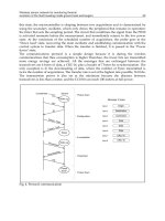
links. Fig. 1 shows the communication architecture of a WSN. Sensor nodes organize
themselves to collect highly reliable information about the phenomenon, and route data via
other sensors to the sink. The sink in Fig. 1 could be either a fixed or mobile node with the


Wireless Sensor Networks Applications via High Altitude Systems

15

capability of connecting sensor networks to the outer existing communication infrastructure,
e.g. internet, cellular and satellite networks.
Internet or  
Satellite

User Task Management

SINK

Sensor nodes

Fig. 1. General communication scenarios of a WSN
Due to the number of sensor nodes and the dynamics of their operating environment, it
poses unique challenges in the design of sensor network architecture.
Dynamic network: Basically a WSN consists of three components: sensor node, sink and
event. Sensor nodes and sink are assumed to be fixed and mobile. Although currently
sensor nodes in most applications are assumed to be stationary, it is still necessary to
support the mobility of sinks or gateway in the network. Thus the stability of data
transferring is an important design factor, in addition to energy, bandwidth etc (Akyildiz et
al., 2002). Moreover the phenomenon could also be dynamic, which requires periodic report

to the sink.

Energy constrains: The process of data routing in the network is greatly affected by
energy considerations, routing path and radio link. Since the radio transmission in
practical scenarios degrades with distance much faster than transmission in free
space, means that communication distance and energy must be well managed
(Chong & Kumar, 2003). Directed routing would perform well enough if all the
sensor nodes are close to the sink. However, most of the time, it is necessary to use
multi-hop routing to consume less power than directed routing, since sensors are
randomly scattered in the area.

Propagation environment: Sensor nodes are deployed on the ground which leads
to a relative low height of antenna on a sensor node and a small distance to the
radio horizon. Non line of sight (NLOS) signal transmission in WSN is
predominant in most directions since the complicated environment of deployment
can cause severe attenuations. Signal power at a distance d away from the
transmitter may be estimated as 1/dn, where n=2 for propagation in free space, but
n is between 2 and 4 for low lying antenna deployments in practical WSNs
(Vincent et al., 2006).
There are other issues such as coverage area, scalability, transmission media, routing
protocols, which could also affect the design and performance of the network (Akyildiz et
al., 2002; Chong & Kumar, 2003). All the solutions to these issues need to reduce the energyconsumption and prolong the lifetime of WSN in most applications.
2.2 HAP-WSN System Scenarios and Advantages
Current research in HAPs has widely adopted two proposed types of cell planning in HAP
system. By subdividing the coverage area of the HAP into one or multiple cells, the HAP


16

Emerging Communications for Wireless Sensor Networks

antenna payload has potential to provide a high gain in each cell planning scenario. In
(Thornton et al., 2003; Yang et al., 2007), the coverage area has been divided into 121 and 19
cells in order to improve the capacity of HAP system. Based on the architecture of HAPs
and WSN, we propose two configurations for HAP-WSN systems for different applications.
The first scenario is shown in Fig. 2. The sensor nodes inside the HAP cells are transmitting
information directly to the HAP. The main aim of the scenario is to reduce the complexity
and remove energy-consumption of multi-hop transmissions in WSN. It is suitable for WSN
applications with low data transmission in large coverage area.
HAP

Internet /
Satellite
network

Signal from sensor

R

HAP coverage area radius
sensor node

R
User Task Management

R

HAP coverage area

Fig. 2. A HAP-WSN system in a single cell configuration.

Fig. 3 shows the second system configuration of the HAP-WSN. The sensor nodes inside the
HAP cell are organized into a cluster, where one node with the higher-energy is selected as
the cluster head. Senor nodes as cluster members collect information and send to the cluster
head, which is responsible to send all data to the HAP. The cluster formation in WSNs is
typically based on the energy reserve of sensors and their distances to the cluster head
(Akyildiz et al., 2002). The main aim of the scenario is to reduce the complexity of a multihop WSN and maintain the energy consumption of all sensor nodes. It can be employed in
WSN applications with high data transmission requirement, e.g. multimedia.
Signal from sensor

HAP
Internet /
Satellite
network

R

HAP coverage area radius
sensor node (cluster member)
sensor node (cluster head)

R
User Task Management

Fig. 3. A HAP-WSN system in a multi-cell configuration
The HAP-WSN system has advantages of HAP system which is employed as a sink in the
WSN:

Reducing complexity of multi-hop transmission and achieving energy-efficiency: A
multi-hop routing has been under investigations because the radio link is usually
constrained by obstructions on the ground. HAPs are often considered to be

located a few kilometers above the ground, where it can establish a LOS link


Wireless Sensor Networks Applications via High Altitude Systems



17

between the sensor node and the HAP sink. Therefore HAPs offer a potential of
reducing or removing transmission burden in WSN, organize communications
based multiple access schemes, e.g. TDMA, CDMA, to reduce energy consumption
in sensor nodes.
Low cost and rapid mobile deployment: It is believed that the cost of HAP is
considerably cheaper than that of a satellite because HAPs do not require
expensive launch and maintenance (Tozer & Grace, 2001). The HAP as a sink, can
be reused, repaired and replaced quickly for applications of WSNs, e.g. disaster
and emergency surveillance where it has clear advantages. It may stay in the sky
for a long period, which can prolong the life of the WSN.

3. System Level Configuration and Simulation Performance
3.1 HAP system antenna and propagation issues
In this work we employ a directive antenna payload on HAPs, which can ensure more
power radiated in the desired directions. The HAP antenna payload is assumed to be
composed of either a single or multiple antennas according to the cell formation. The
antenna radiation model is presented in (Thornton et al., 2003). The gain of the antenna of
HAP AH (), at an angle  with respect to its boresight, is approximated by a cosine function
raised to a power roll-off factor n and a notional flat sidelobe level Sf. GH represents the
boresight gain of the HAP antenna.
AH ( )  G H (max[cos( ) nH , s f ])

(1)
The antenna peak gain is accordingly achieved at the centre of the HAP cell. The HAP
antenna beamwidth is initially defined by its 10dB set to be equal to the subtended angle
away from the antenna boresight of the central cell to the edge of the HAP coverage area or
the central HAP cell corresponding to the single and multi-cell formations. After defining
the beamwidth, the boresight gain is calculated as (Thornton et al., 2003):

Gboresight 

32 ln 2
2 2 3dB

(2)

We select the roll-off factor n to let the radiation curve falling to 10 dB lower than the
maximum value. Fig. 4 shows the two HAP antenna radiation masks corresponding to the
single or multiple cell structures in the system.


18

Emerging Communications for Wireless Sensor Networks

Fig. 4. HAP antenna radiation masks in a single cell and multi-cell formation.
Distance attenuation is the empirically observed long-term trend in signal loss as a function
distance, which is typically proportional to the range raised to some power. A shadowing
fading is used to represent the shadowing effect, which considers the surrounding
environmental clutter that may be different at two locations with the same separation
distance. In our scenario, the pathloss between HAP and sensor node is expressed as the
log-distance pathloss and log-normal shadowing model:

PL ( d )[ dB ]  PL ( d 0 )[ dB ]  10 n log(

d
)  X
d0

(3)

where n is the pathloss exponent, d0 is the reference distance and d is the separation distance
between HAP and sensor node. The value of n is between 2 and 6 depending on the
propagation environment. X denotes a zero mean Gaussian random variable with a
standard deviation  (in dB). The model shows that the pathloss at the particular location is
random and log-normally distributed about the mean distance dependent value.
3.2 System evaluation criteria and parameters
Considering a sensor node in the location (x,y) to communicate with the HAP, performance
can be evaluated by energy bit to noise spectral density ratio in (4):

Eb
P A A PL SH
( x, y )  s s H
N0
N 0 Rb

(4)

where,
Ps is the transmission power of a sensor node in the target HAP cell.
As and Au are antenna gains of a sensor node and HAP respectively.
PLSH is the signal pathloss due to distance attenuation and shadowing effect depending on

the location of sensor node.


Wireless Sensor Networks Applications via High Altitude Systems

19

Rb is the data rate of senor node.
N0 is the noise power spectral density.
Evaluation parameters are shown in Table 1. The physical later (PHY) parameters, e.g. data
rate, sensor node transmit power, are referred to product data sheets of the company
Crossbow® specializing on the sensor network technology (Crossbow, 2008). Parameters of
the low speed (Rb=38.4 kbps) and high speed (Rb=250 kbps) senor nodes are referred for
different applications.
Parameters
Data Rate (Rb)
Tx Power (Ps)
Tx Antenna Gain Rx (As)

Settings
250 kbps / 38.4 kbps
3 dBm / 5 dBm
1

HAP Antenna Boresight (GH)
HAP Height
Coverage Radius (R)
Cell Radius
Pathloss Exponent (n)
Propagation Model

Shadowing Std. Deviation ( )
ISM Frequency Band
Noise Power Spectral Density (N0)

7 dB / 16 dB
17 km (typical)
30 km (typical)
30 km/8km (multi-cell)
2
Free space
2 dB (Log-normal)
2.4 GHz /868 MHz
3.98e-21 W/Hz

Table 1. System level simulation parameters

3.3 System level evaluation results
The cumulative distribution function (CDF) of Eb/N0 is used to evaluate the system
performance. Fig. 5 shows the CDF of Eb/N0 of the received signal in single cell and multi
cell scenario with different transmission rate. According to the product data sheet in
(Crossbow, 2008), industrial-scientific-medical (ISM) band at 868 MHz and 2.4 GHz is
selected, respectively. It can be seen that transmission from sensor node to HAP at 17 km in
two scenarios is possible under the coverage area of 30 km in radius. The performance of
sensors in multi cell scenario is enhanced compared to the single cell HAP-WSN system
with the same transmission rate due to improved HAP cellular antenna radiation profile.

Fig. 5. Eb/N0 of sensor node with different transmission rate in the single cell and multi cell
HAP-WSN scenario

20

Emerging Communications for Wireless Sensor Networks

4. Physical Layer Configuration and Simulation
Reliable communication links are needed to be established between sensor nodes and HAPs
to achieve a LOS in most cases based on the height of the platform. Our investigations in
section 3 show the possibility of establishing a radio link between HAPs and sensor nodes.
In this section, we investigate the performance of the promising multiple access scheme
based on OFDM in conjunction with the HAP served as a mobile sink to communicate with
multiple sensor nodes.
4.1 Time-varying HAP channel characteristics
The HAP communications channel exhibits time-varying characteristics due to the motion of
the platform or receivers and frequency selectivity due to the multipath propagation.
Doppler spectrum can be used to characterize a fading channel and determine if the fading
is fast or slow. A simpler parameter, the maximum Doppler spread fm, can be used to
determine the channel coherence time Tc as (Rappaport, 1996):

Tc 

9
16f m

(5)

where the maximum Doppler spread fm at the carrier frequency fo is:

f m  f d ,HAP  f d ,sensor  [v HAP  v sensor ]

f0

c

(6)

where vHAP and vsensor is the speed of HAP and sensor node, respectively. According to
(Papathanassiou et al., 2001), the Doppler shift exhibits a well-behaved and rather
deterministic variation with time. If we assume the HAP station is not moving, the
multipath signals arriving at the HAP demonstrate unequal but relative small Doppler shifts,
which illustrates that the second Doppler spread component exhibits a relatively small value
and can be modeled in accordance to the typical techniques employed in terrestrial mobile
radio system (Palma-Lazgare & Delgado-Penin, 2006; Papathanassiou et al., 2001).
In HAP-WSN applications, sensor nodes are mostly not capable of mobility and thus we
don’t take account of the movement of sensor nodes. It is one of advantages of using aerial
platform compared to UAV since platforms can be more stably deployed upon the area of
interest with a long duration.
The selectivity of channel is evaluated by the coherence bandwidth Bc of the channel, where
Bc is approximately equal to the inverse of the maximum delay spread m. In time domain, if
the bandwidth of a signal is larger than the reciprocal of the maximum delay spread m, each
multipath signal can be modelled separately since different paths are resolvable. For a
typical LEO channel, the m ranges from 250 to 800 ns (Papathanassiou et al., 2001). Due to
similarities of HAP and LEO satellites, we model the HAP channel as a slow-varying and
frequency-selective fading channel. We assume the HAP is relatively stationary, thus the
Doppler shift due to the motion of the HAP is assumed to be eliminated. The channel is


Wireless Sensor Networks Applications via High Altitude Systems

21

regarded to be a quasi-stationary, and so the fading profile can be regarded to be invariant

during the period of one symbol.
The HAP channel is modelled as an impulse channel response h(t) with a sequence of
discrete-time complex valued components. This sequence of discrete-time complex valued
taps of a channel can be generally expressed by the vector h, which is equal to [h1h2…hl],
where l is the length of discrete-time channel length, and hl is the complex value of the lth tap.
HAP channel modelling parameters are listed in Table 2.
HAP Speed (vHAP)
Node Speed (vsensor)
System bandwidth (B)
Carrier Frequency
Channel Model
Max delay spread (m)

stationary
stationary
5 MHz
ISM band 2.4GHz
Time-Flat
Frequency-Selective
500 ns

Power delay profile

exponential with m

Fading

Ricean
Rayleigh

Table 2. HAP channel characteristics

4.2 Multiple access schemes of OFDM
Orthogonal frequency-division multiplexing/Time division multiple access (OFDM/TDMA)
is based on OFDM transmission scheme and time-division multiple access. Usually the
overall bandwidth in OFDM/TDMA is divided into N subcarriers, and each subcarrier is
carrying relatively small signalling rate. It has to be noticed that a precise synchronization
between sensor nodes and HAP is required in order to have the flexibility and multiple
node accessing. Furthermore the situation leads to a high implementation complexity both
in sensor nodes and HAP. In this chapter, we consider a light version of OFDM/TDMA,
where a single sensor node uses a full time slot to transmit, and the data rate stream is split
into a number of low rate signals modulated in each subcarrier.
Consider the equation for the baseband complex signal of one OFDM symbol in the discretetime domain:
N 1

x data ( n )   X k exp( j
k 0

2
kn )
N

n  (0, 1,2,  , N - 1)

(7)

We use N-long vector Xdata to denote the total OFDM data to be part of the IFFT output:

X data  xdata ,1 , xdata , 2 ,..., x data , N 

(8)

Furthermore, let XGI be an NGI-long vector expressing the guard interval (GI) precursor
signal of Xdata. XGI is chosen to be equal the last NGI elements of Xdata, and is denoted as
cyclic prefix (CP). So a completed transmitted OFDM symbol is given by:


22

Emerging Communications for Wireless Sensor Networks

X  X GI X data 

(9)

Adjacent orthogonal subcarrier frequency separation Bsub is equal to B/N, and is chosen to let
each subcarrier experience a favourable frequency non-selective fading based on N. Usually
N is chosen to make the minimum coherence bandwidth Bc, which is approximately equal to
the inverse of the maximum delay spread m, 10 times higher than the Bsub (Papathanassiou
et al., 2001).

Bsub  ( B / N ) 

Bc
1

10 10 m

(10)

4.3 Simulation setup and results
For a HAP channel at a carrier frequency of 2.4 GHz with m equal to 500 ns, the minimum
coherence bandwidth is equal to 2 MHz. Therefore, if we choose N equal to 64, the
bandwidth of an individual carrier frequency is equal to 78.125 kHz. Each subcarrier can be
guaranteed to be nonselective. In order to keep the orthogonality of the OFDM symbol, CP
is inserted and the NGI is equal to 3. Therefore, the duration of CP is equal to 0.6 ms, which
is larger than the m. In an individual OFDM symbol, CP occupies 4.4 percentage of the
symbol X and can be regarded to be high-efficient transmission. The channel estimation is
performed base on pilot symbols with a data interval at 8 in one OFDM symbol (Cai &
Giannakis, 2004). In order to reduce the complexity of the problem, we have adopted a
simplified but valuable approach purely based on BER performance, which can be achieved
by a single sensor node. In other words, multiple sensor transmission scenario is not
considered in our simulations since it usually requires a precise synchronization when a
large number of sensor nodes transmitting at the same time. No coding schemes are
considered in the simulation. Binary phase-shift keying (BPSK) is used to modulate sensor
node data rate Rb at 250 kbps. The system is assumed to be perfectly synchronized.

Fig. 6. BER performance of OFDM/TDMA in HAP-WSN


Wireless Sensor Networks Applications via High Altitude Systems

23

Simulation results in Fig. 6 show the bit error rate (BER) for N at 64. Generally, multipath
can degrade the system performance due to severe signal attenuation. However, one of the
main advantages of OFDM scheme is its improved performance and robustness in
multipath environments, which is predominant in signal transmission of WSN.
Consequently, it can be seen from Fig. 6 that there is a little difference in the BER
performance under Rayleigh and Ricean fading in the investigated scenario.

5. Conclusion and Future Research
In this chapter, we have shown the scenarios of using HAP as a sink in the WSN in ISM
band for different data rate transmission and examined the performance in the system level
and physical layer. The HAP-WSN system can reduce complexity of the WSN and prolong
the lifetime of sensor node by effectively decreasing or removing the multi-hop transmission.
The HAP-WSN has a great potential in extending coverage area of WSN due to the unique
height of the HAP. A LOS free space pathloss and log-normal shadowing model has been
employed to examine the radio link between HAP and sensor nodes. It can be seen that
employing HAP as a sink is possible and a promising application of WSN. In future work,
a study of multiple access scheme based CDMA for HAP-WSN is promising. Furthermore,
a comparison study of multiple access techniques based on OFDMA and CDMA using
comparable system parameters can also be investigated to show the advantages of each
scheme.

6. References
Akyildiz, I. F., Weilian Su, Sankarasubramaniam, Y., & Cayirci, E. (2002). A Survey on
Sensor Network. IEEE Communications Magazine, Vol. 40, No. 8, August 2002, 102114.
Business Week. (1999, August 30). 21 Ideas for the 21st Century. Business Week, 78-167.
Cai, X., & Giannakis, G. B. (2004). Error Probability Minimizing Pilots for OFDM with MPSK Modulation over Rayleigh Fading Channels. IEEE Transactions on Vehicular
Technology, 53(1), 146-155.
Chong, C.-Y., & Kumar, S. P. (2003). Sensor Networks: Evolution, Opportunities, and
Challenges. Proceedings of the IEEE, 91.
Crossbow. (2008). Product Reference Guide. from
Demirkol, I., Ersoy, C., & Alagöz, F. (2006). MAC Protocols for Wireless Sensor Networks: A
Survey. IEEE Communications Magazine
Elabdin, Z., Elshaikh, O., Islam, R., Ismail, A. P., & Khalifa, O. O. (2006). High Altitude
Platform for Wireless Communications and Other Services. International Conference on
Electrical and Computer Engineering, 2006, ICECE '06
Hill, J., Szewczyk, R., Woo, A., Hollar, S., E.Culler, D., & Pister, K. S. J. (2000). System

Architecture Directions for Networked Sensors. In Architectural Support for
Programming Languages and Operations Systems, 93-104.
Intel. (2004). Instrumenting the Word-An introduction to Wireless Sensor Networks.
Jiang, P., Wen, Y., Wang, J., Shen, X., & Xue, A. (2006, June 21-23). A Study of Routing
protocols in Wireless Sensor Networks. 6th World Congress On Intelligent Control and
Automation, Dalian, China.


24

Emerging Communications for Wireless Sensor Networks

Mohammed, A., Arnon, S., Grace, D., Mondin, M., & Miura, R. (2008). Advanced
Communications Techniques and Applications for High-Altitude Platforms.
Editorial for a Special Issue, EURASIP Journal on Wireless Communications and
Networking, 2008.
Palma-Lazgare, I. R., & Delgado-Penin, J. A. (2006). HAP-based Broadband Communications
under WiMAX Standards - A first approach to physical layer performance assessment.
First COST 297 - HAPCOS Workshop, 26-27 October 2006, York, UK.
Papathanassiou, A., Salkintzis, A. K., & Mathiopoulos, P. T. (2001). A comparison study of
the uplink performance of W-CDMA and OFDM for mobile multimedia
communications via LEO satellites. Personal Communications, IEEE [see also IEEE
Wireless Communications], 8(3), 35-43.
Rappaport, T. S. (1996). Wirless Communications: Principles and Practice. Englewood Cliffs, NJ:
Prentice-Hall.
StratXX. (2008). StratXX near space technology. from
Technology Review. (2003, Feb.). 10 Emerging Technologies That Will Change the World.
Technology Review 106, 33-49.
Thornton, J., Grace, D., Capstick, M. H., & Tozer, T. C. (2003). Optimizing an Array of
Antennas for Cellular Coverage from a High Altitude Platform. IEEE Transactions

on Wireless Communications, 2, No. 3, 484-492.
Tozer, T. C., & Grace, D. (2001). High-Altitude Platforms for Wireless Communications. IEE
Electronics and Communications Engineering Journal, 13(3), 127-137.
Vincent, P. J., Tummala, M., & McEachen, J. (2006, April 2006). An Energy-Efficient Approach
for Information Transfer from Distributed Wireless Sensor Systems. IEEE/SMC
International Conference on System of System Engineering, Los Angeles, CA, USA.
Yang, Z., Mohammed, A., Hult, T., & Grace, D. (2007). Assessment of Coexistence Performance
for WiMAX Broadband in High Altitude Platform Cellular System and Multiple-Operator
Terrestrial Deployments. Paper presented at the 4th IEEE International Symposium
on Wireless Communication Systems (ISWCS'07), Trondheim, Norway.


Wireless sensor network for monitoring thermal
evolution of the fluid traveling inside ground heat exchangers

25

3
X

Wireless sensor network for monitoring
thermal evolution of the fluid traveling
inside ground heat exchangers
Julio Martos, Álvaro Montero (*), José Torres and Jesús Soret

Universitat de València
(*) Universidad Politécnica de Valencia
Spain

1. Introduction

Ground-Coupled Heat Pump (GCHP) systems are an attractive choice of system for heating
and cooling buildings (Genchi, 2002; Sanner, 2003; Omer, 2008; Urchueguía, 2008). By
comparison with standard technologies, these heat pumps offer competitive levels of
comfort, reduced noise levels, lower greenhouse gas emissions, and reasonable
environmental safety. Furthermore, their electrical consumption and maintenance
requirements are lower than those required by conventional systems and, consequently,
they have a lower annual operating cost (Lund, 2000). Ground source systems are
recognized by the U.S. Environmental Protection Agency as being among the most efficient
and comfortable heating and cooling systems available today (US EPA, 2008). The European
Community and other international agencies, such as the DOE or the American
International Energy Agency, are considering GCHP in the field of "heat production from
renewable sources". In 2002, the growth in the number of air conditioning systems driven by
ground coupled (geothermal) heat pumps was estimated in the range from 10% to 30% each
year (Bose 2002). The number of installed units worldwide, around 1.1 million (Spitler,
2005), illustrates the high acceptance of this emerging technology in the Heating, Ventilation
& Air Conditioning (HVAC) market.
A Ground Coupled Heat Pump is a heat pump that uses soil as source or sink of heat. A
GCHP exchanges heat with the ground through a buried U-tube loop. Since this exchange
strongly depends on the thermal properties of the ground, it is very important to have
knowledge of these properties when designing GCHP air-conditioning systems. The length
of Borehole Heat Exchangers (BHE) needed for a given output power greatly depends on
soil characteristics, such as temperature, particle size and shape, moisture content, and heat
transfer coefficients. Correct sizing of the BHEs is a cause for design concern. Key points are
building load, borehole spacing, borehole fill material, and site characterization. Over-sizing
carries a much higher penalty than in conventional applications. Methods to estimate
ground properties include literature searches, conducting laboratory experiments on
soil/rock samples and/or performing field tests. Due to these factors, the completion of a


26

Emerging Communications for Wireless Sensor Networks

thermal response test (TRT), which determines the thermal parameters of the underground,
is very important.
The standard TRT consists in injecting or extracting a constant heat load inside the BHE and
measuring changes in temperature of the circulating fluid. The outputs of the thermal
response test are the inlet and outlet temperature of the heat-carrier fluid as a function of
time. From these experimental data, and with an appropriate model describing the heat
transfer between the fluid and the ground, the thermal conductivity of the surroundings is
inferred. A delicate aspect of the measuring process is to maintain constant the heat injection
or extraction because a 5% of power fluctuation can lead to errors of around 40% for thermal
conductivity (Witte 2002).
Thermal response tests with mobile measurement devices were first introduced in Sweden
and the USA in 1995 (Eklöf and Gehlin, 1996; Austin, 1998). Since then, the method has been
further developed, and its use has spread to several other countries. Kelvin’s infinite linesource model is commonly used for evaluation of response test data because of its simplicity
and speed (Mogensen, 1983; Eskilson, 1987; Hellström, 1991). This model is dominant in
Europe, while the use of the cylindrical-source model (Carslaw and Jaeger, 1959) with
parameter-estimating techniques is common in North America (Austin, 1998; Beier, 2008).
Other works have explored alternative methods to perform TRT and obtain ground thermal
properties. There is a procedure based on fiber optic thermometers (Hurtig 2000) to
determine the dynamic behavior of the heat exchanging medium inside a borehole heat
exchanger. Another procedure attempts to determine the ground conductivity based on
prior knowledge of the local geothermal flow (Rohner 2005). The importance of having TRT
techniques is illustrated by the initiative of the Energy Conservation through Energy Storage
(ECES), a Implementing Agreement (IA) of the International Energy Agency (IEA), to
launch in 2006 the Annex 21, Thermal Response Test (Nordell 2006).
Most of the models for analyzing data from thermal response tests are constrained by the
fact that only two measures are available, the inlet and outlet temperature of the heat-carrier
fluid as a function of time. Thus, the analysis procedure arrives at the question of what is the

right comparison between these two measures of fluid temperatures and the ground
modelled temperatures that depend on spatial coordinates. Different aproaches are followed
in the literature, such as comparing the average fluid temperature with the ground
temperature at the mid-depth of the borehole heat exchanger, or comparing it with the
average ground temperature in the neigbourghood of the heat exchangers. To avoid this
ambiguity, it is desirable to know the evolution of the fluid temperature along its way
through the U- pipe. Then, it will be possible to compare the fluid temperature at a spatial
position with the corresponding ground modelled temperature at the correponding spatial
point. The purpose of the instrument presented here is to measure the fluid temperature
evolution and to improve the procedure to estimate thermal properties of ground heat
exchangers.
Inspired by the implementations of wireless sensor networks, we have designed a new
instrument to measure the temperature of the heat transfer fluid along the borehole
exchanger by autonomous wireless sensor. The instrument consists of a device that inserts
and extracts miniaturized wireless sensors in the borehole with a mechanical subsystem that
is composed of a circulating pump and two valves. This device transmits the acquisition
configuration to the sensors, and downloads the temperature data measured by the sensor
along its way through the borehole heat exchanger. Each sensor is included in a sphere of 25


Wireless sensor network for monitoring thermal
evolution of the fluid traveling inside ground heat exchangers

27

mm in diameter and contains a transceiver, a microcontroller, a temperature sensor, and a
power supply. This instrument allows the collection of information about the thermal
characteristics of the geological structure of soil and its influence on borehole thermal
behavior in dynamic regime, and it facilitates an easier and more reliable implementation of
the thermal response test.

This chapter is organized as follows. Section 2 discuses the relevance of monitoring the fluid
temperature evolution along the BHE. Sections 3, 4 and 5 present the considerations
adopted for design, firmware, and time synchronization, respectively. Section 6 presents
other implementations, and section 7 presents energy harvesting considerations. Finally,
section 8 presents the conclusions of this work.

2. Monitoring relevance in BHE
The knowledge of the heat transfer properties of a ground heat exchanger is the key to
calculating the number and depth of wells needed in a plant; these parameters have a strong
dependence on the local characteristics of soil. The conventional TRT makes an approach to
the knowledge of the thermal characteristics of the environment surrounding the heat
exchanger based on two parameters: the soil effective thermal conductivity and the borehole
thermal resistance. Nevertheless, it cannot measure other important factors such as the
effects of geological structure, humidity, and water currents. These aspects can be observed
during drilling, but they cannot be quantified with a weighting factor by the conventional
TRT. Furthermore, new TRT developments are trying to indirectly measure the effects of
these factors by performing tests at different injected or extracted powers, and explaining
the differences between the values obtained for each injected or extracted power as coming
from geological structure, humidity, and water currents. This approach to obtain this
information is constrained by the fact that only the inlet and outlet temperature of the heatcarrier fluid are available.
If all these effects and circumstances can be directly quantified, the design methodology
could be modified to establish, in the implementation phase of drilling, the optimal balance
between depth and number of drilling holes to maximize heat transfer and minimize the
total drilling cost. This may be one of the key points in the expansion of the HVAC systems
based on GCHP, especially in countries with moderate climates. For these reasons, the
developed instrument, which is aimed at directly measuring the evolution of the
temperature of the thermal fluid flowing inside a ground heat exchanger, attempts to
monitor the heat exchange that occurs between the thermal fluid and the ground as a
function of space and time.

3. Design considerations
The difficulty of this goal lies in the placement of temperature sensors at the desired points,
without increasing the costs of installation or affecting the operation of the exchanger. In
addition, the measure of temperatures is only necessary during the final stage of
implementation, when the ground coupled heat exchanger is just being built, and is not
necessary during operation time.
Other authors have proposed alternative systems to obtain the thermal evolution of the
GCHE, from the standard TRT based on the Kelvin´s theory of infinite line source, which


28

Emerging Communications for Wireless Sensor Networks

has the advantage that only requires two measurements of temperature, to fiber-optic
thermometers, requiring laser interferometer equipment.
The developed instrument is based on nodes of wireless sensor networks (Martos 2008),
which are adapted to the functions and working conditions that occur in the BHE used in
HVAC equipment with GCHP.
3.1 Working principle
The way to make the most accurate measure is to take the temperature of the same volume
of thermal fluid at successive points, thus not masking the dynamics of the system in times
of sudden changes in temperature. The working principle used by the instrument, which is
shown in Figure 1. The measure of the temperature of the fluid along the tube exchanger, is
performed by autonomous wireless sensors, which are carried by the thermal fluid. These
probes are smaller than the diameter of the pipe and contain all the electronics needed to
complete a set of measures along the pipeline and to download them to a central node.

Fig. 1. Working principle of the instrument
The heat transferred (Q) between the thermal fluid and soil between two points p1 and p2,

can be calculated using the expression:
Q = (T2 – T1) * Cp * S * (p2 – p1)*

(1)


Wireless sensor network for monitoring thermal
evolution of the fluid traveling inside ground heat exchangers

29

Where T1 and T2 is the temperature of the fluid at points p1 and p2, respectively, Cp is the
specific heat of the thermal fluid, S is the section of the tube exchanger, p2-p1 is the distance
between the points of measurement, and r is the fluid density.
The probes of the instrument developed should be able to simultaneously obtain three
magnitudes (position, temperature and time) to perform the desired analysis. Time is easy
to measure because any system based on microprocessors incorporates clock circuitry. To
measure the temperature, the probe must incorporate a conditioning circuit that meets the
constraints of volume and consumption. To determine the position, there are two possible
options: direct or indirect measurement. Direct measurement could be carried out by
inclusion of a pressure sensor that measures the pressure changes while the probe is
traveling along the pipe. Indirect measurement could be carried out by correlating the
distance with another parameter. The first method requires additional circuitry, which
negatively affects consumption and miniaturization. We have chosen the second method,
calculating the position based on the time between successive samplings of the temperature
and the speed of thermal fluid. Among other advantages, this method offers the following:
minimizes the necessary circuitry, it reduces consumption, it can be used in heat exchangers
that are buried in vertical or horizontal configuration.
The relationship between the distance (l) and the time between samples (if the probe is
carried without sliding) is:

l = F * ts / S

(2)

Where, F is the flow of thermal fluid, ts is the time between two consecutive samples, and S
is the section of pipe. If the density of the sphere that constitutes the probe is close to the
density of the thermal fluid, it will be carried both vertical configurations and horizontal
configurations. To verify this, we have completed a set of measures of transit time of a set of
spheres throughout the interior of a 10 m-long pipe. Table 1 summarizes the results of this
verification, showing the difference between the measured transit time and the expected
transit time (Diff), and this error in per cent, for some values of water flows.

Ball

Type

1
2
3
4
5
6
7
8
9
10

Acrilic
Acrilic
Acrilic

Acrilic
Acrilic
Acrilic
Wood
Wood
Wood
Wood

Diameter
(mm)
25
25
25
25
20
20
25
25
20
20

Density
(g/cm3)
1,3
1,3
1
1
1
1
1

1
1
1

Average

ρ=1

700 l/h
Diff
(s)
0,96
1,05
-0,44
-0,64
-0,55
0,34
-0,39
0,70
0,72
1,08
0,10

1,94%
2,11%
0,88%
1,27%
1,09%
0,67%
0,75%

1,35%
1,38%
2,07%

Flow
1000 l/h
Diff
Error
(s)
0,03
0,09%
0,05
0,16%
0,62
1,57%
0,24
0,76%
0,23
0,73%
0,36
1,13%
0,20
0,62%
0,11
0,34%
0,14
0,44%
0,13
0,39%

1300 l/h
Diff
Error
(s)
0,58
2,26%
0,77
2,97%
0,04
0,14%
0,11
0,38%
0,24
0,91%
0,07
0,29%
0,05
0,21%
0,04
0,17%
0,11
0,44%
0,06
0,18%

0,19%

0,02

0,01

Error

Table 1. Travelling times along pipes for different sensors

0,05%

0,03%


30

Emerging Communications for Wireless Sensor Networks

As this table shows, this is a technique with small error, and you can trust it to deduce the
position. You can also make an individual adjustment to correct the position proportionally
to the difference between the expected time and the transit time measured.
3.2 System Architecture
In order to achieve the spatial and temporal behavior of the fluid temperature along the
BHE, the instrument has been divided into three parts:




A set of autonomous sensors
A device for control, recording, and analysis
A hydraulic system

In Figure 2, we present the logic diagram of the instrument; the hydraulic system comprises
a water tank, a circulation pump, a flow meter, and two special valves for the insertion and

extraction of the autonomous temperature probes. A laptop is the device that supports the
control and human interface by a Windows program for TRT configuration, acquisition, and
analysis of the values of measured temperature. Finally, a set of small balls 25 mm in
diameter, contain the electronic circuitry of the autonomous temperature probes.
Also, a set of sensors monitors several variables during the running of TRT, such as the inlet
and outlet water temperature of BHE, the temperature of the tank, as well as the pressure in
the pipes.

Fig. 2. Diagram of system architecture


Wireless sensor network for monitoring thermal
evolution of the fluid traveling inside ground heat exchangers

31

The hydraulic circuit comprises a water tank, as buffer for the thermal fluid, an
electronically controlled circulation pump, a flow meter, and two valves, one for inserting
probes and another for their extraction. The water temperature can be set through an electric
heater that is controlled by the program that runs on the PC, which also controls the flow of
water that is injected into the BHE pipe. The insertion of the probes is performed with
selected time intervals in terms of realizing the TRT, controlled by the PC. When extracted,
the probe is situated at the point of data discharge and, once it is completed, the data
contained in the probe is deleted and, then, it is prepared for the next insertion.
A program for PC that controls the configuration, execution, and analysis of a TRT has been
developed. The graphical user interface (GUI) has been done in Matlab GUI.
The program performs the following tasks:









Setting TRT parameters: allows to be introduced the values for the test, water flow,
spatial resolution, and time insertion.
Setting of BHE parameters: allows the BHE characteristics to be introduced.
Control of acquisitions: begins and ends TRT and shows the number of introduced
and recovered probes.
Control of hydraulics devices: adjust in closed loop the water flow and the
temperature of tank, it also controls the probe insertion and extraction.
Recording data: saves a file with the data to disk, in Excel format or csv format.
Real time display: presents the monitored temperature of fluid in graphical form.
Communications management: the PC assumes the role of wireless network
coordinator.

The autonomous sensors are key components of the instrument. They are devices that measure
the thermal evolution of an elementary volume of water along the BHE pipe. Its sizes must be
as small as possible so they can move easily through the pipes carried by the water flow, and
at the same time be able to contain an acquisition system, temporary storage, and unloading of
temperature data. To achieve these functions and capabilities, a circuit has been designed
based on the CC1010 transceiver that allows you to include it in a sphere with a diameter that
is smaller than 25 mm. A 4-layer PCBs has been designed to mount all the necessary
components, (see Figure 3). The characteristics of each autonomous sensor are:






Temperature range: 0-40 ºC
Resolution temperature:< 0.05 ºC
Accuracy temperature:< 0.05 ºC
Rank sampling: 0.1-25 s
Capacity sampling: 1000 samples

The mode of operation of the autonomous sensors is as follows:







The control system selects an available probe and puts it in the status of test run
It transfers the parameters of sampling
It insert the probe into the BHE water flow
The probe starts the process of acquiring, storing temperatures at fixed intervals
After the tour, the temperature data are downloaded to the control system
The probe goes into low-power mode


32

Emerging Communications for Wireless Sensor Networks

Fig. 3. Design and view of sensor
The final probe is enclosed in a sphere of 23 mm in diameter, which protects circuitry and
allows the density of the probe to be equal to the water density.

The circuit for measuring the temperature has been designed based on a miniature Pt100
element that is located on the surface of the sphere. The conditioning circuit is designed to
satisfy the size and consumption specifications. The Pt100 sensor is polarized by a current
source that is integrated in an ultra low power consumption circuit and an instrumentation
amplifier. This amplifier is also ultra low power, and the output signal is adjusted to the
desired measurement range. Both components have a shut down signal that only switched
on at the moment of measurement. The current consumption is 10uA in off mode and
1.58mA in on mode.

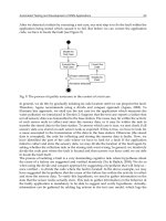
4. Firmware considerations
The microcontroller containing each autonomous probe is responsible for the smooth
running of the probe. It properly manages wireless communications, acquisition and storage
of data, and the states of work of the circuit. To achieve the requirements of energy saving,
the firmware developed for each of the autonomous probe has been structured in four
states:





Power down
Configuration
In acquisition
Down load

The “Power down” state is the key to achieving that the probes have a long life. It is the state
that stays in longer, and the state the probe enters at the end of each data collection cycle or
if it exceeds a certain amount of time without communication with the control system. To
escape the "Power down" state, a reset signal is applied to the microcontroller, which
becomes active and enters to "Configuration" mode. This mode begins a communication

with the coordinator node, where the probe is identified (ID) and receives the configuration
of the monitoring and the actual clock. After a timeout, the sensor initiates the acquisition
and the temporal buffering of temperatures, i.e., it switches to the "In acquisition" state. In